An overview of emerging pattern
mining in supervised descriptive
rule discovery: taxonomy,
empirical study, trends,
and prospects
A.M. García-Vico,
1C.J. Carmona,
2,3D. Martín,
4M. García-Borroto
4and M.J. del Jesus
1*
Emerging pattern mining is a data mining task that aims to discover discrimina-tive patterns, which can describe emerging behavior with respect to a property of interest. In recent years, the description of datasets has become an interesting
field due to the easy acquisition of knowledge by the experts. In this review, we will focus on the descriptive point of view of the task. We collect the existing approaches that have been proposed in the literature and group them together in a taxonomy in order to obtain a general vision of the task. A complete empirical study demonstrates the suitability of the approaches presented. This review also presents future trends and emerging prospects within pattern mining and the benefits of knowledge extracted from emerging patterns. © 2017 The Authors.WIREs Data Mining and Knowledge Discoverypublished by Wiley Periodicals, Inc.
How to cite this article:
WIREs Data Mining Knowl Discov2018, 8:e1231. doi: 10.1002/widm.1231
INTRODUCTION
E
merging pattern mining (EPM)1 is a data mining task that searches discriminative patterns whose support increases significantly from one class or data-set to another.Mined patterns can describe discriminative behavior between classes or emerging trends amongst datasets with respect to a property of interest by means of an understandable representation.2 In this
way, EPM is halfway between prediction and description because it describes some relationships in data, which is common in unsupervised learning tasks such as clustering, by means of a target variable typically used in classification. In fact, EPM is inter-esting for researchers in different fields like chemistry,3,4 disease detection,5,6 bioinformatics,7–9 and others10for its differentiating potential.
EPM belongs to the supervised descriptive rule discovery (SDRD) framework.2 Similar tasks in SDRD are subgroup discovery11,12 and contrast set mining.13 Thanks to its nature, EPM can be used to describe emerging or differentiating behavior with respect to a property of interest in data. Hence, the main objectives of EPM are the detection of differen-tiating characteristics between classes and the discov-ery of emerging trends in time-stamped data.1,14
This paper presents an overview of EPM from the descriptive point of view. The main objective is to demonstrate the descriptive capacity of patterns
*Correspondence to: [email protected]
1Department of Computer Science, University of Jaén, Jaén, Spain
2Department of Civil Engineering, Languages and Systems Area, University of Burgos, Burgos, Spain
3Leicester School of Pharmacy, De Montfort University, Leicester, UK
4Department of Artificial Intelligence, Technological University of La Habana, Havana, Cuba
Conflict of interest: The authors have declared no conflicts of interest for this article.
Volume 8, January/February 2018 1 of 22
extracted by emerging patterns (EPs) algorithms, according to the SDRD framework. In order to achieve this objective, the paper is organized as fol-lows: First, EPM is defined, where different kinds of EPs and the main quality measures used are described. The next section shows a taxonomy where EPs algorithms are grouped into different categories. This review is completed with a wide experimental study over a battery of datasets. The results of this work allow us to determine the suitability of different approaches presented throughout the literature and to determine new research lines in order to create new proposals focused on description. Finally, the trends and prospects of EPM are outlined.
EMERGING PATTERN MINING
The EPM problem was defined by Dong and Li1,14 as the task of finding patterns whose support increases significantly from one dataset to another.
Formally, letI= {i1,i2, …,in} be a set of
selec-tors.15 A selector is a relational statement (Attri-bute # Set), where Set is a value or a set of values that belongs to the domain of the feature Attribute, and # is a relational operator which could be =, 6¼,
2,2=, >, <,≥, ≤. A logical complex (l-complex)15 is a specific type of pattern which is a conjunction of selectors. An example E contains an l-complex, or the l-complex coversE, if Esatisfies all the selectors of the l-complex. An EP x is an l-complex whose growth rate (GR)1 is higher than a given threshold ρ≥1. This GR is defined as: the second dataset (D2). Supports are calculated as
SupD1ð Þx =
where, countDið Þx is the number of examples covered
byx in dataset i and |Di| is the number of examples
in dataseti.
The EPM was conceived from different points of view in order to describe:
• Differentiating characteristics between classes or datasets.
• Emerging trends in time-stamped datasets.
As an illustrative example, two EPs were taken from the Mushroom dataset available at the UCI reposi-tory16. This dataset contains two values for the class (edible and poisonous)1:
X=fðOdor = noneÞ, Gð :Size = broadÞ;
The results obtained for each EP are presented in Table 1. The pattern Xis an EP from Poisonous to Edible with a GR =∞, while the other EP has a GR = 21.4 from Edible to Poisonous. This means, on the one hand, that instances matching patternXonly appear in the edible class. On the other hand, instances matching pattern Y are 21.4 times more likely to appear in class poisonous than in edible. As can be observed, both patterns are simple and describe high discriminative characteristics for each class.
These patterns can be represented as rules in the form:
P:Cond!Class
where, Cond is a conjunction of selectors and Class is the value of the target variable to analyze. The pre-vious patterns could be represented as follows:
patternð ÞX : If Odor = noneð Þ ^ðG:Size = broadÞ^
TABLE 1 | Results Obtained for Different Emerging Patterns (EPs) in the Mushroom Dataset
EP SupPoisonous SupEdible GR
X 0.000 0.639 ∞
It is important to note that, by definition, patterns obtained through EPs algorithms do not satisfy the downward closure property,17 which states that sub-sets of frequent patterns are also frequent. EPM rep-resents an NP-Hard problem with respect to the number of variables18 due to the nonapplicability of such a property. Notice that the Xpattern presented in the previous example is an EP, while its sub-pattern X= {(Odor = none)}, however, is not an EP. In fact, none of its singleton sub-patterns are EPs, so the downward closure property cannot be applied anyway. The growth rate is based on the change proportion between supports and not for the current support. Therefore, a specific pattern, i.e., with high number of selectors and generally with low support, could obtain a higher change propor-tion than a general pattern, which has a lower num-ber of selectors and generally has higher support. Thus, it is not possible to achieve an exact solution in a reasonable time. However, throughout the litera-ture EPM uses the downward closure property to speed up algorithms as a pruning method, since low-support EPs are considered irrelevant.
Context of Emerging Pattern Mining
Traditionally, in data mining there are two clearly defined approaches: supervised and unsupervised learning. In general, supervised learning refers to tasks such as classification,19 regression,19 and tem-poral series analysis and classification.20 Their main aim is to predict the value of a property of interest in new incoming instances. On the other hand, unsuper-vised learning is referred to tasks such as summariza-tion21 or association rule mining.22 In this case, the aim is to describe relationships in data according to different properties such as support or confidence, and there is no interest property.
EPM attempts to build a descriptive model of data with respect to a property of interest, i.e., using supervised learning. Therefore, it is somewhere between prediction and description, because it describes some relationships between data with respect to an interest property or class. This model is built by patterns with specific characteristics in order to describe emerging or discriminative behavior in data. These descriptions should be general, simple, and as precise as possible in order to be comprehensi-ble for the experts. EPM belongs to the SDRD frame-work, which includes similar tasks such as subgroup discovery11,12 and contrast set mining.13 The main difference between EPM and subgroup discovery is that while subgroup discoveryfinds unusual distribu-tions with respect to the property of interest, EPM
finds relationships in data with respect to the possible values of the target variable. On the other hand, the difference with contrast set mining is that while con-trast set mining tries tofind patterns with high differ-ence of support, EPM tries to find patterns with a high growth rate, which allows us to describe emerg-ing tendencies in data.
Types of Emerging Patterns
EPM is considered an NP-Hard problem with respect to the number of variables. To approximate this problem efficiently, the authors have attempted to reduce the number of patterns extracted. They try to take only those patterns which describe some specific and interesting relationships between variables. This yields a more interesting and simpler set of patterns which should be as precise as possible. These types of patterns allow the description of a problem in an easy and direct way.
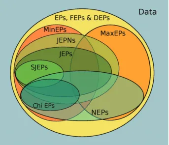
Figure 1 presents the relationships between the types of EPs most used throughout the literature, which are summarized below:
• Jumping emerging patterns(JEPs). These are EPs with a growth rate equal to infinity, i.e., the JEP covers examples for a single class. They have a great differentiator character between classes23:
JEPs =fPjGRð ÞP =∞g ð2Þ
• Minimal emerging patterns(MinEPs). A MinEP is defined as an EP whose sub-patterns are not
EPs any more. These kinds of patterns are the most general EPs. They are interesting for description because, in general, they contain a low number of variables24,25:
MinEPs =fPjGRð ÞP ≥ρ^∄SP=GRð ÞS ≥ρg ð3Þ
• Maximal emerging patterns (MaxEPs). This
type of pattern is the opposite of the minimal. A MaxEP is an EP whose super-patterns are not EPs any more. This produces very specific pat-terns, which are very precise18:
MaxEPs =fPjGRð ÞP ≥ρ^∄QP=GRð ÞQ ≥ρg ð4Þ
• Essential jumping emerging patterns (eJEPs). These are also known asstrong jumping emerging patterns(SJEPs). This type of pattern is the inter-section of the MinEPs set with the JEPs set24,25:
eJEPs =fPjGRð ÞP =∞^∄SP=GRð ÞS =∞g ð5Þ
These kinds of patterns are easy to understand and have high predictive power. They have been widely used throughout the literature due to their descriptive properties.
• Noise-Tolerant emerging patterns (NEPs). Also known asconstrained emerging patterns(CEPs). This type is very close to JEPs but it allows us to obtain precise patterns in noisy environments. Formally, a NEP fromD1toD2must satisfy25,26:
NEPs = PjSupD1ð ÞP ≤δ1^SupD2ð ÞP ≥δ2
, ð6Þ
where, normally,δ2 δ1in order to obtain patterns with a high GR.
• JEPs with negation (JEPNs). They are an exten-sion of the JEPs subset. These kinds of patterns allow the representation of negated values, i.e., a negated value represents the idea that such a value does not appear in an example. Let I denote the set of existing selectors andI=igi2I the set of selectors with negated values. The new set of possible selectors in a JEPN is defined as
P=p I [ I j 8i2ℐi2p!i2=pg. Thus, JEPNs
are defined as27:
JEPNs =fPjGRð ÞP =∞g, ð7Þ
where,P= {x1,x2, …,xn|xn2 P}. An example of
a JEPN could be the following pattern:
X=fðOdor = noneÞ, Gð :Size = broadÞ; Ring:Number = oneÞ
ð g,
which, represents those patterns without the value
nonein the variableOdor, e.g., Odor = almond, and contains (G.Size = broad) and (Ring.Number = one).
• Chi emerging patterns(Chi EPs). These are sim-ilar to NEPs but introduce aχ2statistical test in order to improve the descriptive capacity of the pattern. Chi EPs extracted are also considered as significant. A pattern is considered Chi EP when28,29:
• Sup(P)≥ξ, whereξ is the minimum support threshold.
• GR(P)≥ρ, where ρ is the minimum growth rate threshold.
• ∄SP j (Sup(S)≥ξ)^(GR(S)≥ρ)^( Strength(S)≥Strength(P)), where Strengthð ÞP =GRGRð ÞPð ÞP+ 1Sop2ð ÞP .
• jPj= 1∨jPj> 1^ 8S(SP^| S| = |P|
−1))chi(P,S)≥η, where η= 3.84 is the minimum threshold for theχ2test and chi(P,
S) is calculated through a contingency table.
Despite the efforts of researchers in extracting only those types of EPs that are relevant, most of these kinds of patterns can be extracted at once with a sin-gle execution of a mining algorithm. This is because these patterns are interrelated. Figure 1 shows the schema of these relationships. At the top level, there are classical EPs.
Inside the EPs there are some interesting groups:
• MinEPs and MaxEPs.As mentioned previously, MaxEPs are the opposite of MinEPs and they form two large groups. On the one hand, MinEPs are the most general EPs. Their proper-ties have been widely used throughout the liter-ature due to an easier mining and good results when joined with JEPs. On the other hand, MaxEPs are very specific patterns with nor-mally higher precision than MinEPs. However, mining this kind of pattern is computationally expensive.
general is the JEPNs due to the introduction of the negated values. After that, JEPs are JEPNs with only positive values. Andfinally, SJEPs are minimal JEPs, and thus are also a subset of the MinEPs. Moreover, some JEPs and JEPNs can be MaxEPs. However, the number of patterns with this condition is less than those JEPs or JEPNs that are minimal.
• The noise tolerant group. NEPs and Chi EPs
belong to this group. The NEPs is a wide set of patterns. In this set we can find some patterns that are JEPNs, JEPs, or even SJEPs. Addition-ally, the number of NEPs that can be maximal is similar to those that are minimal because more MaxEPs can fit with the conditions of NEPs. In fact, NEPs are more likely to be Max-EPs than MinMax-EPs because MaxMax-EPs tend to have higher GR due to their precision. On the other hand, Chi EPs is a subset of NEPs that tends to be minimal due to theχ2test joined with condi-tion 3.
Quality Measures
EPM has been explicitly defined with respect to the GR ((1)) measure, so it is one of the most important measures of the task.1 However, it is necessary to analyze the EPs from a new perspective. Knowledge obtained from these patterns allows the experts to learn the main discriminative characteristics between classes, or emerging trends in data, easily. In fact, this is more interesting when the amount of data grows, because it is more difficult to obtain a general and precise description of data in these environments.30 Therefore, an analysis of algorithms and patterns is necessary in order to measure characteristics that
ful-fill these requirements of knowledge. These require-ments are measured by means of the precision, generality and interest of the patterns extracted.2 This assertion is key in order to bring precise and concise knowledge to the experts.
EPs were conceived for analysis between data-sets and, for extension, between classes of a dataset. However, the number of these classes could be greater than 2, i.e., multiclass datasets. An One-vs-All (OVA)31 decomposition of the problem is neces-sary in order to deal with multiclass problems. This considers the positive class as the one represented in the consequent part of the pattern and the negative for the remaining classes, regardless of the number of classes contained in the dataset.
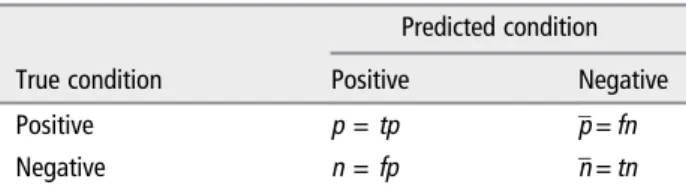
It is necessary to show the confusion matrix obtained for one pattern in order to determine its
quality.32Table 2 represents a confusion matrix for a pattern, where
• pis the number of examples correctly covered. • pis the number of examples not covered by the
class.
• n is the number of examples incorrectly covered.
• nis the number of examples not covered by the nonclass.
• p+ nis the number of examples covered by the pattern.
• p+nis the number of examples not covered by the pattern.
• Pos =p+p is the number of examples for the actual class.
• Neg =n+n is the number of examples for the remaining classes.
• T= Pos + Neg is the number of examples for the whole dataset.
For EPM, there are no measures that can esti-mate the descriptive characteristics mentioned previ-ously. However, for the SDRD framework there do exist several measures for this objective. Then, it is possible to measure the descriptive characteristics of EPs according to the SDRD framework.33A compar-ative study of the behavior of several quality mea-sures was presented in.34 In this study, the measures were classified according to their main objective and grouped following the Pearson correlation value. Fol-lowing the classification performed in this study, the most relevant measures for EPM are summarized below.
Quality Measures Based on Precision
Quality measures that belong to this group quantify the precision of a given pattern. In EPM, the acquisi-tion of patterns with high precision is important in order to obtain accurate knowledge. The most rele-vant quality measures within this group are presented below:
TABLE 2| Confusion Matrix for a Pattern
Predicted condition
True condition Positive Negative
• Growth rate (GR). This is the measure that defines an EP. It calculates the ratio between the support of the pattern in the positive class and the support in the negative. It is interpreted as the discriminative power of a pattern1:
GRð ÞP = of the predictive capacity of a pattern for the positive class, i.e., examples correctly covered among all examples covered35:
Confð ÞP = p
p+n ð9Þ
This measure can be interpreted as the accuracy of the pattern with respect to the examples it covers. It only measures precision.
Quality Measures Based on Gain Accuracy and Information
The quality measures of this group are considered as hybrids because they have different objectives: to improve the generality, precision, and interest of the pattern. The most relevant quality measures are pre-sented below:
• Weighted relative accuracy (WRAcc). Also
known as unusualness in the literature. It mea-sures the trade-off between generality and accu-racy gain36:
Where T = Pos + Neg. This value represents the bal-ance between the coverage of the pattern,p+Tnand its accuracy gain, i.e., the comparison of the accuracy obtained with respect of a naive classification by con-sidering all examples as positivepp+n−TP . It is nor-malized because the domain of this measure depends on the class analyzed.37 A high value can be inter-preted as a high balance between the generality of the pattern and its confidence.
• False positive rate(FPR). This measures the per-centage of examples incorrectly covered with
respect to the total amount of negative examples38:
FPRð ÞP = n
Neg ð11Þ
It can be interpreted as the specificity of the pattern, and normally this value must be minimized. This measure can measure both precision and generality.
• True positive rate(TPR). Measures the percent-age of examples correctly covered with respect to the total number of positive examples39:
TPRð ÞP = p
Pos ð12Þ
This can be interpreted as the sensitivity of the pat-tern. It combines precision and generality related to the class.
Quality Measures Based on Interpretability In SDRD, interpretability is defined as the ease of analysis of the results by the experts. These measures are normally related to the complete set of patterns extracted and are calculated through:
• Number of patterns (# Patterns). This measure indicates the number of patterns extracted from a given problem.
• Number of variables of the antecedent(# Vari-ables). This measure indicates to the experts the complexity of the patterns extracted. The num-ber of variables for a set of patterns is com-puted as the average of the variables for each pattern of that set.
In SDRD, a low number of patterns and variables ease the analysis.
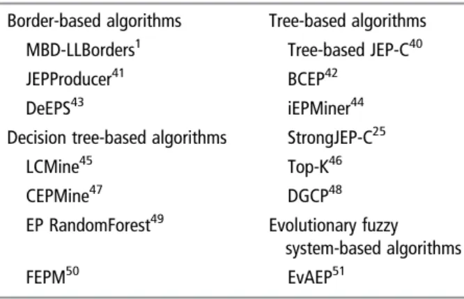
TAXONOMY FOR EPM ALGORITHMS
Border-Based Algorithms
The concept of border was introduced within thefirst definition of EPM by Dong and Li1,14as an efficient method of extraction of EPs. The border concept allows a huge number of EPs to fit into a compact representation. A border is defined as a pair hL,Ri, where L, called left-border, is a set of MinEPs and
R, called right-border, is a set of MaxEPs. This pair is considered a valid border when:
1. L andR are bothantichains. A set of patterns
S is an antichain, if 8X,Y2S,X⊈ Y
^Y⊈X.
2. Each element of L is a subset of some element of R, and each element of R is a superset of some element ofL.
These conditions allow the border to represent a con-vex space within the EP space where those patterns between Land R, i.e., thoseSsuch that XSY
where X2 L and Y2 R, are all EPs. Most of the methods within this approach use the Border-Diff procedure as their core function in order to include the borders that represent all EPs whose GR is greater than the threshold.
Figure 2 presents the general schema of border-based algorithms. First, it extracts the
borders representation of patterns that fulfill some constraints on each dataset. EPs are those patterns that are in the difference set of these borders. In order to calculate this difference efficiently, the Border-Diff procedure is executed. It handles only its borders without generating any candidate set. Within this group are the initial algorithms devel-oped for the task.
The most important algorithms in this group are:
• MBD-LLBorder.1 This is the pioneering algo-rithm for the extraction of EPs. It extracts the large borders that represent the patterns whose support is greater than a given threshold on both datasets using the Max-Miner algorithm.52 After that, it performs the Border-Diff proce-dure several times in order to obtain the differ-ence of these large borders. All patterns with a GR greater than a given threshold are returned. • JEPProducer.41This method obtains the border
representation of all JEPs. First, it obtains the horizontal border of each dataset. A horizontal border is represented as h{;}, {R1}i and it con-tains all nonzero support patterns. Then, in order to obtain JEPs it executes the Border-Diff routine to get the border which represents the difference of these sets represented by the hori-zontal borders. It also contains incremental operators in order to keep the JEPs border rep-resentation without generating the horizontal borders when new instances arrive.
• DeEPS.43 This method is based on lazy learn-ing, i.e., the training data is the model itself. For each new test instance, those selectors that do not belong to the test instance are removed from the model. After that, the JEPProducer
procedure is applied on this reduced dataset in order to obtain the border-based representation of a set of JEPs for each class that covers the test instance. The resulting set of EPs is obtained by repeating this procedure for each test instance and then removing duplicates. This TABLE 3 | Classification of the Main Algorithms for Emerging
Pattern Mining (EPM) Developed in the Literature
Border-based algorithms Tree-based algorithms MBD-LLBorders1 Tree-based JEP-C40
JEPProducer41 BCEP42
DeEPS43 iEPMiner44
Decision tree-based algorithms StrongJEP-C25
LCMine45 Top-K46
CEPMine47 DGCP48
EP RandomForest49 Evolutionary fuzzy
system-based algorithms FEPM50 EvAEP51
is currently the reference algorithm in this group for EPM.
In summary, the border-based strategy is a first approach to handle EPM efficiently. However, the complexity of the search space is exponential to the number of variables in the worst case. For this rea-son, JEPs are used in order to reduce the search space. Additionally, JEPs, which are very discrimina-tive, are very sensible to noise. The border-based rep-resentation makes the EPs obtained by this method hard to comprehend by humans. In fact, the number of patterns obtained when expanding the borders, i.e., the representation of all patterns within the bor-der, is huge if elements of L have many fewer vari-ables than those onR. So, the descriptive properties of EPs are almost useless in this representation.
Tree-Based Algorithms
The border-based strategy has an exponential com-plexity. The algorithms in this group represent the training data in a tree structure in order to efficiently mine EPs. The general mining approach that follows these algorithms is described in Figure 3.
In general, the nodes of the tree consist of a selector and the occurrence counts of the pattern formed by the path from the root to the place of the node. The root of the tree is normally a null node and the sub-tree of each child is called a component tree (CT). The selectors are sorted by a measure, which normally is GR. This keeps the most discrimi-native selectors closer to the root in order to perform a faster mining. Also, different pruning strategies can be performed in order to obtain only those EPs which are of interest. This strategy has the advantage of a faster mining than border-based methods.
However, this general scheme forces the reinsertion of instances when processing the second and consec-utive CTs in order to keep the correct counts of pat-terns.25 This normally creates a large bottleneck when mining. The most important algorithms within this group are:
• Tree-based JEP-C40 (TBJEP-C). This is thefirst method with this approach. In fact, this method can be considered as a hybrid method, because it uses the Border-Diff procedure to obtain JEPs. The aim was to improve the mining time of the JEP-Classifier algorithm53which is a clas-sification algorithm on top of JEPProducer. To achieve it, it uses a modification of the FP-Tree data structure54 to allow the use of labeled data. Each node of the tree contains the ele-ments of the general scheme presented in Figure 3 and a link to another node in the tree with the same selector. The method allows six different ordering methods for the selector when they are introduced in the tree: frequency, GR, inverse GR, hybrid, which is a weighted average between frequency and GR, least prob-able in the negative class and most probprob-able in the positive class orderings. After all examples are inserted, the mining is performed by a depth-first traversal until a node with zero counts in one class and nonzero counts in the other is found. This node is called the base node. Then, the method collects those negative instances which contain the selector in the root and the selector in the base node by means of the node-links. After that, the JEPs are extracted by implementing the Border-Diff pro-cedure using the JEP in the base node and the
negative instances collected. The experiments show a speed-up of 2 and 20 times with respect to the border-based algorithm. Moreover, it allows a minimum support-threshold pruning. • BCEP.42 This method uses the Pattern Tree
(P-Tree) structure24 to mine the complete set of SJEPs. The tree is built by sorting the selectors by GR. The mining strategy is performed by a depth-first traversal finding SJEPs. The tree is pruned by means of a minimum support thresh-old or when a JEP is found, in order to obtain only SJEPs. After that, the method keeps only the most important SJEPs with afiltering strat-egy similar to the Token Competition proce-dure.55 In this procedure, only SJEPs that can cover examples that are not already covered by better-ranked patterns are kept.
• iEPMiner44 (iEPM). This uses the P-Tree data structure to store the dataset. The objective of this algorithm is to mine Chi-EPs. The selectors are sorted by GR when building the tree. The mining procedure follows a depth-first strategy. On each node, conditions 1, 2, and 4 of Chi-EPs are checked. If the pattern fulfills these condi-tions, it is saved. The pruning strategy is based on condition 4. If the value of the χ2 test between the node and the candidate child node is less than 3.84, then the addition of the new selector does not significantly change the behav-ior of the EP, because it is independent with a 95% of confidence. In addition, the behavior of supersets that contains this selector will be the same, so the sub-tree is pruned. After finishing the tree traversal, condition 3 is checked over all patterns mined in order to obtain only Chi-EPs. • StrongJEP-C25 (SJEP-C). This algorithm mines
SJEPs with a support greater than a given threshold. To obtain these patterns, it uses a new data structure called a Contrast Pattern Tree (CP-Tree) which is similar to P-Tree, but without node-links. The algorithm builds the tree sorting the selectors by support ratio in des-cending order. This measure is defined as SuppRatioð ÞP = maxTPRFPRð Þð ÞPP TPRFPRð Þð ÞPP : The use of this measure allows patterns to be obtained for both classes in a single execution. The method mines the tree in a depth-first traversal, check-ing if the node contains zero-counts in one data-set and nonzero counts in the other, and prunes when true. In addition, it prunes when the node has a support value for both datasets lower than the threshold.
• Top-k minimal JEPs46 (Top-k). This is an
improvement of the StrongJEP method which only keeps those k patterns with the highest supports. The idea is that SJEPs with high sup-port are the most discriminative patterns. The mining scheme is similar to SJEP-C. However, the pruning strategies are different. Top-k uses two pruning strategies: first, on each node it checks if the pattern associated to the node is considered D-discernibility minimal, i.e., let
Xbe the pattern associated to the node,XisD -discernibility minimal if and only if
8YXsuppD
0
(X) < suppD0(Y), where suppD0(X) is the support of pattern for the negative class. If the node is not D-discernibility minimal, it prunes. In addition, a minimum support thresh-old pruning is used. This threshthresh-old grows dynamically by storing the patterns in a heap by nonascending support. Then if the number of elements in the heap is equal to k, the sup-port threshold is raised to the supsup-port of the
first element of the queue plus one. This allows an important pruning in the CP-Tree, obtaining the bestkpatterns much faster than SJEP-C.
• DGCP-Tree48 (DGCP). This uses a new data
structure called a Dynamically Growing Con-trast Pattern Tree (DGCP-Tree). The counts of a node are stored by the BSC-Tree structure.56 This structure allows efficient storing of the bit string which represents the examples covered by a selector. The main characteristic of this method is that the mining of EPs is performed during the construction of the tree. This mining is performed in two phases: First, the singleton selectors and BSC-Tree for both classes are identified and constructed for each one. In addi-tion, they are sorted by GR and singleton SJEPs are mined. After that, the tree grows by copying those right sibling nodes as the children of the node are being processed, if they cover new instances and their support is greater than the threshold.
fact, this approach has been widely used in the litera-ture. Nevertheless, the heuristics used by these algo-rithms for the extraction of SJEPs does not guarantee that all patterns extracted are SJEPs.
Decision Tree-Based Algorithms
Algorithms in this section induce a set of decision trees from training data. These decision trees are modified by introducing more candidate splits, where operators such as =,6¼,≤,≥, <, >,2,2= are used. The use of these operators allows the handling of numeric attributes directly without a previous discretization phase, which must be performed with border-based or tree-based approaches. Moreover, the number of EPs and their interpretability is improved by the use of these operators.
The general working schema for generating a decision tree-based algorithm is outlined in Figure 4.
The trees generated can be limited in depth in order to speed up the mining. The extraction of EPs from these trees can be performed by means of tra-versing all the paths of the tree, or performing addi-tional operations on the divided search space that produces each tree. Algorithms that follow this approach are:
• LCMine.45 This is the first algorithm that uses this approach. It generates a fixed number of trees, specified by the user. To generate a tree it is necessary to provide a vector (k1,k2, …,
kl), where l is the maximum depth of the tree
andkiis a number which indicates that thekth
best split in theith level is picked up. The infor-mation gain measure used is entropy.57 After that, a post-processingfilter is executed in order to reduce redundancy.
• CEPMine.47 This is an improvement of the
LCMine. This algorithm induces EPs from a set of C4.5 decision trees.57 The information gain
is weighted with respect to each training instance. In addition, the extraction of EPs is performed when the candidate splits are gener-ated. In this case, whenever a split contains at leastμ objects in one class and at most one in the other one, a pattern is generated even if the split is not considered the best one. After that, the best k splits are expanded, updating object weights after each induction. The tree stops when no patterns are extracted.
• EP random forest49(EP-RF). This is a modifi ca-tion of the Random Forest58 algorithm. The algorithm generates the decision trees in the same way as Random Forest. In this way, each simple decision tree creates a partitioning of the space, where instances are classified by the Ran-dom Forest algorithm. EP-RF takes the same leaf node with the same index for all generated trees. After that, examples that are within the space delimited for each tree are taken and divided into positive and negative. Once col-lected, EPs are extracted by executing the MBD-LLBorder algorithm described in this taxonomy.
• FEPM.50 This is a modification of LCMine in which the tree induction method obtains fuzzy EPs instead of crisp EPs. In this way, the calcu-lus of the information gain for each split is adapted to deal with fuzzy logic,59,60 which takes into account fuzzy memberships functions and fuzzy hedges. Also, splits are generated tak-ing into account fuzzy hedges, where each hedge is considered a potential split. A fuzzy EP (FEP) is a modification of traditional EPs which use fuzzy logic in order to represent numerical variables. The use of fuzzy logic is performed through linguistic labels, which gives an inter-pretation of numerical variables which is closer to human reasoning.61 An example of FEP is represented below:
X:fðOdor = noneÞ, Sizeð 2BroadÞ;
Ring:Number2Slightly Lowð ÞÞ
ð g, ð13Þ
where, Size 2Broad and Ring.Number 2Low are numeric variables whose values are represented by the linguistic labels Broad and Low with the fuzzy hedge Slightly, respectively. Odor = none is a cate-gorical variable.
Methods following this approach can deal with numerical attributes directly, so they evade a previ-ous discretization phase. This avoids the loss of knowledge of the problem. Moreover, the addition of operators such as inequalities, etc. or the use of fuzzy logic on numeric variables obtains patterns which are more interpretable.
Evolutionary Fuzzy System-Based
Algorithms
This type of algorithms makes use of evolutionary algorithms62 together with fuzzy logic under the name of evolutionary fuzzy systems (EFSs).63 The objective is to find very descriptive FEPs. A general schema is presented in Figure 5.
First, the algorithm initializes a population with candidates EPs through codification of the ‘ chromo-some = pattern’ approach.64 In this approach, an individual represents a potential EP. This population is evolved in order tofind high quality patterns. The evolutionary process is guided by a fitness function which measures the quality of an individual. This function could be one of the quality measures pre-sented previously or an aggregation of measures in order to find high descriptive patterns. Finally, those individuals with the highestfitness value are the EPs returned to the expert.
This group of algorithms for EPM consists nowadays of only one algorithm: EvAEP.51 This method is based on a mono-objective evolutionary algorithm.65 EvAEP follows an iterative approach where the evolutionary process is repeated until a stopping criterion is reached. The evolutionary pro-cess returns the best pattern in the population upon reaching the stopping criterion. The genetic operators used are a two-point crossover operator and a biased mutation operator.
The main advantages of this kind of method with respect to the other groups are that the search strategy performs an efficient global search through the space. Execution time can be adapted in order to
find a good balance between execution time and quality of results. The representation approaches and genetic operators can be easily adapted in order to
ease this search. In addition, it is possible to improve multiple objectives by means of multi-objective evolu-tionary algorithms (MOEAs).66,67
EXPERIMENTAL STUDY
This section outlines the results of an experimental study carried out in order to determine the quality of the patterns extracted for each method focused on descriptive induction. The behavior of a pattern with respect to this approach is determined by quality measures such as WRAcc, Conf, GR, TPR, and FPR. These measures combine several factors such as inter-pretability, precision and differentiation between sets, amongst others. Additionally, the number of patterns and the average number of variables are analyzed. In order to achieve this objective the study is structured as follows: first, the experimental framework is pre-sented, where datasets, algorithms, and statistical procedures used are shown. Then, the analyses of the results of the study are presented below.a
Experimental Setup
In this section, the experimental setup is shown. First, the characteristics of the datasets used are presented. After that, the EPs algorithms and their parameter configuration are shown. Finally, a brief explanation of the statistical tests used in the study is presented.
Datasets
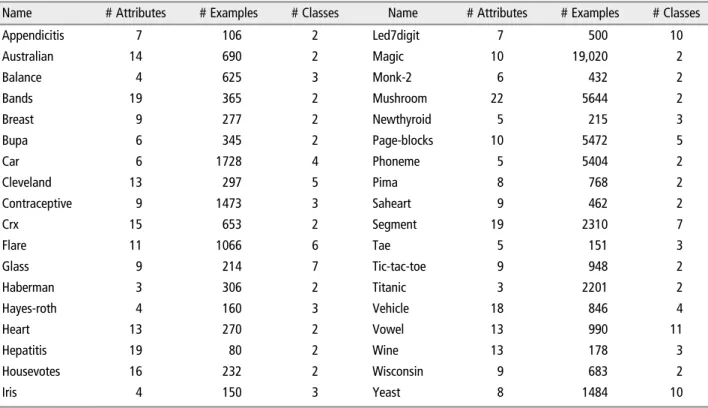
The algorithms in this study are compared with the use of 36 datasets coming from the UCI Reposi-tory.16bThis is a compilation of well-known problems which is widely used throughout the literature. Data-sets are split using a distributed optimally balanced stratified cross-validation.68 These partitions of data have been taken from the KEEL Repository.69cDetails of these datasets are summarized in Table 4, where the number of attributes together with the number of instances and classes for each one are shown.
Some algorithms work only with nominal vari-ables. Thus, a discretization of these datasets is per-formed in order to work with these methods. The discretization process used is the Fayyad discretize.70
Parameters and Base Algorithms
as possible to the other algorithms to have a fair comparison.
Due to the nondeterministic character of the EvAEP algorithm, it has been executed three times with different seeds. In this way, the results of EvAEP are the average results of the three executions on the
five partitions.
There are no public implementations of any of these algorithms. Therefore, the algorithms have been implemented following the description in the paper in which it is presented. They have been
developed in Java, and are grouped in a framework called EPM-Framework, publicly available in a website.d
Evaluation Setup
The objective of this study is determination of the descriptive capacity of the patterns extracted. In par-ticular, it is necessary to know if the descriptive knowledge obtained is as general as possible in order to be simple and interpretable. Also, the knowledge
FIGURE 5 | General schema of an evolutionary fuzzy system (EFS) algorithm for the extraction of emerging patterns (EPs).
TABLE 4| Datasets Used in the Study, Including the Number of Attributes, the Number of Examples and the Number of Classes for Each One Name # Attributes # Examples # Classes Name # Attributes # Examples # Classes
Appendicitis 7 106 2 Led7digit 7 500 10
Australian 14 690 2 Magic 10 19,020 2
Balance 4 625 3 Monk-2 6 432 2
Bands 19 365 2 Mushroom 22 5644 2
Breast 9 277 2 Newthyroid 5 215 3
Bupa 6 345 2 Page-blocks 10 5472 5
Car 6 1728 4 Phoneme 5 5404 2
Cleveland 13 297 5 Pima 8 768 2
Contraceptive 9 1473 3 Saheart 9 462 2
Crx 15 653 2 Segment 19 2310 7
Flare 11 1066 6 Tae 5 151 3
Glass 9 214 7 Tic-tac-toe 9 948 2
Haberman 3 306 2 Titanic 3 2201 2
Hayes-roth 4 160 3 Vehicle 18 846 4
Heart 13 270 2 Vowel 13 990 11
Hepatitis 19 80 2 Wine 13 178 3
Housevotes 16 232 2 Wisconsin 9 683 2
obtained should be as precise as possible. The final objective of EPM is the description of the underlying phenomena in data. For this aim, the measures stud-ied are those presented in Quality Measuressection, i.e., WRAcc, GR, Conf, TPR, FPR, number of pat-terns, and number of variables. It is important to remark that, following the results of the study pre-sented in Ref34, WRAcc, GR and Conf are not cor-related. However, TPR and FPR are highly correlated with GR. TPR is introduced to measure the generality of the patterns obtained, which is key in descriptive induction. On the other hand, FPR is introduced in order to measure the precision of pat-terns extracted, which is also a key point.
Each algorithm is evaluated over each dataset following a distributed optimally balanced stratified cross-validation68withfive folds which tries to divide the dataset into folds, keeping the data distribution as similar as possible. The advantages of using this approach are:
1. Using cross-validation allows the calculation of the quality measures over test data. Descriptive knowledge in EPM should be general because it describes the underlying phenomena of the problem. Therefore, the evaluation of EPs on test data allows us to determine whether knowledge extracted is adapted to the underly-ing phenomena.
2. Quality measures related with precision com-ponents are calculated properly.
3. The robustness of the different kinds of EPs extracted is measured because each fold slightly changes the distribution of data.
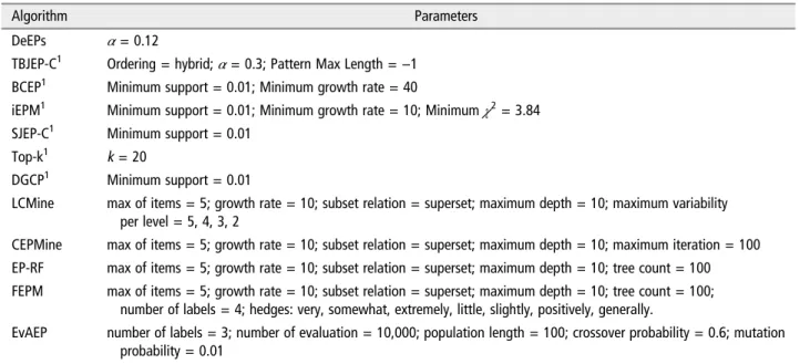
Methods are compared with a single value for quality measure and dataset. For example, ‘BCEP algorithm on WRAcc measure gets an average value of 0.6 on appendicitis dataset.’ This allows a simple compari-son between methods for each quality measure stud-ied. This value is calculated averaging, for all mined TABLE 5 | Algorithms Used and Their Parameters Configuration for the Experimental Study
Algorithm Parameters
DeEPs α= 0.12
TBJEP-C1 Ordering = hybrid;α= 0.3; Pattern Max Length =−1 BCEP1 Minimum support = 0.01; Minimum growth rate = 40
iEPM1 Minimum support = 0.01; Minimum growth rate = 10; Minimumχ2= 3.84 SJEP-C1 Minimum support = 0.01
Top-k1 k = 20
DGCP1 Minimum support = 0.01
LCMine max of items = 5; growth rate = 10; subset relation = superset; maximum depth = 10; maximum variability per level = 5, 4, 3, 2
CEPMine max of items = 5; growth rate = 10; subset relation = superset; maximum depth = 10; maximum iteration = 100 EP-RF max of items = 5; growth rate = 10; subset relation = superset; maximum depth = 10; tree count = 100 FEPM max of items = 5; growth rate = 10; subset relation = superset; maximum depth = 10; tree count = 100;
number of labels = 4; hedges: very, somewhat, extremely, little, slightly, positively, generally.
EvAEP number of labels = 3; number of evaluation = 10,000; population length = 100; crossover probability = 0.6; mutation probability = 0.01
1The method can only deal with nominal variables.
TABLE 6| Best Patterns Filters for Each Quality Measure Algorithm WRAcc Conf GR TPR FPR Selected
BCEP Conf Conf Conf Conf Conf Conf CEPMine Min Conf Min Min Conf Min DeEPS Conf Conf Conf Conf Conf Conf DGCP Min Conf Conf Min Conf Conf EP-RF Min Min Min Min – Min EvAEP – – – – – – FEPM Conf Conf – Conf Conf Conf
iEPM – – – – – –
LCMine Min Min Min Min Min Min SJEP-C Min Min Min Min Conf Min Top-K Conf Conf Conf Conf Conf Conf TBJEP-C Conf Conf Conf Min Conf Conf
patterns, the values of the quality measure using the testing datasets.
Statistical Tests for Performance
Comparison
The analysis of this study is supported by the Fried-man test.71 This test is a nonparametric statistical procedure for the comparison of more than two algo-rithms or observations. The null hypothesis is that the median of the observations are equal. The signifi -cance level considered in this study isα= 0.05. In the case of significant results, it is assumed that there are
significant differences between the algorithms. These differences can be assessed by a post-hoc method. The post-hoc method used in this experiment is the Shaffer method.72 After that, if two algorithms have significant differences the best of both is determined by the algorithm with a lower Friedman rank value. This procedure allows us to define safely the pairwise comparison of this kind of studies.
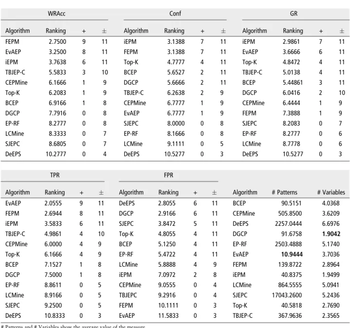
In the tables presented in this study, a highlighted result means that there are significant dif-ferences, i.e., P-value ≤α. For the comparison between algorithms or observations, like the one pre-sented in Table 7, the Friedman and Shaffer
TABLE 7| Summary of Friedman and Shaffer Test for the Different Measures Studied
WRAcc Conf GR
Algorithm Ranking + Algorithm Ranking + Algorithm Ranking +
FEPM 2.7500 9 11 iEPM 3.1388 7 11 iEPM 2.9861 7 11 EvAEP 3.2500 8 11 FEPM 3.1388 7 11 EvAEP 3.6666 6 11 iEPM 3.7638 6 11 Top-K 4.7777 4 11 Top-K 4.8472 4 11 TBJEP-C 5.5833 3 10 BCEP 5.6527 2 11 TBJEP-C 5.0138 4 11 CEPMine 6.1666 1 9 DGCP 5.6666 2 11 BCEP 5.44861 3 11 Top-K 6.2083 1 9 TBJEP-C 6.2638 2 9 DGCP 6.0416 2 10 BCEP 6.9166 1 8 CEPMine 6.7777 1 9 CEPMine 6.4444 1 9 DGCP 7.7916 0 8 EvAEP 6.7777 1 9 FEPM 7.3888 1 9 EP-RF 8.2777 0 8 SJEPC 8.0000 0 8 SJEPC 8.2083 0 7 LCMine 8.3333 0 7 EP-RF 8.1666 0 8 EP-RF 8.2777 0 6 SJEPC 8.6805 0 7 LCMine 9.1111 0 5 LCMine 8.7778 0 6 DeEPS 10.2777 0 4 DeEPS 10.5277 0 3 DeEPS 10.5277 0 3
TPR FPR
Algorithm Ranking + Algorithm Ranking + Algorithm # Patterns # Variables
EvAEP 2.0555 9 11 DeEPS 2.8055 6 11 BCEP 90.5151 4.0368 FEPM 2.6944 8 11 DGCP 2.9166 6 11 CEPMine 505.8500 3.6209 iEPM 3.5833 6 11 SJEPC 3.8472 5 11 DeEPS 2257.0444 6.6976 TBJEP-C 4.9861 4 10 Top-K 4.8055 4 11 DGCP 91.6758 1.9042 CEPMine 6.0000 4 9 BCEP 5.1250 4 11 EP-RF 2503.4888 5.1740 Top-K 6.1666 4 9 EP-RF 5.4722 4 11 EvAEP 10.9444 3.7036 BCEP 7.1527 1 8 LCMine 5.8888 4 9 FEPM 139.8722 2.8964 DGCP 7.5000 1 8 iEPM 7.0972 2 8 iEPM 40.8375 1.9499 EP-RF 8.8611 0 5 CEPMine 9.0555 0 4 LCMine 864.5555 5.0941 LCMine 8.9166 0 5 TBJEPC 9.2916 0 4 SJEPC 17043.2600 5.2436 SJEPC 9.2500 0 5 FEPM 10.1111 0 3 Top-K 40.5818 2.7690 DeEPS 10.8333 0 3 EvAEP 11.5833 0 3 TBJEP-C 367.9636 2.3565
tests,71,72 are joined and values are aggregated in order to facilitate the analysis. The table is outlined as follows: for each algorithm, the Friedman rank is obtained and methods are sorted by this value in ascending order. After that, it is necessary to deter-mine whether the differences obtained in the ranking are significant. Here two values are shown, the num-ber of algorithms is significantly better than (+) and the number of methods is equal to or better than (). ‘+’values are calculated as the number of algorithms whose P-value in the Shaffer test are lower than α and whose Friedman rankings are higher than the method analyzed. The ‘’ values are calculated as the number of algorithms whose rankings are higher than the method analyzed or whose P-values are higher than α. Therefore, one algorithm in the table is significantly better than the last ‘+’ algorithms in the table, and it is statistically equal to the nearest (‘’ - ‘+’) algorithms, beginning at the position (‘+’ +1). More information about these statistical proce-dures can be found in Ref73
The results have been obtained by means of the scmamp74package from R statistical software.75
ANALYSIS OF RESULTS
This section presents the results of the study carried out as follows:
1. The huge search space and the amount of pat-terns extracted makes EPM a problem in itself from the descriptive point of view. Thus, in order to reduce the number of patterns keeping only those with high quality, some filter gies are proposed and analyzed. These strate-gies are:
• The original set of patterns.
• The set of MinEPs. Throughout the literature, these kinds of EPs have been widely used due to their ease of mining and their discriminative power as SJEPs.
• The set of MaxEPs. This set of patterns contains the most specific patterns. It is thus interesting to show their behavior against MinEPs, which are the opposite.
• The set of EPs whose confidence is greater than 60%. Patterns with high confidence are important in order to obtain precise knowledge. Their study is interesting in order to show if precise patterns are also descriptive.
2. In the next phase, the bestfilter strategy consid-ered previously for each method is employed in
order to determine which of the proposed approaches fits better with descriptive induc-tion objectives. To do that, a comparison against all algorithms is carried out for each quality measure analyzed. This allows us to determine the best approach for each measure and give some directions in order to perform future research on those approaches that fit best with the objectives.
Filtering of Patterns
Thefirst part of the study is the selection of the best
filter strategy for each method. In order to do so, the corresponding quality measures are obtained for each
filter and algorithm. After that, Friedman and Shaffer tests are performed in order to choose the best filter on each quality measure analyzed. Once the bestfi l-ters on each measure and algorithm are determined, the best filter for an algorithm is chosen. A filter is selected if the number of quality measures where it is the best is the highest. In the case of ties, the filter with the lowest average number of patterns and vari-ables is chosen.
In conclusion, this study allows the determina-tion of the best filtering strategy and drives future research on the development of methods that can mine only these kinds of patterns, so more efficient methods with better results can be developed.
Table 6 presents a summary of the analysis per-formed, where the bestfilter for each quality measure is shown. In addition, the finalfilter chosen appears in the‘Selected’column.‘Conf’ means confidencefi l-ter and‘Min’means MinEPsfilter. The sign‘-’means the original set of patterns.
As can be observed, in the majority of algo-rithms it is necessary tofilter the complete set of pat-terns. This is due to a search strategy that finds nonrelevant EPs in some methods. Nevertheless, the iEPM and EvAEP are methods wherein these filters are not necessary due to the search strategy per-formed. Future strategies can follow a hybrid approach where the mining of minimal patterns can be performed. Nevertheless, these should be focused on those minimal patterns with the highest confi -dence in order to obtain patterns with higher descrip-tive power.
Comparison Between Algorithms
corresponding best filter applied is performed. The main objective of this part is to show which approach is most suitable for descriptive induction, which allows us to obtain a guideline for future research in thisfield. Additionally, it provides a guide of use for nonresearchers of EPs algorithms, selecting the method which bestfits its necessities.
In this websitee the complete Friedman test for
each measure is available. The tests show significant differences for each quality measure, so it is necessary to perform the post-hoc procedure in order to see which pair of methods have significant differences.
Table 7 shows the results obtained for each method regarding each quality measure. This table summarizes the results of the Friedman test and the Shafferpost-hocmethod.
The analyses of the results have been carried out for each quality measure:
• WRAcc. The algorithm with the best results in this measure is the FEPM algorithm, followed by EvAEP and iEPM. FEPM is statistically bet-ter than nine methods. EvAEP and iEPM out-perform eight and six methods, respectively. Moreover, they are better than or equal to the rest of the methods (= 11). Hence, the use of algorithms based on fuzzy logic is interesting in order to obtain patterns with high WRAcc. In addition, Chi-EPs shows a good behavior regarding this quality measure due to the use of theχ2test, which only takes those patterns that refuse the test, so they have relevant knowledge.
• Confidence. This test shows that iEPM and
FEPM obtains the best confidence results with similar ranks. They are better than seven methods. The use of Chi-EPs allows obtaining of high confidence patterns due to restriction number 3 that defines this kind of EP, which obtains patterns that cover the data very well. Additionally, the fuzzy logic used in FEPM allows a better coverage of the data, so a higher confidence value is obtained. In addition, there are three tree-based methods that are equal to or better than the rest. This result shows that the representation by a tree structure is good at the acquisition of high confidence patterns. A tree tries to find a good trade-off between the support and the specificity of the pattern, which results in high confidence patterns.
• GR.The percentage of EPs obtained in training that are also EPs on test is measured. The best results are obtained by the iEPM algorithm, which is better than seven methods, followed by
EvAEP which outperforms six. The iEPM method tends to obtain general EPs due to the support and GR restrictions that Chi-EPs have. Additionally, the patterns obtained are signifi -cant because of the χ2 test pruning method, so these kinds of patterns generalize better than other alternatives. The evolutionary strategy of the EvAEP shows a good behavior when extracting real EPs because it prefers general EPs to specific ones, these being more suitable to be EPs in a test.
• TPR.The evolutionary approach of the EvAEP algorithm obtains the best results. It is better than nine methods. It is followed by FEPM and iEPM, which outperform eight and six methods, respectively. The evolutionary strat-egy of EvAEP stimulates the production of EPs with high coverage in order to obtain a reduced set of patterns. This is interesting because it describes the data with fewest pat-terns. Fuzzy logic also plays a key role. The use of LLs is well-suited to obtaining more general patterns. In addition, the Chi-EPs is a good alternative, because of restriction number 3 which tends to obtain patterns with the highest support, so the number of examples covered is increased.
• FPR. The DeEPS and DGCP methods obtain the best results, both being better against six methods. These methods obtain patterns that are not general, as can be observed in the TPR results, but are very specific instead. This is a normal behavior of border-based methods, such as DeEPS, which are only focused on classifi ca-tion. The approach of these methods is promis-ing when patterns with a fine-grained level of description are necessary.
number of patterns is normally significantly higher with respect to the results obtained with the use of the evolutionary approach of EvAEP. • # Variables.The method with the fewest num-ber of variables on average is the DGCP method followed by the iEPM algorithm. This method’s results show that Chi-EPs and the mining strategy of iEPM are very well-suited when obtaining patterns with a low number of variables. The pruning strategy proposed on the DGCP algorithm performs very well when obtaining patterns with a low number of vari-ables. Additionally, other approaches like the use of fuzzy logic in FEPM allow us to obtain patterns with a lower number of variables.
The results of the study show that Chi-EPs used in the iEPM method obtains very good descriptive pat-terns, with high unusualness, confidence, that gener-alize very well and with good TPR values. However, the number of patterns obtained is higher than with other alternatives. The evolutionary approach of EvAEP is well-suited for description and it obtains the most reduced set of patterns, but with a high FPR value. In general, throughout the study the use of FEPs for knowledge representation is good for descriptive induction. Hence, a probably promising research line could be the hybridization of these tech-niques, e.g., fuzzy Chi-EPs with evolutionary algo-rithms as a search strategy in order to obtain descriptive patterns with high quality.
10 8 6 Interest
Int
er
est
iEPM FEPM Top–K
DGCP
BCEP TBJEP–C CEPMine EP–RF SJEPC
LCMine DeEPS
EvAEFP
4 2 0
02468
10
0 2 4
Generality
Pr
ecision
iEPM FEPM
Top–K
DGCP BCEP TBJEP–C
CEPMine EP–RF
SJEPC LCMine
DeEPS
EvAEFP
6 8 10
02468
10
0 2 4
DGCP BCEP Top–K
EP–RF LCMine
SJEPC DeEPS CEPMine
TBJEP–C EvAEFP
iEPM FEPM
6 8 10
10
86420
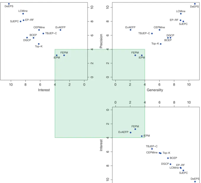
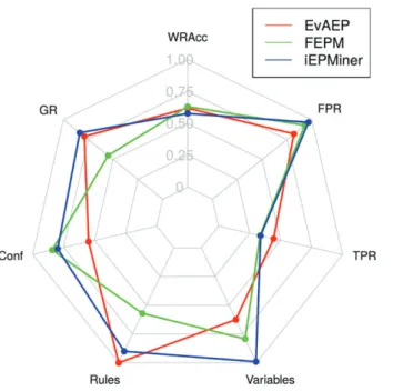
From the point of view of the SDRD frame-work, a visual summary of the most important char-acteristics of SDRD11: interest, precision and generality, measured as WRAcc, Conf, and TPR respectively, is presented in Figure 6. It shows the Friedman rank of the algorithms. The green square shows the zone with a rank lower than 4. This zone shows the most relevant and interesting approaches for future research where FEPM, iEPM, and EvAEP are within this square. Hence the approaches of these algorithms are very interesting. Additionally, a more detailed analysis of these methods is presented in Figure 7, where the behavior on all quality measures is shown. In thisfigure, GR represents the percentage of patterns extracted that are EPs on test data, Pat-terns and Variables has been normalized to appear in [0,1] and the FPR value is actually 1 FPR, in order to improve the interpretability of the chart.
On the other hand, the interpretability of results is key in order to obtain valuable knowledge. EvAEP has a much lower number of patterns than iEPM and FEPM due to the fact that EvAEP was developed to fulfill SDRD objectives, and iEPM and FEPM were developed for classification. This figure also provides a guideline for future research on the approach with better results in order to improve its behavior. As an example, the approach of EvAEP is good at TPR, so evolutionary algorithms are an interesting research line to follow in order to improve this TPR value.
Finally, the majority of the methods in the liter-ature are focused on classification and this fact is reflected in this study. Border-based methods such as DeEPS and the first tree-based algorithms such as BCEP, SJEP-C, or Top-K obtain lower values of FPR and a high number of patterns with high number of variables, which allows the obtaining of very precise patterns that are useful in classification, but are use-less for descriptive induction.
TRENDS AND PROSPECTS
In this section some relevant aspects for future research lines with the aim of obtaining more descriptive EPs methods are shown. Following the results of the complete study, possible future research areas of study are:
• Research on more evolutionary approaches for EPM. EvAEP shows good descriptive results. Nevertheless, this method is only the first one following this approach. The methodology used can be improved in many different ways, e.g., the use of MOEAs, representation based on disjunctive normal form or the use of cooperative–competitive approaches in the evo-lutionary process.
• Research on ways of efficiently mining Chi-EPs. The study reflects the high descriptive potential of Chi-EPs. Thus, the creation of new models that can efficiently mine these patterns can improve the descriptive potential of EPM in sev-eral ways.
• The introduction of fuzzy logic in EPs methods allows us to obtain high levels of unusualness and a better generality of the patterns obtained. Additionally, the knowledge obtained by these kinds of patterns is more understandable for humans.76 This fact, joined with a search strat-egy thatfinds a reduced set of patterns, allows the obtaining of valuable knowledge for experts. Thus, the use of fuzzy logic in EPM is nowadays a promising research line.
• The evolutionary approach has been demon-strated to be good in obtaining descriptive knowledge. However, there are other kinds of meta-heuristics like simulated annealing,77 swarm intelligence,78 and memetic algorithms79 amongst others that can also obtain relevant results for EPM. There is an unexploredfield of research which seems to be promising for obtaining descriptive EPs.
• Nowadays we generate high volumes of data, with great variety, at high speed in noisy envi-ronments, and it is necessary to maintain their veracity. This defines the 4V’s model of Big Data, which is a hot topic in thefields of enterprise and academia.80,81In this review, it has been shown that EPM is complex when the amount of data is huge, namely the number of variables. However, some tree-based strategies like the EP-RF algo-rithm can be easily adapted to be executed in dis-tributed environments. The descriptive point of view of EPM becomes even more important when data grow, due to it being harder to obtain a description of the data. Thus, an important research direction of EPM is on the development of methods that can deal with large amounts of data focused on description.
• This review has been focused mainly on the descriptive point of view of the task. However, it is important to remark upon the duality of EPM, where these patterns can be used as a classifier. Thus, future studies can also be focused on obtaining a good trade-off in accuracy/descrip-tion in order to exploit the full capacity of EPM. • The number of variables of the patterns extracted
for each algorithm has a direct dependent with the parameters employed in their executions. In this way, there is a need to analyze the best setup for each algorithm in order to improve the trade-off between description and interpretability. A low number of variables with good values in the different quality measures are desired.
• One of the main objectives of EPM is to find emerging trends in time-stamped data. In this way, a data stream can be considered as a spe-cial type of time-stamped data where data arrives continuously in the system in sequential order. The acquisition of knowledge from these streams can improve on-demand services like
health monitoring and trading, amongst others. However, the development of EPM for data streams is a challenge. It is necessary to adapt quality measures to this sequential data. More-over, it must be maintained incrementally in order to be efficient. The approaches presented should be adapted to data stream properties, which include infinite size, quick response, and robustness against the concept drift.82 A possi-ble first approach to deal with data streams in EPM is the use of sliding windows approaches, which allows the use of classical methods over small datasets. Nevertheless, the development of new efficient approaches is necessary with the aim of obtaining better results more efficiently.
CONCLUSIONS
This paper presents a complete study of EPM under the SDRD framework. In fact, it presents a taxonomy of the existing algorithms present in the literature and the existing kinds of EPs. Additionally, this paper presents a complete study where the Chi-EPs, and the pruning strategy based on aχ2 test are highlighted. It is impor-tant to remark that algorithms that use fuzzy logic show good values regarding the measures studied, with an easier interpretation of results. Evolutionary fuzzy sys-tems obtain good results on the measures studied. The study also highlights the importance of mining those minimal patterns with the highest confidence in order to obtain patterns with higher descriptive power.
NOTES
aDetails of this experimentation appear in the website
http://simidat.ujaen.es/papers/OverviewEPM
bhttp://archive.ics.uci.edu/ml/j chttp://www.keel.es/datasets.php
dhttp://github.com/SIMIDAT/epm-framework— ehttp://simidat.ujaen.es/papers/OverviewEPM
ACKNOWLEDGMENT
This work was partially supported by the Spanish Ministry of Economy and Competitiveness under the project TIN2015-68454-R (FEDER Founds).
REFERENCES
1. Dong GZ, Li JY. Efficient mining of emerging pat-terns: discovering trends and differences. In: Pro-ceedings of the 5th ACM SIGKDD International Conference on Knowledge Discovery and Data Min-ing, San Diego, California, USA. ACM Press; 1999, 43–52.
2. Kralj-Novak P, Lavrac N, Webb GI. Supervised descriptive rule discovery: a unifying survey of contrast set, emerging pattern and subgroup mining. J Mach Learn Res2009, 10:377–403.
mining emerging patterns from toxicity data. J Chem Inf Model2013, 5:9.
4. Lepailleur A, Poezevara G, Bureau R. Automated detec-tion of structural alerts (chemical fragments) in (eco) toxicology.Comput Struct Biotechnol J2013, 5:1–8. 5. Angriyasa PW, Rustam Z, Sadewo W. Non-invasive
intracranial pressure classification using strong jump-ing emergjump-ing patterns. In: Proceedings of the 2011 International Conference on Advanced Computer Sci-ence and Information System (ICACSIS), Jakarta, Indonesia. IEEE; 2011, 377–380.
6. Yu Y, Yan K, Zhu X, Wang G. Detecting of PIU behaviors based on discovered generators and emerg-ing patterns from computer-mediated interaction events. In: Proceedings of the 15th International Conference on Web-Age Information Management, Macau, China. Lecture Notes in Computer Science, 8485. Elsevier; 2014, 277–293.
7. Gambin T, Walczak K. A new classification method using array comparative genome hybridization data, based on the concept of limited jumping emerging pat-terns.BMC Bioinformatics2009, 10:1.
8. Piao M, Lee HG, Sohn GY, Pok G, Ryu KH. Emerging patterns based methodology for prediction of patients with myocardial ischemia. In: Proceedings of the 6th International Conference on Fuzzy Systems and Knowledge Discovery, Tianjin, China. IEEE; 2009, 174–178.
9. Tzanis G, Kavakiotis I, Vlahavas IP. Polya-iep: a data mining method for the effective prediction of polyade-nylation sites. Expert Syst Appl 2011, 38: 12398–12408.
10. Li G, Law R, Vu HQ, Rong J, Zhao XR. Identifying emerging hotel preferences using emerging pattern mining technique.Tour Manag2015, 46:311–321.
11. Carmona CJ, González P, del Jesus MJ, Herrera F. Overview on evolutionary subgroup discovery: analy-sis of the suitability and potential of the search per-formed by evolutionary algorithms.WIREs: Data Min Knowl Discov2014, 4:87–103.
12. Atzmueller M. Subgroup discovery.WIREs: Data Min Knowl Discov2015, 5:35–49.
13. Bay SD, Pazzani MJ. Detecting group differences: min-ing contrast sets. WIREs: Data Min Knowl Discov
2001, 5:213–246.
14. Dong GZ, Li JY. Mining border descriptions of emerg-ing patterns from dataset pairs. Knowledge Inform Syst2005, 8:178–202.
15. Michalski RS, Stepp R. Revealing conceptual structure in data by inductive inference.Machine Dermatol Int
1982, 10:173–196.
16. Asuncion A, Newman DJ. UCI Machine Learning Repository, 2007. Available at: http://www.ics.uci.edu/
mlearn/MLRepository.html. (Accessed August 02, 2017)
17. Agrawal R, Mannila H, Srikant R, Toivonen H, Verkamo AI. Fast discovery of association rules. In: Fayyad UM, Piatetsky-Shapiro G, Smyth P, Uthurusamy R, eds.Advances in Knowledge Discov-ery and Data Mining. Menlo Park, CA: AAAI Press; 1996, 307–328.
18. Wang Z, Fan H, Ramamohanarao K. Exploiting maxi-mal emerging patterns for classification. In:Proceedings of the 17th Australian Joint Conference on Artificial Intelligence, Cairns, Australia. Lecture Notes in Com-puter Science, 3339. Springer; 2005, 1062–1068. 19. Cherkassky V, Mulier F. Learning from Data.
Con-cepts, Theory and Methods. 2nd ed. New York: IEEE Press; 2007.
20. Box G, Jenkins G, Reinsel G. Time Series Analysis: Forecasting and Control. 4th ed. Oxford, UK: Wiley; 2008.
21. Zembowicz R, Zytkow JM. From contingency tables to various forms of knowledge in databases. In:
Advances in Knowledge Discovery and Data Mining. Menlo Park, CA: AAAI/MIT Press; 1996, 329–349. 22. Agrawal R, Imieliski T, Swami A. Mining association
rules between sets of items in large databases. In: Pro-ceedings of the 1993 ACM SIGMOD International Conference on Management of Data, Washington, D.C., USA. ACM Press; 1993, 207–216.
23. Dong GZ, Li JY, Zhang X. Discovering jumping emerging patterns and experiments on real datasets. In:Proceedings of the 9th International Database Con-ference on Heterogeneous and Internet Databases, Hong Kong. ACM Press; 1999, 155–168.
24. Fan H, Ramamohanarao K. An efficient single-scan algorithm for mining essential jumping emerging pat-terns for classification. In: Proceedings of the 6th Pacific-Asia Conference on Knowledge Discovery and Data Mining, Taipei, Taiwan. Springer; 2002, 456–462.
25. Fan H, Ramamohanarao K. Fast discovery and the generalization of strong jumping emerging patterns for building compact and accurate classifiers.IEEE Trans Knowl Data Eng2006, 18:721–737.
26. Bailey J, Manoukian T, Ramamohanarao K. A fast algorithm for computing hypergraph transversals and its application in mining emerging patterns. In: Pro-ceedings of the 3th International Conference on Data Mining, Melbourne, FL, USA. IEEE; 2003, 485–488. 27. Terlecki P, Walczak K. Jumping emerging patterns
with negation in transaction databases classification and discovery.Inform Sci2007, 177:5675–5690. 28. Fan H, Ramamohanarao K. Noise tolerant classifi
ca-tion by chi emerging patterns. In: Proceedings of the 8th Pacific-Asia Conference on Knowledge Discovery and Data Mining, Sydney, Australia. Lecture Notes in Computer Science, 3056. Springer; 2004, 201–206. 29. Ramamohanarao K, Fan H. Patterns based classifiers.