The risk-neutral stochastic volatility in interest rate models with jump-diffusion
processes
L. G´omez-Valle, J. Mart´ınez-Rodr´ıguez∗
Departamento de Econom´ıa Aplicada e IMUVA, Facultad de Ciencias Econ´omicas y Empresariales, Universidad de Valladolid, Avenida del Valle de Esgueva 6, 47011 Valladolid, Spain.
Abstract
In this paper, we consider a two-factor interest rate model with stochastic volatility and we propose that the interest rate follows a jump-diffusion process. The estimation of the market price of risk is an open question in two-factor jump-diffusion term structure models when a closed-form solution is not known. We prove some results that relate the slope of the yield curves, interest rates and volatility with the functions of the processes under the risk-neutral measure. These relations allow us to estimate all the functions with the bond prices observed in the markets. Moreover, the market prices of risk, which are unobservable, can be easily obtained. Then, we can solve the pricing problem. An application to US Treasury Bill data is illustrated and a comparison with a one-factor model is showed. Finally, the effect of the change of measure on the jump intensity and jump distribution is analyzed. JEL classification: G13, G17.
Keywords: interest rate model, zero-coupon bonds, jump-diffusion stochastic processes, stochastic volatility, risk-neutral measure, numerical differentiation, nonparametric estimation.
1. Introduction
Understanding the dynamic of the interest rates and obtaining the term structure of interest rates is important for both practical and theoretical reasons. On the one hand, it is necessary to price and hedge fixed-income derivatives and, on the other hand, it reflects market participant expectations about interest rates changes and their assessment of the monetary policy conditions. Therefore, modeling the term structure of interest rates has been the object of many studies by economists and financial institutions.
Traditionally, the financial literature assumes that interest rates move continuously and they are modelled as diffusion processes, as in [9], [32] and so on. However, more recent studies have showed that interest rates contained unexpected discontinuous changes, see for example [10] and [25]. Jumps in interest rates are, probably, due to different market phenomena such as surprises or shocks in foreign exchange markets. Moreover, when pricing and hedging financial derivatives jump diffusion models are very important, since ignoring jumps can produce hedging and pricing risk, see [26].
It is widely known that one-factor interest rate models are very attractive for practitioners because its simplicity and computational convenience. However, these models have also unrealistic properties. First, they cannot generate all the yield curve shapes and changes that we can find in the markets. Second, the changes over infinitesimal periods of any two interest-rate dependent prices will be perfectly correlated. Finally, as Hong and Li [22] show, none of their analyzed one-factor models adequately captures the interest rate dynamics. Therefore, we consider that at least two factors are necessary to model the term structure of interest rates. In fact, the number of factors must be a compromise between numerical efficient implementation and the capability of the model to fit data.
In the financial literature, for pricing financial derivatives the state variables must be considered under the risk-neutral measure because of the no-arbitrage arguments. That is, in order to obtain the derivative prices, the market is assumed to be risk-neutral and a change from the physical measure to a risk-neutral measure is necessary. However, the observations in the market are under the physical measure instead of under the risk-neutral measure, therefore the estimation can not be done directly from data in the markets. The relation between the processes under the risk-neutral and the physical measure is based on the market prices of risk. If the market prices of risk would be known, then we could easily estimate the functions of the processes under the risk-neutral measure. However, the market prices of risk are not observable either.
∗Corresponding author
In the diffusion literature, this problem is solved by considering portfolios without risk by means of no-arbitrage argu-ments, see [23] and [31] among others, but their estimation is still complex and provides small accuracy, see [15]. However, in jump-diffusion models this is not possible because the market is not complete.
Recently, in the literature, a novel approach has been considered for estimating the risk-neutral processes in one-factor models directly from data in the market, see [15] and [16] in diffusion models and [17] and [18] for jump-diffusion models. G´omez-Valle and Mart´ınez-Rodr´ıguez [18] proposed a new approach to estimate the risk-neutral interest rates in a short-rate model but, as usual in the literature, they assumed that jump size distribution did not change under the risk-neutral measure. That is, the market price of risk was assumed to be artificially absorbed by the change of measure of the jump intensity, see also [27]. Later [17] proposed a new result to estimate also the parameters of the jump size distribution directly form data in the market.
The main goal of this paper is twofold. First, we propose a new approach to estimate the whole risk-neutral functions of a two-factor model directly from data in the market. Then, we show the supremacy of this approach over a short rate model as well as the importance of assuming different functions and parameters under the risk-neutral measure to price interest rate derivatives.
The rest of the paper is organized as follows. Section 2 develops a two-factor jump-diffusion model with stochastic volatility to price interest rate derivatives. Section 3 proposes some results to estimate the whole functions of a pricing model with jumps, directly from market data, even when a closed-form solution is not known. Section 4 shows how to implement the approach in Section 3 with a nonparametric technique. Section 5 shows an empirical application to price zero-coupon bonds and bond options with data form US. Finally, Section 6 concludes. All the implementation has been done using MATLAB software.
2. The jump-diffusion model
In this section, we introduce the two-factor jump-diffusion model that we use to price interest rate derivatives. This research assumes that the state variables are the dynamics of the instantaneous interest rate,r, and the volatility,V.
Define (Ω,F,{Ft}t≥0,P) as a complete filtered probability space which satisfies the usual conditions where{Ft}t≥0 is
a filtration, see [1], [7] and [29].
In order to take into account the abrupt changes of the interest rates in the markets, we consider that the instantatenous interest rate follows a jump-diffusion stochastic process and the volatility, a diffusion process. Therefore, we consider that the factors of the model follow this joint stochastic process1:
r(t) = r(0) +
Z t
0
µr(r(z), V(z))dz+
Z t
0
V(z)dWr(z) +
Z t
0
c(r(z−), V(z))dJ(z), (1)
V(t) = V(0) +
Z t
0
µV(r(z), V(z))dz+
Z t
0
σV(r(z), V(z))dWV(z), (2)
where µrand µV are the drifts and σV the volatility of the implied volatility process. Moreover, Wr andWV are Wiener processes and the impact of the jump is given by the functioncand the compound Poisson process,J(t) =PN(t)
i=1 Yi, with
jump times (τi)i≥1, whereN(t) represents a Poisson process with intensityλ(r, V) andY1, Y2, . . .is a sequence of identically
distributed random variables with a Normal probability distribution Π,N(0, σY). We assume thatWr,WV and the jump size distribution are independent ofN, but the standard Brownian motions are correlated with
[Wr, WV](t) =ρt.
We also assume that the jump magnitude and jump arrival times are uncorrelated with the diffusion parts of the processes. Lastly, we suppose that the functionsµr, µV, σV, λ and Π satisfy suitable regularity conditions provided in the Appendix. We assume that the market is arbitrage-free. Then, there exists an equivalent martingale measure,Q-measure, which is known as the risk-neutral measure, see extended Girsanov-type measure transformation in [5] and [30]. The state variables of the model (1)-(2) under the risk-neutral measure, are as follows:
r(t) = r(0) +
Z t
0
µQr(r(z), V(z))dz+
Z t
0
V(z)dWrQ(z) +
Z t
0
c(r(z−), V(z))dJ˜Q(z), (3)
V(t) = V(0) +
Z t
0
µQV(r(z), V(z))dz+
Z t
0
σV(r(z), V(z))dWVQ(z), (4)
1ris right-continuous (cadlag, see [7]) and we denote the left limitr(t−) =lim
whereµQr =µr−V θWr,µQV =µV−σVθWV,WrQandW
Q
V are the Wiener processes underQ-measure and [WrQ, W
Q
V ](t) =ρt. The market prices of risk associated toWr andWV Wiener processes are θWr(r, V) and θWV(r, V), respectively. Finally,
˜
JQ(t) =PNQ(t)
i=1 Yi−λQtEYQ[Y1] is the compensated compound Poisson process underQ-measure and the intensity of the
Poisson processNQ(t) isλQ(r, V). Moreover, we will consider the functionc(r, V) = 1 in (1) and (3).
A zero-coupon bond price at time twith maturity timeT,t≤T, under the above assumptions, can be expressed as
P(t, r, V;T) =EQ[e−RtTr(u)du|r(t) =r, V(t) =V], (5) and at maturity it verifies thatP(T, r, V;T) = 1. Moreover, the yield curve can be obtained as
R(t, r, V;T) =−ln(P(t, r, V;T))
T−t . (6)
LetC(t, r, V, T2;T1) be the price of an European call option that matures onT1on a bond that expires atT2,T1≤T2, andK is the strike price. Then, analogously to (5), an European bond option is priced as the expected discounted payoff under theQ−measure, see [30],
C(t, r, V, T2;T1) =EQhe−RtT1r(u)du max (P(T1, r(T1), V(T1);T2)−K,0)|r(t) =r, V(t) =V
i
. (7)
Moreover,τ1=T1−tandτ2=T2−T1are the maturity of the option contract and zero-coupon bond, respectively.
3. Theoretical results
Most of the jump-diffusion models proposed for pricing interest rate derivatives are affine or linear-quadratic, see [2], [8], [9], [12], [24] and [32]. In fact, one of the main reasons is that a closed-form solution for the zero-coupon bond prices is known. However, some authors such as Duffee [11] show that affine models cannot predict accurately the expected rate of bond return.
Bandi and Nguyen [3] and Johannes [25] show how to estimate nonparametrically the functions of a jump-diffusion process by means of their moment equations for interest rate models. Though, this approach does not show how to estimate the market prices of risk. In [17] and [18] the authors propose some results to estimate the functions of the risk-neutral process in a nonparametric one-factor jump-diffusion model.
In the following result we prove several equalities which relate the slope of the yield curve and bond price with the risk-neutral drift, the volatility and the covariance of the stochastic variables.
Theorem 1. Let P(t, r, V;T)be the price of a zero-coupon bond and r andV follow the joint stochastic process given by (3)-(4), then:
∂R
∂T|T=t =
1 2 µ
Q
r +λ
QEQ
Y[Y1]
(t), (8)
∂(r2P)
∂T |T=t =
−r3+ 4r∂R
∂T|T=t+V
2+λQEQ
Y[Y
2 1]
(t), (9)
∂(r3P)
∂T |T=t =
−r4+ 2r2∂R
∂T|T=t+ 3r(V
2+λQEQ
Y[Y
2
1]) +λQEYQ[Y
3 1]
(t), (10)
∂(r4P)
∂T |T=t =
−r5+ 8r3∂R
∂T|T=t+ 6r
2(V2+λQEQ
Y[Y
2
1]) + 4rλ QEQ
Y[Y
3 1] +λ
QEQ
Y[Y
4 1]
(t), (11)
∂(V P)
∂T |T=t = µ Q
V −rV
(t), (12)
The derivatives above should be assumed as right derivatives whent∈(τi)i≥1, that is, whent is a jump time.
4. Implementation and estimation
In this section, we illustrate how practitioners can implement the results in Section 3 to estimate the functions of the risk-neutral processes in a two-factor interest rate model. Then, we propose using a nonparametric estimation technique in order to avoid imposing arbitrary restrictions on the model functions.
The term structure model we propose in Section 2 has two factors: the instantaneous interest rates and the volatility. As it is well known in the literature, the instantaneous interest rate can be proxied by different short rates in the economy, however, the volatility is not directly observable in the markets. Then, in this paper, we follow the same approach than [4] and [13], but for a jump-diffusion process. Boudoukhet al. [4] assume that the functionS(r, V), whereS is the spread between the long and short rate, is invertible. Then, implied series for the volatilityV can be estimated from the following joint stochastic process,
r(t) = r(0) +
Z t
0
αr(r(z), S(z))dz+
Z t
0
βr(r(z), S(z))dWr(z) +
Z t
0
dH(z), (13)
S(t) = S(0) +
Z t
0
αS(r(z), S(z))dz+
Z t
0
βS(r(z), S(z))dWS(z), (14)
whereαrandαS are the drifts andβr andβsthe volatilities. Moreover,WrandWS are Wiener processes and the impact of the jump is given by the compound Poisson process,H(t) = PP(t)
i=1 Xi with jump times (τ 0
i)i≥1, where P(t) represents
a Poisson process with intensity γ(r, S) and X1, X2, . . . is a sequence of identically distributed random variables with a probability distributionN(0, σX2). We assume thatWr,WS and the jump size distribution are independent of P however
dWrand dWS could be correlated.
The estimation of the implied volatility of the instantaneous interest rates can be done by means of the well-known moments of a jump-diffusion process (see for example [19] and [20])
lim
∆t↓0
1
∆tE[(r(t+ ∆t)−r(t))
2|r(t) =r, S(t) =S] =β2
r(r, S) +γ(r, S)EX[X12], (15)
lim
∆t↓0
1
∆tE[(r(t+ ∆t)−r(t))
k|r(t) =r, S(t) =S] =γ(r, S)E
X[X1k], k≥3. (16)
As we assume that the jump size follows a Normal distribution, X1 N(0, σ2
X), then, µX = EX[X1] = 0 and
σ2Y =EX[X12]. Furthermore, under this assumption of normality it is well known that
EX[X12k] =σ 2k X
k
Y
n=1
(2k−1),
EX[X12k−1] = 0, k= 1,2,3, . . .
In order to obtain the estimation of the instantaneous implied volatility series, we use (16) with k = 4 and k = 6. Finally, we obtainV(t) =βr(r(t), S(t)) using (15).
All the estimations in this paper are done using the following nonparametric approach so as to avoid imposing arbitrary restrictions in the model. Following [19] and [20], suppose a data set consists ofNobservations: (x1, y1, z1),· · ·,(xN, yN, zN), where (xi, yi) are the explanatory variables andziis the response variable. We assume a model of the kindzi=g(xi, yi)+i, whereg(x, y) is an unknown function andi is an error term, representing random errors in the observations or variability from sources not included in the (xi, yi) observations. The errorsiare assumed to be independent and identically distributed with mean zero and finite variance. The estimate has the closed-form
ˆ
g(x, y) = N
X
i=1
Wi(x, y)zi,
whereWi(x, y) is the Nadaraya-Watson product weight function:
Wi(x, y) =
Khx(x−xi)Khy(y−yi)
PN
j=1Khx(x−xj)Khy(y−yj)
, (17)
K is the Gaussian Kernel andhx andhy the bandwidths or smoothing parameters andN the number of observations, see [21]. Theoretical results for kernel regression estimators show that the optimal bandwidths will be proportional toN−1/6.
standard deviation estimates of xand y, respectively. Moreover, Φx and Φy are the scaling factors, see [4] and [13], for further details.
Once we have obtained the implied volatility series V(t) by means of nonparametric techniques, we have to estimate the different functions of the risk-neutral instantaneous interest rate and volatility stochastic processes, that is, we have to estimate the different terms in (3) and (4), but the risk-neutral variables are not observable. For this reason, the risk-neutral functions of the instantaneous interest rates and the implied volatility are estimated by means of Theorem 1 and some of the following moment equations2 of the stochastic processes (1)-(2)
Mr(r, V) = lim
∆t↓0
1
∆tE[r(t+ ∆t)−r(t)|r(t) =r, V(t) =V] =µr(r, V) +λ(r, V)EY[Y1], (18)
Mr2(r, V) = lim
∆t↓0
1
∆tE[(r(t+ ∆t)−r(t)) 2
|r(t) =r, V(t) =V] =V2+λ(r, V)EY[(Y1)2], (19)
Mrk(r, V) = lim
∆t↓0
1
∆tE[(r(t+ ∆t)−r(t))
k
|r(t) =r, V(t) =V] =λ(r, V)EY[(Y1)k], k≥3, (20)
MV(r, V) = lim
∆t↓0
1
∆tE[(V(t+ ∆t)−V(t))|r(t) =r, V(t) =V] =µV(r, V), (21)
MV2(r, V) = lim
∆t↓0
1
∆tE[(V(t+ ∆t)−V(t)) 2
|r(t) =r, V(t) =V] =σV2(r, V). (22)
Each of the derivatives from (8) to (12) are approximated using numerical differentiation. More precisely, we apply a second order forward difference formula to obtain greater accuracy, see [6].
Firstly, we estimate the risk-neutral interest rate drift by means of (8). We approximate the partial derivative ∂R∂T|T=t as follows
∂R(t, T)
∂T |T=t=
−3R(t, t) + 4R(t, t+ ∆)−R(t, t+ 2∆)
2∆ +O(∆
2), (23)
with a step size ∆>0. Then, we apply the Nadaraya-Watson estimator (17) to obtain its nonparametric estimation.
Secondly, we approximate ∂(∂Tr2P)|T=t and ∂(r4P)
∂T |T=t with a similar second order approximation to (23), interest rate and price data and we replace them in (9) and (11). Then, as EQ[Y2] = σ2
Y and EQ[Y2] = 3σ4Y, we estimate σ2Y by means of the relation between (9) and (11) and the Nadaraya-Watson estimator. Next, we replace this estimation in (9) to estimate nonparametrically the jump intensity underQ-measure, λQ.
Thirdly, we estimate the risk-neutral drift of the volatility. We approximate numerically ∂(∂TV P)|T=t with a similar second-order approximation to (23), we replace it in (12) and we estimateµQV by means of the Nadaraya-Watson estimator. As far as the σV is concerned, this function do not change under Q-measure. Therefore, for its estimation we use the second-order moment of a diffusion process (22) and the Nadaraya-Watson estimator in (17), see [4] among others.
Finally, for pricing zero-coupon bonds or any other interest rate derivative, we need the covariance of the two state variables of the model. From the moment equation,
Mr,V(r, V) = lim
∆t↓0
1
∆tE[(r(t+ ∆t)−r(t))(V(t+ ∆t)−V(t))|r(t) =r, V(t) =V] =ρ(r, V)V σV(r, V),
and the Nadaraya-Watson estimator, we estimate this covariance, see [4], [19] and [20].
In the literature, the estimation of all the functions under the risk-neutral measure is usually quite complex and time-consuming. Therefore, for simplicity some assumptions are made. Sometimes the market prices of risk are assumed to be zero for the diffusion part or one for the jump part of the processes. This means that the functions of the stochastic processes and the jump size distribution parameters are equal under the physical and the risk-neutral measure. In order to analyse the effect of the change of measure on the yield curves, we consider the following assumptions:
(i) Assumption A1 (P-Total). We assume that the instantaneous interest rates and the implied volatility processes are equal under the P and the Q-measure. This means that λQ(r, V) = λ(r, V), θWr = 0, θWV = 0 and that the jump distribution do not change. In this case, all the estimations are done with the moment equations (18)-(22) and the Nadaraya-Watson estimator. Theorem 1 is not taken into account.
(ii)Assumption A2(R-NJI).We assume that the jump size distribution underQ-measure of the jump-diffusion process is equal to the distribution underP-measure. This means that all risk premia related to the jump distribution are artificially
absorbed by the change in the intensity of the jump fromλunder the physical measure toλQunder the risk-neutral measure, see [27]. Then,
EYQ[Y1] = EY[Y1] = 0,
EYQ[Y12] = EY[Y12] =σ 2
Y.
So as to estimate this model, we use the results of Theorem 1 and the moment equations as follows. We estimate the volatility of the implied volatility and the parameters of the jump size distribution with the moment conditions (19), (20) and (22) and the Nadaraya-Watson estimator. Then, the rest of the risk-neutral functions are estimated using (8), (9) and (12) in Theorem 1, numerical approximation (23) and Nadaraya Watson estimator.
(iii)Assumption A3 (R-NJS).We assume that the jump intensity underQ-measure is equal to the jump intensity under P-measure. This is equivalent to assume thatλQ(r, V) = λ(r, V) and it means that all risk premia related to the jump intensity are artificially absorbed by the change in the parameters of the jump size distribution. In this case, we estimate the intensity of the jump process and the volatility of the implied volatility with the moment conditions (19), (20) and (22) and the Nadaraya-Watson estimator. Then, the rest of the risk-neutral functions are estimated using (8), (9) and (12) in Theorem 1, numerical approximation (23) and Nadaraya-Watson estimator. Notice that (11) in Theorem 1 is not used to estimate the functions of the model under the assumptionsA2 andA3.
(iv) Assumption A4 (R-NTotal). We assume that all the functions are different under P-measure and Q-measure. Therefore, all functions are estimated using Theorem 1 apart fromσV(r, V), which is estimated using the moment equation (22), as previously described in detail.
5. Empirical analysis
In this section, we apply the results in Section 2 to recent U.S. Federal Reserve interest rate data (Federal Reserve h.15 database) to obtain the yield curves. Then, we show that considering two state variables in an interest rate model, more precisely considering the volatility as well as the instantaneous interest rates as state variables, improve considerably the yield curves. Finally, we analyze the role of the different market prices of risk implicitly considered for obtaining the yield curves and pricing bond options.
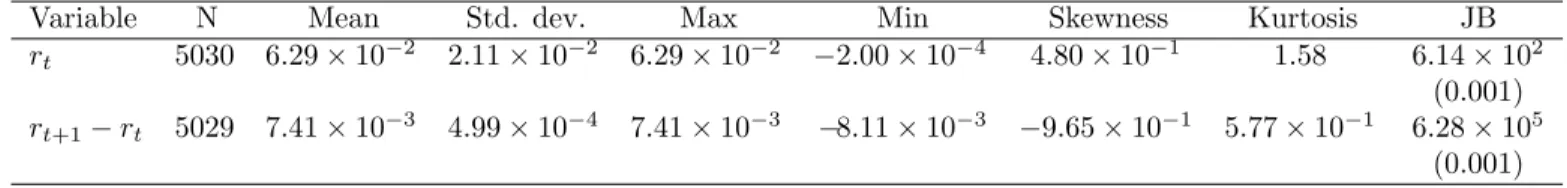
The instantaneous interest rates are not observable in the markets. Then, as usual in the literature (see [15], [18], [25], etc.), we use the daily 3-month T-Bill rates as proxy of this rate. Figure 1 depicts the time series of the daily 3-month T-Bill rates and their daily changes from January 1997 to February 2017. This figure shows the behaviour of the in-sample data (January 1997-December 2016) and the out-of-sample data (January-February 2017).
Table 1, reports the main descriptive statistics of the data. Both skewness and kurtosis statistics indicate that interest rates are not Normally distributed, which is further confirmed by results of the Jarque-Bera test (JB) for normality in the last column (p-values on brackets). In fact, this series exhibits significant excess kurtosis meaning that as compared to a Normal distribution, it has higher and sharper central peak and longer fatter tails. Hence, a jump-diffusion process is more suitable for modelling the interest rates.
Variable N Mean Std. dev. Max Min Skewness Kurtosis JB
rt 5030 6.29×10⁻² 2.11×10⁻² 6.29×10⁻² −2.00×10⁻⁴ 4.80×10⁻¹ 1.58 6.14×10² (0.001)
rt+1−rt 5029 7.41×10⁻³ 4.99×10⁻⁴ 7.41×10⁻³ −8.11×10⁻³ −9.65×10⁻¹ 5.77×10⁻¹ 6.28×10⁵ (0.001)
Table 1: Summary of the statistics on the 3-month T-Bill rates and the first differences, January 1997-February 2017.
As far as the implied volatility is concerned, we use the approach in Section 4 for its estimation. As the implied volatility is not observable, we use the difference between the yields on US Treasury Securities at constant 10-year maturity and the 3-month T-Bill rates as a proxy forS(t), following [4] and [13]. Then, we obtained the implied volatility series by means of nonparametric techniques as in Section 4.
Firstly, with these data (January 1997-December 2016) and following the implementation and estimation approach in Section 4, we estimate all the risk-neutral functions. Then, we price zero-coupon bonds by means of the conditional expectation in (5). As we have considered a nonparametric approach to estimate the whole functions of the risk-neutral stochastic processes3, a closed-form solution for this model cannot be obtained. Hence, a numerical method is necessary
3All the scaling factors in the bandwidths(h
Time
97 98 99 00 01 02 03 04 05 06 07 08 09 10 11 12 13 14 15 16 17
Interest rates
0 0.02 0.04 0.06
Time
97 98 99 00 01 02 03 04 05 06 07 08 09 10 11 12 13 14 15 16 17 Differences in interest rates -0.01
-0.005 0 0.005 0.01
Figure 1: 3-month Treasury Bill rates and their first differences, January 1997-February 2017.
to price zero-coupon bonds. More precisely, we use the Monte Carlo simulation approach with 5000 simulations and a daily time step (1/250). This method is widely used in the literature and by practitioners in the markets, especially for multi-factor models, because of its simplicity and efficiency, see [14]. Next, we obtain the yield curves with (6).
In order to show the supremacy of this two-factor model over a one-factor model, we also obtain the yield curves with a short-rate model with a risk-neutral jump-diffusion instantaneous interest rate process as follows:
r(t) = r(0) +
Z t
0
µQr(r(z))dz+
Z t
0
σr(r(z))dWrQ(z) +
Z t
0
dJ˜Q(z), (24)
where µQr =µr−σrθWr and WrQ is the Wiener process under Q-measure andθWr is the market price of risk associated to the Wiener processes. Finally, ˜JQ(t) = PNQ(t)
i=1 Yi−λQtEY[Y1] is the compensated compound Poisson process under Q-measure,λQ(r) is the intensity of the Poisson processNQ(t) andY1, Y2, . . .is a sequence of identically distributed random variables with Normal distribution.
Recently, [18] proposed a novel approach to estimate this one-factor interest rate model directly from market data and they also use nonparametric methods and Monte Carlo simulation approach to obtain the yield curves. Then, we will use this approach to obtain the yield curves in the out-of-sample.
In this section, so as to make comparisons, we use the root mean square error (RMSE) and the percentage root mean square error (PRMSE) for the out-of-sample (January-February 2017):
RM SE =
v u u t
1
n
n
X
t=1
Rt−Rˆt
2
,
P RM SE =
v u u t1
n
n
X
t=1
Rt−Rˆt
Rt
!2
,
in Table 2, when we consider the previous one-factor jump diffusion model (1Var) the RMSE is considerably higher than when we consider our two-factor model in Section 2 when all the risk-neutral functions are estimated directly from data in the market using Theorem 1. The difference between the percentage errors are also very important, they are nearly 20%.
1Var PMTotal R-NJS R-NJI R-NTotal
RMSE 3.3675×10⁻³ 1.0742×10⁻³ 8.2942×10⁻⁴ 7.5629×10⁻⁴ 7.5064×10⁻⁴
PRMSE 23.8% 8.8% 6.2% 5.5% 5.5%
Table 2: RMSE and PRMSE for the out-of-sample, January-February 2017.
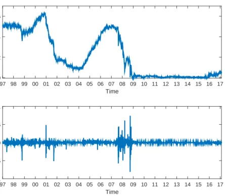
For a more in-depth analysis of the behaviour of the 1Var and R-NTotal models, we plot in Figure 2 the yields to maturity for a short maturity (6 months) and a long maturity (5 years) along the whole out-of-sample. As we can see, in general, the 6 month yields to maturity with both models undervalue the yields to maturity. However, the R-NTotal yields are always slightly closer to the observed yields than the 1Var yields. In the bottom part of Figure 2, we plot the yields to maturity for a high maturity (5 years) with both models. We see that the yields obtained with the R-NTotal model are much closer to the observed yields to maturity. Furthermore, meanwhile the R-NTotal yields overvalues the real yields to maturity, the 1Var yields undervalues then considerably.
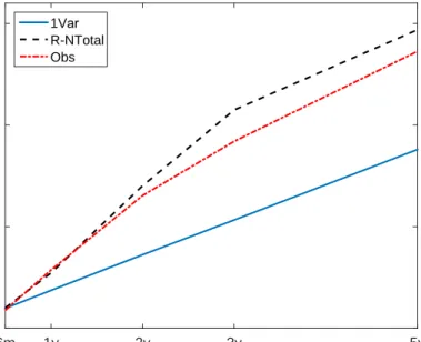
In Figure 3, we plot the observed yield curve and those estimated with 1Var and R-NTotal models on January, 2 2017. We see that both models predict a positively sloped yield curve and that the R-NTotal model fits the observed term structure relatively well unless for maturities till two years. However the 1Var model underestimates considerably the yield curve for all maturities. We have also analyse the yield curves on other different days of the out-of-sample period, but the supremacy of the R-NTotal model over the 1Var model does not change. These facts are very interesting because the term structure of interest rates is an important instrument for analyzing the economy. Therefore, a good prediction of this instrument can help investors and politicians.
It is very well-known that interest-rate derivative prices are obtained as conditional expectations under the risk-neutral measure (see for example (5) and (7)) because of non-arbitrage arguments. This fact gives as a result that some new functions are added to the models: the market prices of risk. These functions are unobservable and, therefore, very difficult to estimate. In consequence, in order to simplify, some assumptions are usually considered in the literature, as we have previously stated in Section 4. In this section, we also analyse the effect of these assumptions over the yield curves.
In Table 2, we show the RMSE and PRMSE of the different assumptions about the market prices of risk. When we consider that all the functions are equal under the physical and the risk-neutral measure (P-Total) we have the highest RMSE in the two-factor models, apart from the 1Var model. Then, assuming that the risk-neutral intensity of the jump is equal to the intensity of the jump under the physical measure (R-NJS) provides lower RMSE. Moreover, if the risk-neutral jump size distribution is equal under both measures (R-NJI), then the RMSE decreases. Finally, if we assume that all the functions are different under the physical measure and the risk-neutral measure (R-NTotal) we get the lowest RMSE. As far as the PRMSE is concerned, we get the same conclusions although the R-NJI and the R-NTotal provide the same PRMSE. Therefore, it is worthwhile to estimate correctly all the risk-neutral functions although sometimes it is a complex and difficult task. Nevertheless, assuming that the jump size distribution under Q-measure is equal than the jump size distribution provides nearly similar errors than the R-NTotal model.
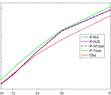
So as to compare the yield curves provided by the previous assumptions, we plot then in Figure 4. All the estimated yield curves are positively slope curves as the observed yield curve but there are differences between them. Assuming that all the functions under theQ-measure are equal to those under the physical measure (P-Total), the estimated yield curve overvalues considerably the real yield curve. However, when we assume that some or all the functions of the stochastic processes are different under the physical and Q-measure and Theorem 1 is used for its estimation the results improve considerably, especially for maturities till 2 years. However, in this plot we can not discern the advantages or disadvantages of considering the R-NTotal, R-NJS or R-NJI models. The yield curves on this figure are on 2 January 2017. We have also considered the yield curves on other different days and the conclusions are quite similar and the differences too small to distinguish among the previous models.
Time
1 Jan 17 20 Jan 17 5 Feb 17
Yield to maturity
#10-3
5.6 5.8 6 6.2 6.4 6.6 6.8
6 months
Time
1 Jan 17 20 Jan 17 5 Feb 17
Yield to maturity
0.014 0.016 0.018 0.02
5 years
1Var R-NTotal Obs
Figure 2: The yields to maturity for the out-of-sample (January-February 2017) for maturities: 6 months and 5 years. The blue solid line is the 1Var yield curve, the black dashed line is the R-NTotal yield curve and the red dash-dot line is the observed yield curve.
Maturity
6m 1y 2y 3y 5y
Yield to maturity
0.005 0.01 0.015
0.02 1Var
R-NTotal Obs
overestimate the yields to maturities and the R-NTotal and R-NJI are the closest to the observed yield curves. Although the differences between these two models are not very important, the R-NTotal is the closest to the observe yields in most of the cases. This fact is consistent with the values of the RMSE and PRMSE showed in Table 2.
Therefore, we can conclude that a two-factor models is more accurate to obtain the yield curves than a one-factor model. Moreover, once we consider a two-factor model, it is very important to take into account an accurate estimation of the whole risk-neutral functions. Although assuming that the jump size distribution under Q-measure is equal to the distribution underP-measure can provide quite accurate results. This fact is consistent with the results in [17] for one-factor models.
The errors in estimating the yield curves are usually magnified when pricing other interest rate derivatives. Then, in this section, we also analyze the differences between the option prices with the R-NTotal model and those assumptions which provide better yield curves: R-NJI and R-NJS. In order to make comparisons, we price options with different maturities (τ1 = 3,6 and 12 months), and different underlying zero-coupon bond maturities (τ2 = 3,6 and 12 months) on 2 January
2017. These option prices are obtained by means of (7) and the Monte Carlo simulation approach. We use the same in-sample data that for the yield curves and run 5000 simulations with a daily time step (1/250).
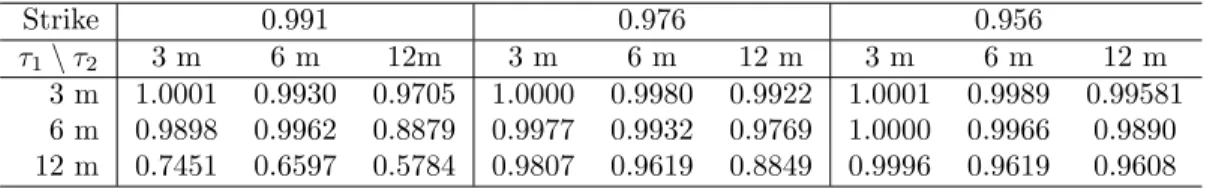
Strike 0.991 0.976 0.956
τ1\τ2 3 m 6 m 12m 3 m 6 m 12 m 3 m 6 m 12 m
3 m 1.0004 0.9991 1.0009 1.0001 0.9997 1.0003 1.0001 0.9999 1.0001 6 m 0.9997 0.9959 1.0041 0.9999 0.9992 1.0003 1.0000 0.9996 1.0001 12 m 0.9830 0.9670 0.9862 0.9991 0.9970 1.0001 0.9996 0.9989 1.0000
Table 3: Ratios between the R-NTotal and R-NJI option prices (R-NTotal price/R-NJI price).
Strike 0.991 0.976 0.956
τ1\τ2 3 m 6 m 12m 3 m 6 m 12 m 3 m 6 m 12 m 3 m 1.0001 0.9930 0.9705 1.0000 0.9980 0.9922 1.0001 0.9989 0.99581 6 m 0.9898 0.9962 0.8879 0.9977 0.9932 0.9769 1.0000 0.9966 0.9890 12 m 0.7451 0.6597 0.5784 0.9807 0.9619 0.8849 0.9996 0.9619 0.9608
Table 4: Ratios between the R-NTotal and R-NJS option prices (R-NTotal price/R-NJS price).
Table 3 shows the ratios between the R-NTotal option prices and the R-NJI option prices. As we can see, the differences between these ratios are very small. Therefore, they could be considered nearly negligible, although the differences are slightly higher than when the yield curves are obtained.
The ratios between the R-NTotal option prices and the R-NJS option prices are showed in Table 4. In this case, nearly all the zero-coupon bond option prices with our approach are lower than with the assumption R-NJS. However, the differences are higher for some maturities and exercise prices than those in Table 3.
Therefore, it is very interesting to consider a correct risk-neutral estimation of all the functions of a model, but assuming that the all risk premia related to the jump distribution are artificially absorbed by the change of the jump intensity could be quite acceptable for not very high maturities, because the differences are not very important.
6. Conclusions
In order to avoid arbitrage opportunities in a term structure model, a change of measure from the physical measure to the risk-neutral measure is necessary. This fact introduces some new functions in the model which are called market prices of risk. These functions are unobservable and very difficult and complex to estimate. In fact, in two-factor jump-diffusion models, this issue is still an open-question.
In this paper, we assume a two-factor jump diffusion model where the state variables are the instantaneous interest rate and the volatility. This model takes into account the possible abrupt changes of the interest rates in the markets. Then, we prove several equalities which relate the slope of the yield curves with the functions of the risk-neutral stochastic processes and the state variables. The main point of this result is that it allows estimating the whole risk-neutral functions directly from data in the markets, even when a close form-solution for the pricing model is not known.
Maturity
6m 1y 2y 3y 5y
Yield to maturity
0.005 0.01 0.015 0.02
R-NJI R-NJS R-NTotal P-Total Obs
Figure 4: Yield curves on 2 January 2017. The blue dotted line is the R-NJI yield curve, the magenta solid line is the R-NJS, the black dashed line is the R-NTotal yield curve, the green solid line is the P-Total and the red dash-dot line is the observed yield curve.
Time
1 Jan 17 20 Jan 17 5 Feb 17
Yield to maturity
#10-3
5.6 5.8 6 6.2 6.4 6.6 6.8
6 months
Time
1 Jan 17 20 Jan 17 5 Feb 17
Yield to maturity
0.018 0.019 0.02
0.021 5 years
R-NJI R-NJS R-NTotal P-Total Obs
the functions are estimated directly from market data and numerical methods are applied to obtain accurate approximated solutions.
In order to show the supremacy of this two-factor model and the approach we propose, we make two comparisons. First, we compare this two-factor model with a one-factor model where the risk-neutral functions are estimated nonparametrically and directly from market data as in [18], where the effect of the change of measure in the jump size distribution is not taken into account. In this case we obtain that the two-factor model provides much more accurate yield curves than the one-factor model.
Finally, so as to analyze the importance of estimating the whole risk-neutral functions accurately, we make some different assumptions. If we assume that the jump distribution under the risk-neutral measure is equal to the distribution under the physical measure, we obtain quite accurate results: the RMSE is slightly higher than when all the functions are assumed under the risk-neutral measure. However, if we assumed that the jump intensity is equal under the physical and the risk-neutral measure the errors increase.
Therefore, considering a term structure model with two factors (the instantaneous interest rate and the volatility) provides more accurate yield curves than a one-factor model. Moreover, a precise estimation of all the risk-neutral functions is also very important, although assuming that the jump size distribution is equal under both measures, as usual in the literature, provides low differences which in some cases could be even nearly negligible. These conclusions are also valid for other interest rate derivatives such as zero-coupon bond options.
Acknowledgements
The authors are grateful to the anonymous referees for their constructive suggestions and helpful comments. This work has been supported in part by the project MTM2017-85476-C2-P of the Spanish Ministerio de Ciencia, Innovaci´on y Universidades. Also by the projects VA041P17 of the Junta de Castilla y Le´on and European FEDER Funds and VA148G18 of the Junta de Castilla y Le´on.
Appendix
This appendix states the regularity conditions that guarantee the existence and uniqueness of the stochastic differential equations considered in this paper. These conditions are necessary to prove Theorem 1.
In the following assumptions, we consider the notation form of the functions in (1)-(2): µ= (µr, µV) andσ= (V, σV).
• Assumption 1 The functionsµ, σ andλ are twice continuously differentiable and we consider that c(r, V) = 1 in (2) along this paper. Moreover, they satisfy local Lipschitz and growth conditions. That is, for every compact subset
D⊂R2, there exists a constantC1Dsuch that, for allx, z∈D,
|µ(x)−µ(z)|+|σ(x)−σ(z)| ≤C1D|x−z|.
• Assumption 2There exists a constantC2 such that for anyx∈R2,
|µ(x)|+|σ(x)|+λ(x)
Z
R
|y|Π(dy)≤C2(1 +|x|).
• Assumption 3For anyα >2, there exist a constantC3 such that for anyx∈R2
λ(x)
Z
R
|y|αΠ(dy)≤C3(1 +|x|α).
• Assumption 4λ(x)≥0 andσ2(x)>0 on
R2.
The above conditions on the model guarantee the existence and uniqueness of a cadlag strong solution to (1)-(2), see [28], [3]. Similar conditions must be verified by the functions of the stochastic processes (13)-(14) and (24).
Then, we prove the Theorem 1 in Section 3.
Proof of Theorem 1.
LetD(t) = e−R0tr(s)ds denote the discount process and then
Therefore, we obtain:
D(T+h)−D(T) =
Z T+h
T
−r(z)D(z)dz.
We calculate the conditional expectation underQ-measure in the above equality and taking into account (5), we get
P(t, r, V;T +h)−P(t, r, V;T) =EQ
" Z T+h
T
−rDdz|r(t) =r, V(t) =V
#
.
Now dividing byhand taking limits, whenhtends to 04, we have
∂P
∂T(t, r, V;T) =−r(t)P(t, r, V;T). (26)
Using Itˆo’s product rule, see [30] and [7], and the equalities (25) and the differential form of interest rate stochastic process (3), we have
d(rD) =D(−r2+µQr +λQEQ[Y1])dt+DV dWrQ+
d
NQ(t)
X
i=1
D(τi−)Yi
−D(t−)λQEQ[Y1]dt
. (27)
We consider the integral form of (27)
r(T+h)D(T+h)−r(T)D(T) =
Z T+h
T
D(z)(−r2+µQr +λQEQ[Y1])(z)dz+
Z T+h
T
DV dWrQ(z)
+
NQ(T+h)
X
i=NQ(T)+1
D(τi−)Yi
−
Z T+h
T
D(z−)λQEQ[Y1]dz
,
and we calculate the conditional expectation under Q-measure. Taking into account (5) and the fact that the Itˆo integral and compensated process are martingales, the conditional expectation underQ-measure of the last terms is zero. Then, we obtain
r(T+h)P(t, r, V;T+h)−r(T)P(t, r, V;T) =
Z T+h
T
P(t, r, V;z) −r2+µQr +λQEQ[Y1]
(z)dz,
and dividing byhand taking limits, whenhtends to 0,h↓0, then
∂(rP)
∂T (t, r, V;T) =P(t, r, V;T) −r 2
+µQr +λQEQ[Y1]
(T). (28)
Due to (26), we have ∂(∂TrP)(t, r, V;T) = −∂2P
∂T2(t, r, V;T), and using (6) and (28), we obtain (8). Using Itˆo’s product rule and (27) we have
d(r2D) = D(−r3+ 2rµQr +V2+ 2rλQEQ[Y1] +λQEQ[Y12])dt
+ 2rDV dWrQ+
d
NQ(t)
X
i=1
D(τi−)(2r(τi−)Yi+Yi2)
−D(t−)λ
Q(2r(t−)EQ[Y1] +EQ[Y2 1])dt
. (29)
With the integral form of (29) and using the same steps as above, we get (9) Now, as earlier, using Itˆo’s product rule and (29) and (3) we have
d(r3D) =D −r4+ 3r2(µQr +λQEQ[Y1]) + 3rV2+ 3rλQEQ[Y12] +λQEQ[Y13]dt+ 3r2DV dWrQ
+
d
NQ(t)
X
i=1
D(τi−)(3r2(τi−)Yi+ 3r(τi−)Yi2+Y
3
i )
−D(t−)(3r
2(t−)EQ[Y1] + 3r(t−)EQ[Y2 1] +E
Q[Y3 1])dt
.(30)
Using the similar reasoning above, we obtain (10). Using Itˆo’s product rule and (30) and (3) we have
d(r4D) = D −r5+ 4r3(µQr +λQEQ[Y1]) + 6r2(V2+λQEQ[Y12]) + 4rλQEQ[Y13] +λQEQ[Y14]
dt
+ r2D(3 +V)dWrQ+d
NQ(t)
X
i=1
D(τi−)(3r3(τi−)Yi+ 6r2(τi−)Yi2+ 4r(τi)Yi3+Y
4
i )
− D(t−)λQ(3r3(t−)EQ[Y1] + 6r2(t−)EQ[Y12] + 4r(t−)EQ[Y 3
1] +EQ[Y 4 1])dt.
In the same way, using similar reasoning above, we obtain (11).
Using the Itˆo’s product rule, (25) an the integral form of (4), we have
d(V D) =D(−rV +σVQ)dt+DσVdWVQ. (31) We consider the integral form of (31)
V(T +h)D(T+h)−V(T)D(T) =
Z T+h
T
D(z)(−rV +σVQ)(z)dz+
Z T+h
T
DσVdWVQ(z)
and we calculate the conditional expectation underQ-measure. We divide byhand take limits, whenhtends to 0, then,
∂(V P)
∂T (t, r, V;T) =P(t, r, V;T)(−rV +µ Q
V)(T),
and we get (12).
Bibliography
[1] D. Applebaum, L´evy Processes and Stochastic Calculus. Cambridge University Press, Cambridge, 2009.
[2] T.G. Andersen, L. Benzoni, J. Lund, Stochastic volatility, mean drift, and jumps in the short-term interest rate. Working Paper, Northwesterm University, University of Minnesota and Nykredit Bank, 2004.
[3] F.M. Bandi, T.H. Nguyen, On the functional estimation of jump-diffusion models, J. Econometrics 116 (2003) 293-328.
[4] J. Boudoukh, C. Downing, M. Richardson, R. Stanton, A multifactor, nonlinear, continuous-time model of interest rate volatility. In: Tim Bollerslev, Jeffrey R. Russell, and Mark W. Watson (eds.), Volatility and Time Series Econometrics. Essays in Honor of Robert F. Engle. Oxford University Press, New York, 2010.
[5] P. Bremaud, Point Processes and Queues. Martingale Dynamics. Springer-Verlag New York, New York, 1981.
[6] R.L. Burden, J.L. Faires, Numerical Analysis. Brooks/Cole Publishing Co, New York, 2001.
[7] R. Cont, P. Tankov, Financial Modeling with Jump Processes. Chapman and Hall/CRC, Boca Raton, Florida, 2004.
[8] T. Corzo Santamaria, J. G´omez Biscarri, Nonparametric estimation of convergence of interest rates: Effects on bond pricing, Span. Econ. Rev. 7 (2005) 167-190.
[9] J.C. Cox, J.E. Ingersoll, S.A. Ross, A theory of the term structure of interest rates. Econometrica 53 (1985) 385-407.
[10] S.R. Das, S. Foresi, Exact solutions for bond and option prices with systematic jump risk. Rev. Deriv. Res. 1 (1996) 7-24.
[11] G.R. Duffee, Term premia and interest rate forecasts in affine models, J. Finan. 57 (2002) 405-443.
[12] D. Filipovic, A.B. Trolle, The term structure of interbank risk, J. Financ. Econ. 109 (2013) 707-733.
[13] C. Downing, Nonparametric estimation of multifactor continuous time interest rate models, Working Paper, Federal Reserve Board of Governors, California, 1999.
[15] L. G´omez-Valle, J. Mart´ınez-Rodr´ıguez, Modelling the term structure of interest rates: An efficient nonparametric approach. J. Bank. Finan. 32 (2008) 614-623.
[16] L. G´omez-Valle, J. Mart´ınez-Rodr´ıguez, A numerical approach to obtain the yield curves with different risk-neutral drifts, J. Comput. Appl. Math. 54 (2011) 1773-1780.
[17] L. G´omez-Valle, J. Mart´ınez-Rodr´ıguez, The role of risk-neutral jump size distribution in single-factor interest rate models, A. App. Ana. Volume 2015, Article ID 805695 (2015) 8 pages.
[18] L. G´omez-Valle, J. Mart´ınez-Rodr´ıguez, Estimation of risk-neutral processes in single-factor jump-diffusion interest rate models, J. Comput. Appl. Math. 291 (2016) 48-57.
[19] L. G´omez-Valle, Z. Habibilashkary, J. Mart´ınez-Rodr´ıguez, 2017. A new technique to estimate the risk-neutral processes in jump-diffusion commodity futures models, J. Comput. Appl. Math. 309 (2017) 435-441.
[20] L. G´omez-Valle, Z. Habibilashkary, J. Mart´ınez-Rodr´ıguez. A multiplicative seasonal component in commodity deriva-tive pricing, J. Comput. Appl. Math. 330 (2018) 835-847.
[21] W. H¨ardle, M. Muller, S. Sperlich, A. Werwatz, Nonparametric and Semiparametric Models. Springer Series in Statis-tics, New York, 2004.
[22] Y. Hong, H. Li, Nonparametric specification testing for continuous-time models with applications to term structure of interest rates, Rev. Financ. Stud. 18 (2005) 37-84.
[23] G. Jiang, Nonparametric modeling of U.S. interest rate term structure dynamics and implications of the prices of derivative securities, J. Financ. Quant. Anal. 33 (1998) 465-497.
[24] G. Jiang, S. Yan, Linear-quadratic term structure model- Toward the understanding of jumps in interest rates, J. Bank. Finan. 33 (2009) 473-485.
[25] M. Johannes, The statistical and economic role of jumps in continuous-time interest rate models, J. Finan. 59 (2004) 227-259.
[26] B.H. Lin, S. K. Yeh, Jump diffusion interest rate process: An empirical examination. J. Bus. Finan. Account., 26 (1999) 967-995.
[27] S.K. Nawalkha, N. Beliaeva, G. Soto, Dynamic Term Structure Modeling: The Fixed Income Valuation Course, John Wiley & Sons, Inc, 2007.
[28] B. Øksendal, A. Sulem, Applied Stochastic Control of Jump Diffusions, Springer-Verlag, Berlin, Heidelberg, 2007.
[29] C. Protter, Stochastic Integration and Differential Equations, Springer Verlag, New York, 2004.
[30] S.E. Shreve, Stochastic Calculus for Finance II: Continuous Time Models, Springer Finance, New York, 2004.
[31] R. Stanton, A nonparametric model of term structure dynamics and the market price of interest rate risk, J. Finan. 52 (1997) 1973-2002.