Weakly Nonuniform Thermal Effects in a Porous Catalyst: Asymptotic Models and Local Nonlinear Stability of the Steady States.

WEAKLY NONUNIFORM THERMAL EFFECTS IN A POROUS CATALYST: ASYMPTOTIC MODELS AND LOCAL NONLINEAR STABILITY OF THE

STEADY STATES*

FRANCISCO J. MANCEBOt A N D JOSÉ M. VEGAt

Abstract. This paper considers a first-order, irreversible exothermic reaction in a bounded porous

catalyst, with smooth boundary, in one, two, and three space dimensions. It is assumed that the characteristic reaction time is sufficiently small for the chemical reaction to be confined to a thin layer near the boundary of the catalyst, and that the thermal diffusivity is large enough for the temperature to be uniform in the reaction layer, but that it is not so large as to avoid significant thermal gradients inside the catalyst. For appropriate realistic limiting valúes of the several nondimensional parameters of the problem, severa! time-dependent asymptotic models are derived that account for the chemícal reaction at the boundary (that becomes essentially impervious to the reactant), heat conduction inside the catalyst, and exchange of heat and reactant with the surrounding unreacted fluid, These models possess asymmetrical steady states for symmetric shapes of the catalyst, and some of them exhibit a rich dynamic behavior that includes quasi-periodic phenomena. In one case, the linear stability of the steady states, and also the local bifurcatíon to quasi-periodic solutions via center manifold theory and normal form reduction, are analyzed.

Key words, porous catalysts, weakly nonlinear stability, normal forms

AMS(MOS) subject classifications. 35B32, 35KS7, 80A30, 80A32

I. Introductiort and formulation. This paper deals with a well-known model for the evolution of the reactant concentration u and of the temperature v in a porous catalyst, in which a first-order, irreversible, exothermic reaction occurs. After suitable nondimensionalization (length is referred to a characteristic dimensión of the catalyst, time is referred to the thermal diffusion time within the catalyst, and the reactant concentration and temperature are referred to their respective valúes at the external unreacted fluid), the principie of conservaron applied to the reactant and to enthalpy leads to the following model [1, Vol. I]:

(1.1) Ldu/dt = Au-<f>2u exp (y-y/v) in (l, du/Bn = a(\-u) at &£l,

(1.2) dv/dt = ¿ív + P(t>2u exp (y-y/v) in íl, dv/dn = v{\ - v) at dü,

for t > 0 , with appropriate initiai conditions at í — 0. Here A is the Laplacian operator, n is the outward unit normal to the smooth boundary of the domain (1<=W (p — 1, 2, or 3), and all the parameters are positive. <j>2 (Damkohler number) is the ratio of

the reaction rate to the difíusion rate, y is the acüvathn energy (or temperature) of the chemical reaction, L (Lewis number) is the ratio of thermal to material diífusivity, 0 (Prater number) is a measure of the chemicai heat reiease (/3L is a measure of the heat of reaction relative to the thermal energy of the catalyst), and a- and v (diffusional and thermal Biot numbers) are measures of the rates of mass and heat transfer between the surface of catalyst and the external fluid, relative to the rates of mass and heat transfer within the cataiyst.

unity (depending on the size of the catalyst), and L may be large. In addition, crjv is usually quite large because the exchange of heat (respectively, of mass) with the external fluid is much slower (respectively, faster) than through the structure (respec-tively, the pores) of the catalyst. The activation energy is of order unity or fairly large for most chemical reactions of industrial interest, and 4>2 varies in a wide range (in particular, this parameter may be large in practice). Therefore the limit

(1.3) L^oo, y/3^-0, cr/i-^oo

is realistic (although an additionai assumption will be made below on the combined limit (1.3) to account for the most usual numérica! valúes of the parameters).

If, in addition to (1.3), v is assumed to be small, then the so-called isothermal

models are obtained, in which the temperature inside the catalyst is uniform (but not

necessarily equal to its valué in the externa! fluid). A time-dependent isothermal model was first considered by Amundson and Raymond [2]; for a more recent analysis of these models, see [3], and [4], where they are formally derived (for a rigorous derivation of the isothermal models, see [30]), linear stability and Hopf bifurcation diagrams are obtained, and global stability properties are analyzed. For an analysis of the steady states of these models, with more general kinetic laws than the first-order Arrhenius law considered above, see [5], [31].

In thispaper, we consider the limit (1.3) for v~\. If <£2= O(l), then the following completefy isothermal model (the temperature v is uniform inside the catalyst and equal

to its valué at the external fluid, v = 1) is readily obtained in first approximation:

(1.4) du/dT = Au-ct>2tt mil, « = 1 a t a í í .

Here the time variable is T = tjL. The linear problem (1.4) is not very interesting (a unique steady state exists that is globally, asymptotically stable). If the nonlinearity

<f>2u exp (y —y/u) in (1.1) and (1.2) is replaced by a more general one, of the type

<j>2f(u, u), where / : [ 0 , oo[2-¡*[R is a positive smooth function (such that /(O, i>) = 0), then we must replace in (1.4) <p2u by <¿>2/(«, 1). The resulting model exhibits múltiple steady states if the function u -»/(«, 1) is appropriate {see [6] for a revíew on these questions), but its dynamics is again fairly simple, since the solutions converge to the set of the steady states for large T; see [7].

The limit v~\, (f>2-*<x) is more interesting. In the distinguished limit

(1.5) <£2~L~/3"2-~o-2^oo,

the following baste model is derived in Appendix A:

(1.6) dv/dt = Av in íl,

2

(1.7) dv/dn — f(l — vp) + bip exp (y — y/vp) UP(£,T) d£ at each pEsSl, where, at each point p&dü, i >p( 0 - v(p, t), and the function up is given by

(1.8) Ádup/dt = d2up/d£2-<p2upexp(y-y/vp) i n - o o < £ < 0 ,

(1.9) «,,=0 a t í = - o o , dup/9(=l-up a t í = 0.

Here the parameters <p2, b, and A, and the variable i, are

(1.10) <p2=<t>7/<r2, 6 = tr/3, k = L¡o-2, t = o~n,

where 77 is a coordínate along the outward unit normal to díl.

depleted in a thin reaction layer, of thickness tfi~\ beside the boundary of íl. Also, the thermal diñusivity is sufficiently large (j6^0) for the temperature to be uniform, in the reaction layer, along each normal to díl; thus the evolution of the reactant concentration in the reaction layer is given by (1.8) and (1.9), where v is the local temperature (at each point of <SÍ1) that does not depend on the inner space coordínate i. The main difference with the isothermal limit is that here (v~í) the thermal diñusivity is not so large as to make the temperature uniform inside í l , where it now evolves according to the heat equation (1.6). In the nonlinear boundary condition (1.7), the total heat flux through each point of díl equals the heat exchange with the external fluid (the first term in the right-hand side) plus the total heat produced by the chemical reaction, in the reaction layer, along each normal to Sil.

The model (1.6)-(1.9) maybefurthersimplifiedbecause A issmail most frequentiy in practice, since <T¡V~ 100, L is not larger than 100, and we are assuming that v~\. Although the ratio a-fv may be much smaller in some cases (e.g., in hydrogen-rich systems, see [1]) we restrict ourselves to the limit A-»0, which will be considered in 5 2, where the following distinguished limits will be analyzed:

(1.11) <p2~f>~l, A^O,

(1.12) < p2~ l / 62~ A ^ 0 .

In the limit (1.11), the model (1.6)-(1.9) will be reduced, in first approximation, to the heat equation (1.6) with the following nonlinear boundary condition:

(1.13) dv/dn = v(í - v) + b<p/[<p + exp ( y / 2 u - y/2)] at díl.

The probiem (1.6) and (1.13) will henceforth be referred to as model 1. It was first considered by Pis'men and Kharkats [8], who obtained it from a physical probiem (the so-cailed exterior probiem of Pis'men and Kharkats; see [1]) that is somewhat similar to that considered here. The main feature of model 1 is that it exhibits up to four stable steady states (and five additional unstable ones) in one space dimensión; it also possesses asymmetric steady states in symmetric domains. In § 2.1, we coiiect some results in the literatura for related problems that apply to model 1 and derive two additional submodeis that account for the limit y-»oo. One of these submodels applies in the limit

(1.11') <p2~(yf>)2~l, A^O.

In the limit (1.12), the model (1.6)-(1.9) will be reduced (in § 2.2) to the following model, that wili henceforth be referred to as model 2. That model is posed by the heat equation (1.6) with boundary conditions

(1.14) dv/dn = v(l-vp) + B<t>2exp(y-y/vr) up{£, t) d£ a t e a c h p e S í l , J-oO

where, at each point pzdíl, fp( í ) = v(p, t), and the function up is given by

(1.15) dup/dt = 3*up/dé1-&uptxp(y-y/vp) in - < » < £ < 0 ,

(1.16) wp = 0 a t f = - o o , ii, = 1 a t f = 0.

Here the parameters B and <p2, and the variable £, are

(1.17) B = bVX = pfL, *2 = <pVr=(í)2/L, £ = iyA = 77vT,

and in the fact that it depends on three nondimensional parameters {the basic model depends on four parameters). In § 2.2 we give two additional submodels of model 2, accounting for the limit y-»co, One of these submodels applies in the limit 4>~1, B ~ y ' ^ 0 , or (see (1.12), (1.17))

(1.12') <p2~l/(yí>)2~A^0.

Note that the limits (1.12) and (1.12') are realistic. If, for example, v — 1, <$> — 10, a=L= 100, and either (y, j3) = (5, .05) or (y,/3) = (20, .005), then either Í>2 = A = .01Í

b~2 = .04 or <p2 = A = ( y 0 r2 = .Ol, and one of the limits (1.12) or (1.12') should be

expected to apply. Observe that these two sets of valúes of the parameters in (1.1) and (1.2) are realistic (see, e.g., [1, Vol. I, pp. 94-97]).

Model 2 exhibits the same features as model 1 in connection wtth its steady states, which will be analyzed in § 3.1, for the one space dimensión case. However, the dynamic behavior of model 2 is more interesting than that of model 1. In § 3.2 an analysis of the linear stability of the steady states in one space dimensión will be given. In particular, it will be seen that model 2 exhibits the following degeneracies (wl t u>2, - • - are the

eigenvalues of the linearized problem around a steady state with zero real part): (i) <»i = 0, w2i3 = ±f'íí, ÍÍ5¿0, (ii) W |I 2= ± J ' Í Í , , W3>4 = ± J Í 12 J Í 1 , ^ 0 , íi25¿0, (iii) w , = 0

(triple), (iv) w, = 0(double), w2i3 = ± i í l , íl^ 0,and(v) w, = 0, o>2i3 = dtífl,, «4,5 = ± í í í2,

íí, ^ 0 , f l2^ 0 . These degeneracies are known to lead to quasi-periodic phenomena,

which is a well-known route to chaos [9], [10]. The normal forms of the (codimension-two) degeneracies (i) and (ii) are completely analyzed in [9]. For an analysis of the normal forms of the (codimension-three) degeneracies (üi)-(v),see[ll]-[13]. See also [14] for an asymptotic analysis of the nondegeneracy (ü¡) in a particular case, allowing a description of chaotic solutions by analytical means.

In § 4 we obtain the coefficients of the normal form of the degeneracy (i), above, for model 2 via center manifold theory. That analysis will show that model 2 possesses quasi-periodic solutions that bifúrcate from a family of periodic ones. That result maltes it reasonable to expect chaotic behavior. There is a second reason for that expectation. The standard model of continuous stirred tank reactor consists of a pair of ordinary diflerential equations (ODEs) and exhibits nothing more interesting than periodic solutions. However, if an external thermal capacitance is added, the resulting model possesses chaotic solutions (that, by the way, bifúrcate from a family of periodic ones via the degeneracy (i), above); see [15]. In the same way, model 2 may be seen as a result of adding to an isothermal model the heat conduction effect in the porous body, which acts as a thermal capacitance for the exothermic chemical reaction (that occurs only in the reaction layer). Thus, from a physical point of view, model 2 is somewhat similar to that considered in [15]. Nevertheless, the expectable chaotic behavior of model 2 will not be pursued any further in this paper.

2. Models 1 and 2. Here we consider the limit A -»0 for the basic model (1.6)-(1.9). In fact, in the distinguished limits (1.11) and (1.12), models 1 and 2, posed by (1.6), (1.13) and by (1.6), (1.14)-(1.16), respectively, are obtained. In addition, we consider some properties of models 1 and 2.

2.1 The Pís'men-Kharkats model, or model 1. In the limit (1.11), if we let A ^ 0

formally in (1.6)-(1.9), then we obtain in first approximation the model posed by (1.6) and (1.7), where, at each point of díl, « is given by

(2.1) 0 = d2u/d£2-<p2u exp ( y - y/i>) in - o o < £ < 0 ,

The linear problem (2.1), (2.2) is readily integrated to obtain u (v is a parameter in (2.1)). A further substitution into (1.7) yields (1.13), and model 1, posed by (1.6), (1.13), is obtained.

Observe that if, instead of the basic model, we consider the more general one described in the iast paragraph of Appendix A, then, in the limit (1.11), we obtain the model posed by (1.6), with boundary conditions

(2.3) dv/dn = v(l-v) + b<ph(<p, v) at díl, where

-11/2 h((p, v} = / U v) dz

o

and, for each viO and each <p>0, u0{<p, v) is the unique solution of the equation

1/2

1 — MU= <p 2 f(z, v) dz

. Jo

The most relevant properties (steady states and their stability, dynamics) of model 1 (posed by (1.6), (1.13)) in one space dimensión (íl = ] — 1,1[<=IR) either are well known or may be established by applying results in the literature for related probiems. In particular, model 1 possesses genericaiiy one or three symmetric (and uniform) steady states and, for appropriate valúes of the parameters, two or six asymmetric steady states, as shown by Pis'men and Kharkats [14] (see also [16]). The stability of the steady states was also analyzed in [14], and it was found that the stable ones are exactly the following: (i) the minimai and maximai uniform steady states, and (ii) two of the asymmetric steady states when there are six. The domains of attraction of the stable steady states (for a slightiy diñerent modei suggested by a reiated problem) were analyzed by Aronson and Peletier [17] and by Aronson [18]. In addition, Baü and Peletier [19] (see also [20]) proved (for a somewhat more general model) that, for arbitrary initial conditions, the soiution stabüizes (i.e., approaches a steady state) as f->co, The generahzation of these properties to two and three space dimensions is presented elsewhere [21].

Finally, we consider the limit y^<x> for model 1. Two distinguished limits must be considered. If

p ~ e x p (—y/2), V~\, v~b~-y-»°o,

then, in first approximation, we obtain the modei posed by (1.6), with boundary conditions

(2.4) Sv/dn = -w + bitpi/ÍVt + exp (l/2u)] at dü.

To obtain that modei, repiace v by yv, b by yblt and <p by <p, exp (--y/2) in (1.6),

(1.13), divide by y, and let y-s-oo. That model is not quite significan!, since it involves very large temperatures in the catalyst, and this must be avoided in practice for technical reasons.

The second distinguished limit is

v~~ <p~~\, b — \v — l|~-y~!-»0.

Now, by replacing v by l + r / y and b by b2/y in (1.6), (1.13), multiplying by y, and

letting y-»oo, we obtain, in first approximation, the model posed by (1.6) with boundary conditions

2.2. Model 2. This modei is posed by (1.6), (1.14)-(1.16), and it is obtained from

the basic model (1.6)-{ 1.9) in the distinguishedlimit (1-12), byintroducing the variables and parameters (1.17) into {1.6)-(1.9) and letting A-*0.

As y -» oo, we obtain two distinguished submodels of model 2. The first one, which (as above) is not quite significan!, is obtained in the limit <t> ~ exp (—y/2), v ~ B ~ y -* oo by replacing v by yv, B by y £ , , and 4>2exp {—y) in (1.6), (1.14)—(1.16), dividing (1.6)

and (1.14) by y, and letting y-»oo. The second submodel is obtained in the Hmit v~-$>~-\, B~\v —1|~ y- 1 -»0, by replacing v by 1 + o/y and B by B2/y in (1.6),

(1.14)-{1.16), multiplying (1.6) and (1.14) by y, and letting y-»oo.

3. The steady states of model 2 and their linear stability in one dimensión. Here

we consider model 2 in one space dimensión. It is posed by

(3.1) dv/dt = d2v/dx2 in -Kx<l,

•o

•i2 .

Mí,

o

de

(3.2) dv/dx = ± v(l-v±) + B<&'¿ exp ( y - y/v±)

where u±(í) = D{±1, Í ) and the functions «+. and «_ are given by

(3.3) dujdt=d2u±/d£2-<í>2u± exp ( y - y/i>±) in - o o < f < 0 ,

(3.4) «± = O at í = -oo, ^ = 1 at £ = 0.

3.1. The steady state solutions. The steady states of (3.1)-{3.4) are readily seen to

be given by

o = ( ü | - t ) _ ) x / 2 + (ü+ + ü_)/2,

where t>± = i>(±l) satisfy

(3.5) v+ = (l + 2v)v--2v-2B<t>ítxp(y/2-y/2v-), (3.6) u_ = ( l + 2 i ' ) i ;+- 2 i ' - 2 B * e x p ( y / 2 - y / 2 i >+) .

By applying standard bifurcation techniques (see, e.g., [22]) to (3.5), (3.6), it is seen that, for fixed valúes of v and y, the response curve i>+ — 4> is as one of the piots of

Fig. 1. The S-shaped part of the response curve corresponds to steady states such that (u_=i>+ and) the temperature is uniform, while the remaining part of the response

curve corresponds to nonuniform temperature profiles ( U _ J ¿ Ü+) . Observe that, for

appropriate valúes of v and y, the response curve can exhibit up to six bending points (i.e., the points 1, 2, 5, 5', 6, and 6') and two pitchfork bifurcation points (i.e., the points 3 and 4). In Fig. 2, the common boundary of regions I and II (where the bending points 1 and 2 coalesce) is given by y = 8, as obtained by eliminating v and B<b from the following system of equations:

F(r,y,BQ,v) = 0, Fv(v, y, B4>, v) = 0, F„(r,y, BQ,v) = 0,

where the function F is defined by

(3.7) F(vt y, <p, v)= «(1 -v) + <p exp ( y / 2 - y / 2 t j ) .

The common boundary of regions II and III (where the pitchfork bifurcation points 3 and 4 coalesce) is given by y = 8(l + l/V), as obtained by eliminating v and B<t» from the foiiowing system:

F Í G . 1. Steady mate reaponse curves ofmode! 1 for representative points of the regiona I, II, III, and IV

ínFig.2. (I: (v, y) = (3.5, 6); II: (P, y) = (3.5, 8.75); III: (K, y) = (4.48, • • •, 11); IV: (v, y) = (12,11).)

3 U

¿5

30

15

0

II

III

'

1

1 ! 1

t 1 1 1 1 1 1 1 !

1 1 l

IV

I

1 1

2 2.2025,

Fio. 2. Boundary curves in the plañe y — v, of the regions I, II, III, and IV.

where the function F is as defined in (3.7). Finaiiy, the common boundary of regions III and IV (where the two pairs of bending points 5-6 and 5'-6' coalesce sirauitaneously) is obtained (numerically) by eliminating t>_, t>+, and B * from the following system

of equations:

t).t-D_ + 2F{i') y . B * , i>_) = 0, V-~v+ + 2F(v, y, B $ , u+) = 0,

Fu(v, y, B<í>, o_) + Fu(v, y, B * . t)+) = 2F„(v, y, B<1>, v-)F„(v, y, Bd>, o+),

*•„(*, y, B * , B+) / / U * , y, B * , »-) = [FD(v, y, B3>, P+) / F „ ( * , y, B *s i O ] \

3.2. Linear stabiiity of the uniform steady states. Now we study the linear stabiiity

of the steady states of (3.1)-(3.4) with uniform temperature profiles, which henceforth will be called uniform steady states. The linear stabiiity of the remaining steady states is analyzed in a similar way.

The (fairly involved) complete parametric results of the linear stabiiity analysis is presented in the Ph.D. thesis of the first author [23]. Here, for brevity, we focus on locating degeneracies (of the linearized eigenvalue problem) of codimension greater than one, where local bifurcation into (two- and three-dimensional) tori is expected to occur [9]-[13]. One such bifurcation is considered in §4.

For the uniform steady states, the temperature vs is independent of x, and the

functions «J+ and ws_ (giving the concentration profiles at the reaction layers) at x = - l

and at x = 1 are identical. v¡ and u, = us± are given by

(3.8) v, = (v + BQ,)/v, ws = exp (<&,£),

in terms of the parameter

(3.9) <í>s=<í>exp[y(vs-l)/2vs].

The linearized problem around the steady state has nontriviai solutions v-vs = V(x) exp (WÍ)Í M± — us ~ U±{x) exp (twf) at x = ±1 if and oniy if <a satisfies one of the

following equations:

(3.10) I' + y ^ t a n h V ^ - ( 7 £ *J/ ^ ) [ l - * L / w + *f/(wV$J 2 + a>)] = 0,

(3.11) ^ + V ^ c o t h V ^ - ( r B 4 >s/ ^ ) [ l - 4 >2/ w + ^ / ( w V * ! + ^ ) ] = 0.

When (3.10) (respectively, (3.11)) holds, then the function x-* V(x) is even (respec-tively, odd), and the perturbed temperature profiles are symmetric (respec(respec-tively, anti-symmetric) with respect to x — 0.

Let us now consider the marginally stable steady states, i.e., these steady states such that either (3.10) or (3.11) are satisfied with u> = ±iCl, with fi real and nonnegative. We first analyze (3.10), which has the solution <w = 0 if and only if

(3.12) y = 2(v + B<Z>s)2/vB$s.

That equation provides the bending points 1 and 2 of the response curves of Fig. 1. Aiso, (3.10) has the solutions w = ± / í l , with í l > 0 i f and only if the foiiowing equations hold:

, _ , , 2(f- + B *J) W f i2 + * :

(3.13) y =

íl

sinh V2Ü, — sin V2Ü + v y2B * , . ( 2 n v ñr+ * í - * > ) L V 2 coshV2ñ + cosV2n

2nVíí2 + * t - * ' í > sinhV2Ü-sinV2Ü Í2 c o s h v ^ ñ + c o s 7 2 ñ

(3.14) -¡= = + v\\ , 4>J[2Vn2 + $ l - 4 >sí i ] sinhVJñ + s i n V I ñ v íí smhs/lü + smVm

where

(3.15) a ^ V 2 ( * ? + v/íl2 + $ : ), / 2, b = ^{Jtf + ®]-<S>])m.

Those equations provide Hopf bifurcation points of the S-shaped part of the response curves of Fig. 1.

one of the sketches ofFig. 3. (Forappropriate valúes of v, there areisolas that bifúrcate from the curve C2 (see [23]). These ¡solas are not shown in the sketches of Fig. 3

because they piay no role in the analysis below.) Both curves always intersect at a point />], which corresponds to the limit íl-»0 in (3.13), (3.14). The coordinates of p, are

(3.16) *l l = >/3¡74, yi=2{v + B<t>,tflvB<bti.

Curves Cx and C2 are tangent at pi if and only if v= 10/3. If v^ 10/3 and fi>0, then

at p, the linearized problem around the steady state possesses a double eigenvalue a) = 0, which is geometrically simple. This is the so-called saddle-node degeneracy, which has codimension two. For a complete analysis of its universal unfolding, see, e.g-, [9]. If v = 10/3 and B > 0 , then at px the linearized problem around the steady

state possesses a triple eigenvalue w = 0, which is geometrically simple. This degeneracy is of codimension threeand is partially analyzed in [11], where it is shown that it leads to bifurcation to two- and three-dimensional tori. Observe that these two degeneracies, which occur at point pL of Fig. 3, correspond tó the following situation: a Hopf

bifurcation point of the S-shaped part of the response curve of Fig. 1 approaches one of the bending points 1 or 2 and disappears.

A second point of intersection of curves Ct and C2 (point p2 in Fig. 3) exists if

and only if e > 1 0 / 3 and B > 0 . The coordinates of p2 are 4>j2 and y2 — 2{v + B<&s2f/vB<$s2, where, for each c > 1 0 / 3 , *) 3> 0 is the unique solution of the

equation that results when Sí is eliminated from the following system of equations:

(3.17) sinh \Í2Sl — sin V2TI

(3.18)

* í <2>^ílz + 4»í — 4>^a} sinh V2TT+sin V2TI

a,-/l¥+^ ja sinh Jm+sin Viñ

F I G . 3. Curves of neutral stability points ofmode! 2 iunder symmetric perturbations) for fixed valúes of

where a and b are as defined in (3.15). At p2 the linearized problem around the steady

state has a simple eigenvalue<w = 0 and a pair of compfex (simple) eigenvaluesw = ±ifi, with (l ¥" 0. This is a codimension-two degeneracy whose universal unfolding has been completely analyzed [9]. In § 4 we study the behavior of (3.1)-(3.4) near that degeneracy. Observe that the degeneracy corresponds to the following situation: a Hopf bifurcation point of the response curve of Fig. 1 crosses one of the bending points 1 or 1.

Let us now consider the eigenvalues of the linearized probiem around the steady state that are solutions of (3.11). Equation (3.11) has the solution w = 0 if and only if (3.19) y = 2(j- + l + B *s)2/ ( í ' + l ) B *s

-That equation provides the pitchfork bifurcation points 3 and 4 of the sketches of Fig. 1. Also, (3.11) has the solutions <u = ±ift, with Í 1 > 0 , if and only if

sinh V2íl + sin VIH (3.20)

(3.21)

y =

2(v+B$s)2íl>Jíl2 + <&l

V!

2Q-Jíl2 + <t>4s~$>lb sinhV2íí + s i n V i n

i -+v

2ft - eos V2H

cosh V20 — eos V2Í1 <t>2s{2J O2+ ®1-<&,&) sinh-Jlñ-siny/lli

v\¡—

v a

where a and b are defined in (3.15).

For fixed valúes of i>>0 and B > 0 , (3.19)-(3.21) define two curves of the plañe <E>.t-y, C[ and C'2, which are qualitatively similar to the curves C, and C2 of the

sketches of Fig. 2. Here we are interested only in analyzing the intersections of the curve C'2 with the curves C, and C2 (i.e., the points p3 and pA of the sketches of Fig.

4). To this end, first observe that the curve C, is always below the curve C\, as obtained by comparing (3.12) and (3.19). Also, as 4>s^0, the asymptotic behavior of the curves

Ci, C2, and C'2 is given by

•yCl = 2 c / B *l+ 0 ( l ) , yCl=v/B<b, + 0{l), yC5 = (v + l ) / B *f + 0 ( l ) .

Then, for sufficiently small $s, the curve C2 is below the curves C'2 and C, if v > 0

and B> 0, while the curve C, is below (respectively, above) the curve C'2 if 0 < v < 1

(respectively, if v>l). Finally, the curves Ct and C'2 intersect at a point p2 (see

(•) ** (f }

Fig. 4) if and only if I > > 1 and B > 0 . The coordinates of p3 are <i>t3 and y3 = 2{v + BQ^)2/vB<&si, where <J»s3 is the unique solution of the equation that results

when í l is eliminated in the following system of equations;

Ü-JcF+0t-<t>lb sinh\/2ñ+sinV2íT (3.22)

(3.23)

* ^ ( 2 V í ? + * í - * , a ) sinh V2ñ~ sin V27T'

n > / ñI+ * t lü sinhV2íl + sinV2fl

Í I V Í I: + *

í;-*j6 V

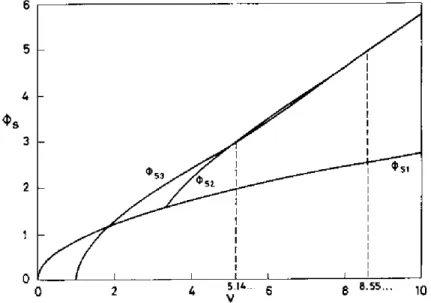
where a and 6 are as defined in (3.15). A plot of the first coordínate of the points 1, 2, and 3 (the last two of them as defined above) is given Fig. 5. If 0 < e S 1 and B>0, then points 2 and 3 do not exist. If 1< v < va = 1.8466 • - -, then *s 3 < <t>vl, while, if v> v0, then *s 3> * . t i - The plots of <J>s2 and <í>s3 (the latter exists only if v> 10/3)

intersect infinitely often, for a sequence of valúes of v, p, = 5.1482 • - • < v2 = 8.5523 • <v3<v4<- • ,asseenbyanasymptoticanalysisofthesystems(3.17)-(3.18) and (3.22), (3.23); the asymptotic behavior of vk is given by

Vk (kir + A695- • - ) x 1.0857- • - + o(l) as fc^-oo.

From these properties the following conclusions hold:

(i) If B>0 and 0 < c S l , then the curve C'2 intersect neither the curve C\ ñor the curve C2 (that is below the curve CL).

8.55.

0 2 4 *•'*- 6 8 ° " " 10 F i e . 5. The first coordínate of points 1, 2, and 3 in Fig. 4 in terms of

v-(ii) If B > 0 and 1< v < v0 = 1.8446 - - •, then the situation is as in one of the sketches (a) or (b) of Fig. 4. The curve C2 intersect the curve C, (at p3), but it does

not necessarily intersect the curve C2 (since í >3 l> Oj 3 and the curve C2 is below the curve C2 for sufficiently small 4>s).

with í l / 0. This is a codimension-three degeneracy that has been partially analyzed in [12], where it has been shown that it leads to bifurcation to two- and three-dimensional tori, That degeneracy corresponds to the following situation: a Hopf bifurcation point crosses one of the bending points 1 or 2 of the response curve of Fig. 1 and, simultaneously, that bending point exhibits a saddle-node degeneracy.

{iv) If B > 0 and v0< ^ = 10/3 (respectively if 10/3< f < v¡ or, more generally,

if 1'2k< v< v?k+\ for some fc= 1), then the situation is as in one of the sketches (c) or

(d) (respectively, (e) or (f)) of Fig. 3. Therefore, if vB < v < v,, then the curves C> and C'2 intersect at (at least) a point p¿,. At p4 the linearized problem around the steady

state possesses two pairs of complex conjúgate simple eigenvalues CÚ = ±ÍÍÍ, and oí = ± í í l2, w i t h í l! ^ 0 and n2; ¿ 0 . This isa codimension-two singularity whose universal

unfolding has been completely analyzed [9]; in particular, it is known that the degeneracy leads to bifurcation to tori. The degeneracy corresponds to the following situation: two Hopf bifurcation points, with linearly independent eigenspaces, coalesce.

(v) If B > 0 and v — vx (or, more generally, v — vk for some fe> 1), then the points p2 and p3 coalesce. At the resulting point, the linearized problem around the steady

state has a simple zero eigenvalue at =0 and two pairs of complex conjúgate simple eigenvalues w = ± i'íl, and <o = ± iü2, with í l , ^ 0 and íí2 ^ 0. This is a codimension-three

degeneracy that has been partially analyzed in [13] and leads to bifurcation to two-and three-dimensional tori. It corresponds to the following situation: two Hopf bifurca-tion points, of linearly independent eigenspaces, simultaneously cross one of the bending points 1 or 2 of the response curve of Fig. 1.

(vi) If B>Q and v2k-í < v< v2k for some fe^l, then the situation is as in one of

the sketches (g) or (h) of Fig. 4. Observe that the curves C2 and C2 intersect at a point

j>4, where a degeneracy of codimension-two (namely, that appearing in case (iv)) takes

place. Nevertheless, that degeneracy appears now at a point of the middle branch of the S-shaped part of the response curve of Fig. 1, where the linearized problem around the steady state has a real eigenvalue that is strictly positive. Therefore, no attractor of the dynamical system definedby (3.1)-(3.4) can bifúrcate from the steady state near that singularity. Thus it is not of much interest.

To summarize the above results, the following degeneracies of codimensions two and three, leading to quasi-periodic behavior of (3.1)-{3.4), have been found above (CÜ] , <¡>2, • • • are the eigenvalues of the linearized problem around the steady state with

zero real part):

(i) wj=0, <w2j3 = ± í í l , with fí?¿0;

(ii) (¡>i2= ±iSíi,a>J:4 = ±i(l2 with íl, ;¿0 and í l2^ 0;

(iii) to, = 0 (algebraically triple, geometrically simple);

(iv) £D, = 0 (algebraically double, geometrically simple), a>2t3 = ±¿íí with f i ^ O ;

(v) w, = 0 , <ií2>3 = ± í í i i , a)4p; = ±¿íi2,with fii ^ 0 and íi2 ?* 0.

Finally, observe that the stability analysis above, of the spatially one-dimensional problem (3.1)-(3.4), must be seen with some caution from the physical point of view, since the real world is three-dimensional. That analysis is expected to apply to the three-dimensional versión of {3.1 )-(3.4) in í l = ] - 1,1[ x í l , , where í l , <= u2 is a bounded

domain, if the boundary conditions (3.2) are imposed at { —1,1} x í l , , Neumann boundary conditions are imposed at ] - l , l [ x d f i i , and the domain íli is sufficiently small; this should be seen by extending well-known results by Conway, Hoff, and Smoller [24]. This, however, is not true if the domain í l , is sufficiently large; in that case, we expect additional degeneracies of the linear stability problem, of codimension greater than three. In the limiting case in which í l is an infinite slab, a new source of chaotic behavior appears, namely, the so-called phase turbulence [25]. We do not pursue this important question any further in this paper,

4. Quasi-periodíc and other eomplex phenomena for tnodel 2 in one dimensión. In this section we analyze {via local bifurcation theory) the model (3.1)-(3.4) near a point of the parameter space (<t>, y, v, B) = (<t>0, y<\, v0, B0), where the Hnearized problem

around a uniform steady state (us(), vs¡>) exhibits the degeneracy (í) encountered in § 3.

Recall that this degeneracy corresponds to the interaction of a Hopf bifurcation point and a bending point of the response curve. The analysis will be made by reducing the problem to a three-dimensional center manifold and obtaining its normal form; then we use the general analysis of this normal form in [9]. Let us mention that similar (but different) normal forms are obtained at the interaction of a Hopf bifurcation point and either a transcritical or a pitchfork steady bifurcation point; see [26], [27] and also [9, pp. 396 and 410].

We take <t>0, Yo, f0, and B0 such that (3.12)-(3.18) hold for some positive valúes

ofthe real parameters í l = í l0 and $>s = <5j0, where <!>,<, satisfies (3.9). Then the linearized

problem around the steady state (3.8) has the simple eigenvalues ta — iíl0, w = — ííl0,

and w= 0 , with (V, U+, U_) = ( V,, Ul+, l/,_), {V,, Ül+, Ü,_), and {V2, U2+, U2_) as

associated eigenvectors, where (here and below) overbars denote eomplex conjugation, and

(4.1) V,(x) = cosh{ViíVc)/cosh{v7ñ¡), V2(x) = l i n - l g j c S l ;

t /l +( í ) = t / i - ( í ) = Tü^ü^'üCexp ( ^ i ñ ¡ f ) - e x p ( *í 0f í l / i f t o í ^ + S * ^ )2,

(4.2)

^+{ f ) = ^ - ( í ) = 7 o ^ , o í e x p { *i üí ) / 2 (1-ü+ B0*s 0)2 in - o o < ^ S 0 .

In addition, we assume that

(4-3) <t>s0

^o/Bo-This condition and (3.12) mean that the steady state under consideration is, in fact, one of the bending points 1 o r 2 ofthe response curve of Fig. 1. If (4.3) does not hold, but conditions (3.9), (3.12), (3.17), (3.18) are still imposed, then the steady state bifurcation diagram exhibits the cusp degeneracy (which corresponds to coalescence of the bending points 1 and 2), and the local dynamic problem presents a degeneracy of codimension-three that will not be considered here.

Now let the parameters v, B, y, and Q2 be cióse to v0, B0, y0, and <t>l, and let

the parameters s = ( £ [ , g,, e3)eí(53 and SeU be defined by

v=v0+ei, B=B0+e2í y = 2[v + B{<b;0+e1)flvB(Q>,íi+E,),

(4.4)

Note that O, B, y, 4>2)->(r0, BQ, y0, *ü) as |e|2 + 53^ 0 , and that the map (e,á)-»

(v, B, % $>2) defined by (4.4) is one-to-one if je|2+ S1 is sufficiently small (its Jacobian

at |e| = d = 0is diíferent fromzero according to condition (4.3)). The parameters e and 8 are defined in such a way that if S = 0 and |e¡ is sufficiently small, then (3.1)-(3.4) possess the steady state

v¿e) = [v + B ( *s 0+ e3)]/v, us +(£ «)».«-(£ e) = e x p [ ( * ,0 + e3)£|

(4.5) . , „ i n - o o < £ < 0 .

Also, (i) vs, M3+, and w3_ depend smoothly on e; (ü) (i>„ w.tdt)-»(uso> «io±) (— the basic

steady state that we are considering) as e -> 0 and 5^-0; and (iii) the linearized problem around the steady state (4.5) possesses the eigenvalue w = 0 (for all e such that |ej is sufficiently small).

Now, if |e|2 + S2 is sufficiently small, we consider a three-dimenstonalcenter manifold

of the phase space of (3.1)-{3,4), M(S>5), which is invariant under the semiflow defined

by (3.1)-(3.4). AÍ(S,S) is defined in a neighborhood of the steady state (DJ 0, «SO+, «JO •),

and AÍ(0Ü> contains that steady state and is tangent {at the steady state) to the linear

manifold spanned by the eigenvectors (of the linearized problem) associated with the eigenvalues fO0, —iíl0, and 0. In addition, we require Mi0¡f:) to contain the steady state

(4.5) (for |e| sufficiently small). Aí( 6 f ) may be represented parametrically (through the

parameters a e C and j3 e R) as

(4.6) v(x) = VÍ(E) + aVl(x) + áV,(x) + BV2(x)+ V(x; a, átB;8,e),

(4.7) u±(0 = usJí,e) + aUlJe + ¿ÜiJ£) + 8U2Jt)+ܱ(£;a,á,8-8,e).

Here Vjt Uj+, Uj- (for j= 1 and 2), vs, uF+, and w^- are as given by (4.1), (4.2), (4.5),

and the functions V[-l, l]xS8-»R and Ü+, (/_:]-<», 0 ] x 3 3 ^ R (for some neighbor-hood Si of the origin of C2 x U5) depend smoothly on x or ¿ a;R, a,, B, 8, and e, where

(4.8) aR = Re a and a, = Im a.

In addition, V", Ü+, and 0- satisfy the determinancy conditions •o

(4.9) i VVfdx+\ Ü+Uf+d£- U- Uf- d$ = 0 for j = 1 and 2,

*• ' r rst / *-\ _ T r *

where (Vf, t/f+, [/*_) and (V$, Uf+, U*~) are eigenvectors of the adjoint linearized problem associated with the eigenvalues iíl0 and 0, i.e.,

(4.10) VT(x) - (*ío+ íílo) cosh (vTfi^c), VJ(JC) = 1 in - 1 == x S 1, l / f+( í ) - £/f_(í)= So*'ocosh ( v ^ K I - e x p ( V ^ + i í U ) ] ,

U ?+( í ) - t / í - ( f ) = f l0[ l - e x p ( *í Of ) ] i n - o o < £ £ 0 .

Also, the steady state (4.5) is assumed to correspond to a = 0, 8 = 0 if 5 = 0, i.e., (4.12) V=0, Ü+= Ü_ = 0 i f a = j 3 = S = 0.

As a consequence of conditions (4.9) and (4.12), it may be seen that the following tangency conditions hold:

d V/da = d V/dá = dV¡dB = 0,

dÜJda = dÜJdá=dÜJd8 = 0 if a =0,/3 = 0, and e=0,

where ó/da and 3/<?<5 are the formal (V, Ü+, and í/_ are not necessarily holomorphic) partial derivative operators, defined by (see (4.8))

Now the restriction of the semiflow defined by (3.1)-(3.4) to the center manifold may be described by a fhird-order real {when decomplexified) system of ODEs of the form

(4.14) da/dt=f(atátp;8,E), d8¡dt = g{a, a, B; S, e),

for some functions, /:í53-»C and g:$S-*U {for some neighborhood £8 of the origin of C2xlR5) that depend smoothly on aR, a, (see (4.8)), j3, 5, and e. These functions

are determined (together with the functions V, Ü+, and t/_ defined above), at least locally, by the problem posed by (4.9), (4.12), and (4.15)-(4.18) below, which are readily obtained by imposing the invariance of the center manifold under the semiflow defined by (3.l)-(3.4):

(4.15) 3lV/dx2 = (Vl + dV/da)f+(í+dV/dp)g-iCloaVl + c.c. i n - l < x < l , dV/dx= *a-fiíí¿ta.nhVíCht±v{-B®¡/v-a-p- V]

(4.16) ± B4>2 exp [y - y/(u.,. + a + á + 8 + t>)]

[ut + aU]± + BU2±+U±] dg + cc. at x = ± l , J — ÜO

d2ÜJd? = (Ul±+dÜJda)f+(U2±+dÜJdB)g-ad2UlJdf-Bd2U2Jdf-<!>2u¡

(4.17) +<t>2(us + aU,* + 8U2*+ ܱ) exp[y - y/ (v3 + a + á + 8 + VJl + cx. in -oo < £ < O,

(4.18) t>± = 0 at £ = - o o a n d e = 0 .

Here V±= V(±l; a, á, 8\ S, g), d/da is the operator defined in (4.13) and c.c. denotes

the complex conjúgate.

The problem posed by (4.9), (4.12), (4.15)-(4.18) may be solved by (regular) perturbation techniques, by seeking the asymptotic expansions (p, q,r,s = nonnegative integers)

/ ( a , á , j 8 ; a , e ) = I l f^(e,S)a"a'B\

p q-\-r-t2=-p

g{a,á,B;Bte) = X I ^ ( e , 8)a"árB',

(4.19)

j £jrs\

p q + r+s*=tp

V(x; a, 5,8; £ E) = 1 I V^Jx; 8, B)a"árB\ p q+r+s=p

ÜM a, a,B; S, e) = 1 E Ú £ ^ ( x ; 8, s)a«á'B\ p q+r+R=p

The coefficients are uniquely determined from the system of recursive linear problems that results when the expansions (4.19) are substituted into (4.9), (4.12), (4.15)-(4.18), and the coefficient of each monomial a"á'Bs is set to zero. Below, we consider all

coefficients up to order p = 3 in the expansions of / and g, but we must explicitly compute only a first approximation of the following:

g0US,e) = Ao8 + 0(82 + \e\2)

Re[/,!oo(0, e)] = A,gl + A2e2 + A,1e3 + 0(|e|2) ( 4-2 0 ) Im[/1'O0(0,0)] = no,

Re[/2 0 1(0,0)] = A4, gí,o(0,0) = As, g202(0,0) = A „

where the constants A0, • • • •, A6 are given in the Appendix B.

replace the resulting polynomial in (4.14). Then we consider a near-identity change of variables (a,p)->(y{a,p; S, e), z(a, 0 ; 8, e ) ) e C X 03, with y-a and z~¡3 as ( a , 0 , S, e ) ^ (0,0,0,0), of the form

(4.21) y=Z I V ^ ( « , « ) a ' o ' j 8, 1 z = ¿ £ Z ^ ( á , « ) « * « ? ' ,

whose coefficients are selected in such a way that, in the new variables, system (4.14) becomes of the form

dy/dt = [a0(8,E)+k0(8, e)]y + [a1(S,e) + icl(8, s)]yz

+ [^(8>E) + icMs)]y2y + [ai(8,e) + icí(8,e)]yz2+0(\y\2+z2)2, dz/di = b<i(8,e) + bl(8,e)yy + b2(S,s)z2 + bi(5,s)yyz

] +b4(8iE)z3 + 0(\y\1+z2)\

where the real coefficients a,, fe,, and c, are such that

b<,(8,E) = A0S + O(\e\2 + 82), a0(0, e) = Alel + A2e2 + A1s-l + 0(\e\2), (4 24)

í*(0,0) = í lu, al{0,0) + icl(Q,0) = A4, 6,(0,0) = AS, b2(0,Q) = A6.

The terms appearing in the right-hand side of (4.22) cannot be annihilated by a change of variables of the type (4.21), and are called resonants.

That change of variables is seen to exist by applying the implicit function theorem to the system of equations that results when (4.21) is substituted into (4.14), and the coefficient of the monomials not appearing in (4.22) is set to zero (observe that g w2( 0 , 0 ) / 0 ; see (4.3) and (4.20)).

Now, when the new real variables r > 0 and 0, defined by y = rexp(i$) are introduced, (4.22) is written in the form

(4.25) drjdt = aar + alrz + a2r3 + a3rz2+0(r2+z2),

(4.26) dz/dt^ba+b^ + b^ + b^z + b^ + OiS + z2)2,

(4.27) d0/df = c:o + c,z + (;2r2 + C322+O{r2 + z2

)7'--Then (4.25), (4.26) are decoupled from (4.27), and they may be solved separately. Note that the stationary (respectively, periodic) solutions of (4.25), (4.26) with r> 0 are periodic (respectively, quasi-periodic) solutions of (4.25)-(4.27). Now we may use the fairly complete analysis of (4.25), (4.26) made in [9, pp. 376-396], To this end, we first reduce (4.23), (4.25) to standard form by using the new variables and parameters

w = \b,/b2\U2r, v = -b2zy ¿i, = aa, fi2 = -bBb2, a = -ajb2,

(4.28) fe = - s i g n [ b2/ f > , ] ( = ± l ) , c = a2b22/b2, d = a^/b22i e = b¡b,/b2, f=bjb22

to write (4.25), (4.26) as

du/dt = filu + auv + cui + duv2+0(u2 + v2)2,

( 4'2 9 ) dv/dt = ^2 + bu2-v2 + eu2v+fv1 + 0{u2+v2)2.

Here we assume that fe, ^ 0 (note that b2 # 0; see (4.3), (4.20)).

Now, when using (4.24), (4.28) and the expressions for A0, .4.,, A2, and A3 in

Appendix B, it is seen that the map (5, e)-*(/j,J(8, e), ju,2(S, e)) of R4 into U2 is such

that the rank of its Jacobian matrix at (8, e) = (0,0) is always equal to 2. As a consequence, any point (¿Í.L , ft2) in a whole neighborhood of the origin of U2 may be

From the analysis in [9], if a<0 and 6 = 1, then system (4.29) exhibits a Hopf bifurcation at a curve of the plañe /u, - /x2 (for fixed valúes of the remaining parameters)

of the forra ¿i, = fj-i{f¿2)', with M2<0> such that ^ í ( 0 ) = 0 . At that curve, the original

problem exhibits a bifurcation to torus; it is well known (see, e.g., [10, pp. 292-313]) that, when having at least two free parameters (we have four of them available), near that bifurcation the dynamical system exhibits a quite complex dynamic behavior, which includes a large number of periodic solutions and, quite frequently, chaotic behavior. Also, if a>0 and f> = - 1 , then near a curve of the plañe / ¿ , - ¿ A2, of the type

JLI, = MIÍMÍ), wit n Mz > 0> system (4.29) presents a homoclinic bifurcation that is expected

to yield also quite complex dynamic behavior for the original system (see, e.g., [9, p.394]). Both situations ( a < 0 , b = l and <a>0, ¿> = - l ) do occur for appropriate valúes of the parameters in our case, as it comes from the plot in Fig. 6, where the curves Re(A4) = 0, A5 = 0, and A6 = 0 are represented in terms of B and v (the

expressions of A4t A5, and Aft in Appendix B depend on the parameters O, <f>s, B,

and vt but <¿\- and íl are eliminated when using (3.17), (3.18)). These curves define

several regions in the plañe v — B. In particular, in región I, Re ( A4) > 0 , A5<0, A6> 0 ,

and {see (4.24), (4.28)) the parameters a and b are such that a< 0 and ft = 1; similarly, in región II, R e ( A4) < 0 , /45<0, A6<0, a>0, and ¿ = - 1 . Note that a blow-up of the

región near the point v — 10/3, B - 2-/10/3 is necessary to appreciate a second point of intersection of the curves Re (A4) = 0 and As = 0.

5. Conclusions. We have obtained two realistic submodels of (1.1), (1.2) in the limit (1.3) for v~\, which we cali models 1 and 2. Their formal derivationby singular perturbation techniques, was made in Appendix A and § 2.

F I G . 6. Tke curves Re (J44) = 0, ,43 = 0, and Af, = 0.

parameters, the dynamics of the model is quite rich. Those results lead us to the conjecture that model 2 should present chaotic behavior for appropriate valúes of the parameters.

Since, as we explained in § 1, model 2 is obtained in a realistic limit, we expect that the results in this paper explain some experimentally observed, quite rich dynamic behavior under apparently isothermal conditions; see, e.g., [28], [29], and [1, Vol. II, pp. 140-141], Finally, to our knowledge, model 2 is the first submodel of (1.1), (1.2) in the literature such that (a) it is obtained for realistic limiting valúes of the parameters, (b) it is simpler than (1.1), (1.2), and (c) it exhibits generically stable quasi-periodic behavior.

Appendix A, Asymptotic derivation of the basic model. In this appendix we consider the Hmit {1.5} with v~\, for the problem (1.1), (1.2), with initial conditions

(A.l) u(x,Q) = Ü(x)>Q, v(x,Q) = v{x)>0 in O,

where the smooth functions ü and v satisfy the boundary conditions at dfl. For brevity, only the spatially three-dimensional case is considered, but the results of this section are also valid in one and two space dimensions. AIso, for simplicity in the presentation, weassumethat y ~ O(l). Again, it may be seen that the basic model applies also if y » 1 .

Below, we encounter two thin boundary layers beside the boundary of íi. To describe íhe (inner) solution in these layers, we introduce, in a neighborhood B of each point of díl, a curvilinear coordínate system {17, 17,, ij2) such that d(l is the

parametric surface r¡ — 0 and r¡ is a coordínate along the outward unit normal to díl, Then the Laplacian operator is written as

A = d2/d7}2 + hiid2/dvidvJ+ pd/dV + pkB/dv\

where h'', p, and pk{i,j, k — 1 and 2) are appropriate smooth functions defined in the

neighborhood B.

Two timescales must be considered. For í — l/cr, a boundary layer of thickness 1/vo- appears beside the boundary of the domain. We use the time variable r = trt and the inner variables £ = \/CT7J, TJ2, and 773 in the boundary layer, and we seek the

expansions

w = W0+ U1/ \ / C T + - • • , i> = ü0 + i ? i / \ / í r + - • •

in the outer zone, and of the form

u - M0+ií]/Vc^+• * •, u = vQ+ví/\ío:+- • •

in the boundary layer. Then uQ and t>0 are given by

(A.2) Kdujdr = 0, M0{X, y, 2; 0) = t¡(x, y, z),

(A.3) dvJdT = b<p2u0exp ( y - y/v0), va(x, y, z; 0) = v(x, y, z),

and M0 and v0 are given by

(A.4) \düjdr = 0, ü0(l V\ r¡\ 0) = w(0, TJ', r,2),

ÍA.5) dv0/dT = d2v0/dg2 + b<p2ü(te\v{7-y/vü), óvJd^O at £ = 0,

(A.6) vo(Z,vl,v2;0) = v(o,v\v2),

where the parameters A, b, and <p2 are as defined in (1.11). By uniqueness of solution

of (A.4)-(A.6), we obtain that neither w0 ñor DU depend on i. Then v0 is given by

and, to the leading order, the boundary layer can be ignored at this time stage, since the inner problem (A.4), (A.6), (A.7) is obtained by writing the outer probiem in the inner variables. This is no longer true for higher-order terms, since, for example, ü' does depend on $ for T > 0 , as is easily seen.

The behavior of w0 and u0 as T-* OO is easily obtained, from (A.2)-(A3), to be

w0 = w, va = b(p2ü exp(y)T + 0 { l ) in íí.

Therefore v^ — tT as r •— a, and we are led to the following time stage for t •— 1. Now a new boundary layer of thickness 1/a- appears beside díl. We use the inner variables t= Va, v\ a nd V2 m this new boundary layer, and seek expansions of the form

in the outer zone, of the form

in the first boundary layer (of thickness 1/VCT), and of the form U — M0+ M1/ v/o:+ M2/ o ' + - • - , l> = crVo + V c r V i + V2 +' • '

in the second boundary layer (of thickness 1/tr). Then w0 and V0 are given by

(A.8) \dujdt = -<P2U0 exp (y),

(A.9) aV0/áí = AVo+fxp2woexp(y);

w0s Vg, and V, are given by

(A.10) kdüjdt = -<p2ü0 exp {-y),

(A.11) d2VJdf = d1VJc)? = 0;

and «u, V0, Vly and V2 are given by

(A.12) Xdüjdt = &2üJdC2-<P2^ exp (y); düo/dZ = 1 - fl0 at f = O,

(A.13) á*Vo/tt

= ¿

Vi/tt

= 0; d^o/aí = a^i/aí = o at£ = o,

We do not write the initial conditions for the above problem, which come from matching conditions wifh the earlier time stage. From (A.13), we obtain that neither V"0 ñor Vx

depend on £, and (A.14) yields BV^/Bl = -vVa in - o o < £ < 0 . Then, from (A.11) and

matching conditions between the two boundary layers, we obtain that V0 does not

depend on £, and dVJdg = — uV0 in — o o < £ < 0 . Finally, matching conditions between

the outer zone and the first boundary layer yield

(A.15) dVJdn = -vV0 a t a n .

Now, from (A.8) and (A.10), we obtain that «o-»0, M0- » 0 as í-»°os and then (A.9) and

(A.15) yield V0-*0 as f-*oo. In the same way, from the equations giving higher-order

terms, which are not written for brevity, we obtain that, as r-»oo, v — 0{\) everywhere in n , and w = 0(1/0-) in the outer zone and in the first boundary layer. Therefore, for sufficiently large í,

u = o(l/or), dv/dt=Av + o(l)

both in the outer zone and in the first boundary layer, and fhese two zones need not be distinguished in first approximation. Then, if we seek the expansions D = v0+vf/-/a+- • •, in the outer zone, and

in the second boundary layer, vB satisfies {1.7}, uQ satisfies (1.9), (1.10), and ¿30, vlt

and v2 are given by

(A.16)

á

%lac

= aHjac

= ^ dV

/a£ = as

/ac = o a t í = o,

Then neither Ü0 ñor ü, depend on £, and, by integrating (A.16) from -oo to 0, we

obtain that

dvJH = v{\-v(S) + b<p1e\p{y- y / v0) üo(£,r) d( as £-»-°o.

Then matching conditions between the outer zone and the boundary layer show that Uo satisfies (1.8) at 5Í1, and the derivation of (1.7)-(1.10) is complete.

Finally, observe that if the nonlinearity <¡>2u exp {y — y/v) is replaced in (1.1),

(1.2) by a more general one, <j>2f(u, v), w h e r e / i s a nonnegative smooth function such

that /(O, v) = Ú, then the above analysis stands after obvious changes. The resulting model is that obtained from model 1 by replacing the terms <p2 exp (y - y¡ v) \ \ u(C, t) di and <p2u exp (y- y/v) by <p2 £ „ / ( « < £ t),v(t)) di and <p2f(u, v) in (1.7)

and (1.8), respectively.

Appendíx B. The valúes of the constants A0fAít---A6 that appear in (4.20) are

as follows:

Aa =

2fi4>?

4 ^ ( 4 * ; - 3 v) > 0 ,

A , =

-- 7 £ *J- 3 í ' + - ( 3 B < J >I + i 0 v i í l t a n h V i í i

( B í . + vJC, ' 2f(B4>

A,=-- 2 ( f i ^ A,=--t- ( l + 2 4 >J) ) + 2^B 4 > I + i" ' Y - F — - — - ( & . - t Ü ) ) + - v ^ n t a n h V 7 n

¿fifi V<í>2-ifi / e

( S Í . + vJC,

^ =

2 (y( l + 2B ) - B ^ + (( 8 f n + 2*y' + y ) + 4 B 0J- K l+2 ^ ) ) ^ t a n h V f ñ

( B *r+ » - ) C i

fíí V *2+ i " í l /

( B *t + ^)C,

6¿>

2 ^ , /2«E>2+;ft)(B<Í>, + ^ , . „ \ t a n h

Á B *s V B * , / VT

^ 4 = , „ , , T ^

t a n h v/í n

V7H

( B ^ + W C

2 ^

A,=

4 * ^ — + - - -b 2/ V 2 ñ (sirihV2fl + siriV2fl)\\ Ví>í + íl2J 'V Ü ( c o s h v ^ + c o s V S ñ ) / /

B(4$*-3v)

4&sv2(B<í>s-v)

6~B(B<frt+K)(4<l^-3K)'

where

_^/tanhvfiíí

C,=

2 \ vTñ

**2

l+cosh2 vTn/

"*í

( * ; + ¡ Í « 3/2 ( * , W *2+ Í Í I )3.

* , + 2V*f+íñ

( *2+ i f l )V 2L ( * . W *2+ ¡ f i )2

Here the suffix 0 has been dropped out everywhere from the parameters Ba, v0,

0jOí and íí0, which are defined at the beginning of § 4 and b is defined in (3.15).

REFERENCES

[1] R. A R I S , The Mathematical Theory of Díffusion and Reaction in Permeable Catalysts, Vols. I and II, Clarendon Press, Oxford, UK, 1975.

[2] N. R. A M U N D S O N A N D L. R. R A Y M O N D , Stability in distributed parameter systems, Amer. Inst. Chem. Engrg., H (1965), pp. 339-350.

[3] I. E. PARRA A N O J. M. VEGA, Local nonlinear stability of the steady states in an isothermal catalyst, SIAM J. Appl. Math., 48 (1988), pp. 854-881.

[4] J. M. VEGA, Invariant regions and global asymptotic stability in an isothermal catalyst, SIAM J. Math. Anal., 19 (1988), pp. 774-796.

[5] R. Hu, V, BALAKOTAIAH, A N D D. LUSS, Multiplicity features ofporous catalyticpellets, Part 1: Single

zeroth-order reaction case, Chem. Engrg, Sci., 40 (1985), pp. 589-598; Part II: Influence of reaction arder and pellet geometry, Chem. Engrg. Sci., 40 (1985), pp. 599-610; Part III: Uniqueness criterio for the lumped thermal model, Chem. Engrg. Sci., 41 (1986), pp. 1535-1537.

[6] P. L. L I O N S , On the existence ofpositive solulions of semilinear ellíptic equations, SIAM Rev., 24 (1982), pp.441-467.

[7] J. K., H A L E , Asymptotic Behavior of Dissipative Systems, American Mathematical Society, Providence, RI, 1988.

[8] L. M. P I S ' M E N A N D Y. I. K H A R K A T S , Asymmeiric state of a heterogeneous exothermic reaction, Dokl. Akad. Sci. USSR, Chemical Technology Section, 178/179 (1968).

[9] J. G U C K E N H E I M E R A N D P. H O L M E S , Nonlinear Oscillations, Dynamical Systems and Bifurcations of

Vector Fields, Springer-Verlag, Berlín, New York, 1983.

[10] V. I. A R N O L U , Geometrical Methods in the Theory of Ordinary Differenttal Equations, Springer-Verlag, Berlín, New York, 1983.

[11] P. Yu A N D K.. H U S E Y I N , Bifurcations associated with a three-fold zero eigenvahte, Quart. Appl. Math., 46(1988), pp. 193-216.

[12] , Bifurcation associated with a double zero and a pair of puré imaginary eigenvalues, SIAM J. Appl. Math., 48(1988), pp. 229-261.

[13] K., HusEYtN A N D P. Yu, Bifurcation associated with a simple zero and two pairs of puré imaginary

eigenvalues, in CMS/AMS Proc. Interna!. Conf. on Oscillation, Bifurcation and Chaos, Toronto,

Ontario, Canadá, 8 (1986), pp. 465-484.

[14] L. M. PIS'MEN, Methods of singularity theory in the analysis of dynamics of reactive systems, in Lecture Notes in Appl. Math., Vol. 24-11, American Mathematical Society, Providence, RI, 1986. [15] J. B. PLANEAUX, K. F. J E N S E N , A N D W . W. FARR, Dynamic behavior ofcontinuous stirred-lank reactors

with extraneous thermal capacilance, in Lecture Notes in Appl. Math., Vol, 24-11, American

[16] D. Luss, J. E. BAJLEY, A N D S. S H A R M A , Asymmetric steady states in catatytic slabs with uniform and

non-uniform environment, Chem. Engrg. Sci., 27 (1972), pp. 1555-1567.

[17] D. G. A R O N S O N A N D L. A. PÍÍLETIER, Global stabilily of symmetric and asymmetric concentration

profiles In catalyticparticles, Arch. Rat. Mech. Anal., 54 (1974), pp. 175-204.

[18] D. O. A R O N S O N , A comparison method far stability analysis of nonlinear parabolic problems, SIAM Rev., 20 (1978), pp. 245-264.

[19] J. M. B A L L A N D L . A. PELETIER, Stabilization ofconcentration profiles in catalyst particles, J. Differential Equations, 20 (1976), pp. 356-368.

[20] N. D. A L I K A K O S , Quantitaíive máximum principies and sírongly coupled gradient-Uke reaction-diffusion

systems, Prac. Roy. Soc. Edinburgh, 94A (1983), pp, 265-286.

[21] F. J. M A N C E B O A N D JL M. VEGA, Global analysis of a model ofporous catalyst, 1992, in prepararon. [22] S. N. C H O W A N D J. K. H A L E , Methods of Bifurcation Theory, Springer-Verlag, Berlin, New York, 1982. [23] F. J. M A N C R B O , Efectos térmicos incipientes en catalizadores porosos, Tesis Doctoral, Universidad

Politécnica de Madrid, Madrid, Spaín, 1992.

[24] E. C O N W A Y , D. H O F F , A N D J. SMOLLER, Large-time behavior of solutions of systems of nonlinear

reaction-diffusion equation, SIAM J. Appl, Math., 35 (1978), pp. 1-16.

[25] Y. K U R A M O T O , Chemical Oscillations, Waves and Turbulence, Springer-Verlag, Berlin, New York, 1984. [26] W. F. L A N O F O R D , Periodic and steady made Interaction lead to tori, SIAM J. Appl. Math., 37 (1979),

pp. 22-48.

[27] G. l o o s s A N D W. F. L A N G F O R D , Conjectures and the routes to turbulence via bifurcation, in Nonlinear Dynamics, R. H. G. Helleman, ed., New York Academy of Sciences, New York, 1980, pp. 489-505. [28] P. F I E G U T H A N D E. WECKE, Der Übergang vom ZündjLosch-Verhalten zu stabilen Reaktionszustánden

bei einem adiabaiischen Rohrreaktor, Cheime-Ingr-Tech, 43 (1971), pp. 604-608.

[29] H. B E U S C H , P. F I E G U T H , A N D E, W I C K E , Unstable behavior of chemical reactions at single catalyst

particles, in Proc. First Internat. Conf. on Chemical Reaction Engineering, Washington, DC, 1970,

American Chemical Society, Washington, DC, pp. 615-621.

[30] F. J. M A N C E B O A N D J. M. VEGA, An asymptotic justificaron ofa model of isothermal catalyst, J. Math. Anal. Appl., 1992, to appear.

[31] A. ui LLDDO A N D L. M A D D A L E N A , Mathematkal analysis of a chemical reaction with lumped