Abstract
This paper presents a time-domain stochastic system identification method based on Maximum Likelihood Estimation (MLE) with the Expectation Maximization (EM) al-gorithm. The effectiveness of this structural identification method is evaluated through numerical simulation in the context of the ASCE benchmark problem on structural health monitoring. Modal parameters (eigenfrequencies, damping ratios and mode shapes) of the benchmark structure have been estimated using both Stochastic Sub-space Identification (SSI) method and the proposed MLE+EM method. The numerical results show that the proposed method estimates more accurate modal parameters than SSI in the presence of 10% measurement noise. Finally, adventages and disadventages of the method have been discussed.
Keywords: system identification in structures, state space models, Kalman filter, stochastic subspace methods, modal analysis, benchmark problems.
1
Introduction
The application of system identification to vibrating structures consist in identifying a modal model (eigenfrequencies, damping ratios and mode shapes) from vibration data. Classically, a measurable input is applied to the system and the output is mea-sured. From these experimental data, a system model can be obtained by a variety of parameter estimation methods, and it is known as experimental modal analysis. How-ever, cases exist where it is practically impossible to measure the excitation and the outputs are the only information that is passed to the system identification algorithms. In these cases the deterministic knowledge of the input is replaced by the assumption that the input is a realization of a stochastic process (white noise), and it is known as stochastic system identification (the terms output-only modal analysis and operational
Paper
66
Maximum Likelihood Estimation of Modal Parameters in
Structures Using the Expectation Maximization Algorithm
F.J. Cara1, J. Carpio1, J. Juan1 and E. Alarcon2 1 Department of Organization Engineering,
Business Administration and Statistics
2 Department of Structural Mechanics and Industrial Constructions
Polytechnical University of Madrid, Spain
©Civil-Comp Press, 2010
modal analysis are used as well).
Parametric structural identification methods involve the use of mathematical mo-dels to represent structural system behavior in either time or frequency domain. The benefits of using parametric models for structural identification include their direct re-lationship with physically meaningful quantities such as stiffness and mass, improved accuracy and resolution, and their suitability for analysis, prediction, fault diagnosis and control.
Popular time domain parametric models used for structural identification purposes include: ARX models, ARMAX models, state space models, etc. Many identification algorithms are available to estimate the parameters of such parametric models, e.g. prediction error method (PEM), least squares estimation (LSE), maximum likelihood algorithm (MLA), eigensystem realization algorithm (ERA) and stochastic subspace identification method (SSI).
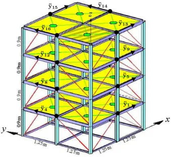
This paper presents a time-domain stochastic system identification method based on Maximum Likelihood Estimation (MLE) with the Expectation Maximization (EM) algorithm. The effectiveness of this structural identification method is evaluated through numerical simulation in the context of the ASCE benchmark problem on structural health monitoring [7]. Modal parameters (eigenfrequencies, damping ratios and mode shapes) of the benchmark structure (see Figure 2) have been estimated using both Stochastic Subspace Identification (SSI) method and the proposed MLE+EM method. SSI identification method is a well known method and computes accurate estimates of the modal parameters ([9], [10]), and for this reason it has been used for compar-ison. The principles of the SSI method have been introduced in the paper and next the proposed Maximum Likelihood Estimation with Expectation Maximization algo-rithm has been explained in detail. Finally, the results obtained with both methods are compared.
2
State space model
A vibrating structure can be represented by a discrete-time stochastic state-space model given as:
xk+1=Axk+Buk+wk yk =Cxk+Duk+vk
(1)
where
kdenotes the sampling instant (t =k∆t, with constant sampling time∆t);
yk∈Rlis the measured output vector;
uk ∈Rmis the measured input vector;
xk ∈Rnis the discrete state vector;
vk∈Rlis the measurement noise due to sensor inaccuracy
A ∈ Rn×n is the transition state matrix describing the dynamics of the system (as
characterised by its eigenvalues);
B ∈Rn×mis the input matrix;
C ∈ Rl×n is the output matrix, which is describing how the internal state is
trans-ferred to the the output measurementsyk;
D∈Rl×mis the direct transmission matrix;
The noise vectors comprise unmeasurable vector signals assumed to be zero-mean with covariance matrices
E
wp vp
wpT vTp
=
Q S
ST R
δpq (2)
whereEis the expected value operator andδpq is the Kronecker delta.
In the case of ambient vibration testing, only the responses of the structureyk are
measured, while the input sequenceukremains unmeasured. Equation (1) results now
in a purely stochastic system:
xk+1 =Axk+wk (3)
yk=Cxk+vk
The input is now implicitly modeled by the noise terms wk, vk. However the white
noise assumptions of these noise terms cannot be omitted and (2) remain still applica-ble in equation (3).
3
Parameter estimation methods
The system identification problem in the state space model defined in Equation (3) can be formulated as the determination of the ordern and the corresponding system matrices A and C (up to within a similarity transformation) using the output measure-ments {y1, y2, . . . , yN}available for N time steps. In the case of parametric system
identification methods, the dynamic behavior of a system is described using mathe-matical models and mathemathe-matical relationships between the modal parameters and the estimated model parameters (A,C).
3.1
Stochastic subspace identification method for state space
mo-dels
Subspace methods identify state-space models from (input and) output data by ap-plying robust numerical techniques such as QR factorization, SVD and least squares. The first SSI algorithms can be found in [6], and a general overview of data-driven subspace identification (both deterministic and stochastic) is provided in [2]. A brief description of the method is included following.
Let us for a moment assume that not only isyk measured, but also the sequence
of state vectors xk. Thus, with known yk and xk, the model (3) becomes a linear
regression. To see this clearly, let:
Zk =
xk+1
yk
∈R(n+l)×1 Φk =xk ∈Rn×1
θ =
A C
∈R(n+l)×n E k=
wk vk
∈R(n+l)×1
Then, (3) can be rewritten as:
Zk =θΦk+Ek (4)
From this, all the matrix elements inθ can be estimated by the simplest least squares method as follows. The criterion function is defined as:
VN(θ) =
1
N N X
k=1
(Zk−θΦk)2 (5)
The least square estimateθˆis defined by minimization ofVN(θ). Analytically, setting
the gradient ofVN(θ)with respect toθto zero, yields:
ˆ
θ =
N X
k=1
ZkΦTk
! N X
k=1
ΦkΦTk !−1
(6)
Moreover, the the residuals and its covariance matrices are given by:
ˆ
Ek =Zk−θˆΦk (7)
ˆ
Q Sˆ
ˆ
ST Rˆ
= 1
N N X
k=1
ˆ
EkEˆkT (8)
Thus, knowing a sequence of state vectorsxk, the problem given by (4) is solved and
In the following it is briefly explained how subspace methods work. First, the stochastic system (3) can be converted into a so-called forward innovation model by applying the Kalman filter:
xk+1 =Axk+Kek (9)
yk=Cxk+ek
Then, a non-steady state Kalman filter state estimate xˆk is defined by the following
recursive formulae:
ˆ
xk =Axˆk−1+K(yk−1−Cxˆk−1) (10) the Kalman filter state estimate can be written as [2]:
ˆ
xk =Lk y0 y1 . . . yk−1
(11)
A linear combination of the past output measurements y0, . . . , yk−1 (Lk ∈ Rn×(kl)),
which allows for the definition of the Kalman filter state sequence ofj states as:
ˆ
Xi = [ ˆxi xˆi+1 . . . xˆi+j−1
| {z }
j states
] =Li
y0 y1 . . . yj−1
y1 y2 . . . yj−2
. . . . yi−1 yi . . . yi+j−2
=LiYp (12)
whereYpis the block Hankel matrix of past outputs.
Yp =
y0 y1 . . . yj−1
y1 y2 . . . yj−2
. . . . yi−1 yi . . . yi+j−2
(13)
In other words,Ypforms a row basis for the computation of the state sequence needed
in (4). Nevertheless, subspace methods don’t compute Xˆi directly fromYp, but from
a projection ontoYp.
ˆ
Xi = Γ−i 1[Yf/Yp] (14)
where:
• Γi is the extended observability matrix.
• Yf is the block Hankel matrix of future outputs, defined in a similar way likeYp,
but starting fromi.
Yf =
yi yi+1 . . . yi+j−1
yi+1 yi+2 . . . yi+j . . . . y2i−1 y2i . . . y2i+j−2
• [Yf/Yp]is the orthogonal projection ofYf ontoYp. This projection is computed
using LQ decomposition.
Suppose that the singular value decomposition of [Yf/Yp] is given by [Yf/Yp] = U SVT with rank(S) = n. Thus, the extended observability matrix can be taken asΓi =U S1/2. Hence, it follows that the state sequence estimate is given by
ˆ
Xi =S1/2VT (16)
This is the subspace projection approach, that applied robust numerical techniques like LQ decomposition and singular value decomposition to Hankel matrices formed with outputs measurements only to estimate the matrices of the state space model (a detailed description of different algorithms which implement subspace identification can be found in [2] and [4]).
3.2
Proposed maximum likelihood method with EM algorithm for
state space models
In this section is presented the proposed identification algorithm for estimating the parameters of the stochastic state space model given by (3), which is based on the maximum likelihood method. This method try to maximize the likelihood applying the iterative expectation maximization algorithm (EM). The proposed identification method starts computing the likelihood in the state space model:
GivenN measurements of the outputsYN ={y1, y2, . . . , yN}, a vectorθis defined
to represent the unknown parameters of the model (3):
θdef= (A, C, Q, R,µ0,Σ0)
under the assumption that the initial state is normal,x0 ;N(µ0,Σ0). The likelihood is computed using the innovations1, 1, . . . , 1, defined by1:
k =yk−CXkk−1 (17)
The innovations form of the likelihood is obtained by noting the innovations are inde-pendent Gaussian random vectors with zero means and covariance matriz
Σk=CPkk−1C0 +R (18)
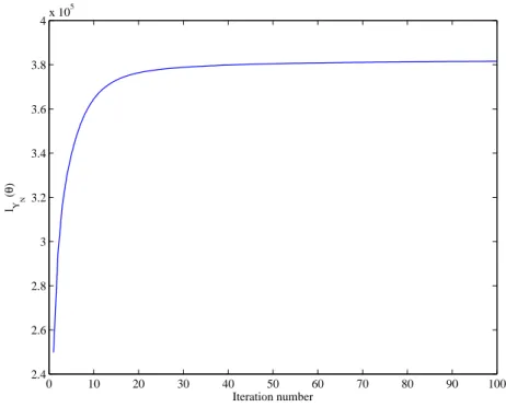
Hence, ignoring a constant, we may write the logarithm of the likelihood,LYN(θ), as:
lYN(θ) =logLYN(θ) = −
1 2
N X
k=1
log|Σk(θ)| −
1 2
N X
k=1
k(θ)0Σk(θ)−1k(θ) (19) 1Given the output data forstime stepsY
s={y1, y2, . . . , ys}is defined:
xsk =E[xk|Ys]
Pks
1,k2 =E
(xk1−x
s
k1)(xk2−x
s
k2)
T|Y
s
where it has been emphasized the dependence of the innovations on the parameters
θ. Of course, (19) is a highly nonlinear and complicated function of the unknown parameters. The usual procedure is to fix x0 and then develop a set or recursions for the log likelihood function and its first two derivatives. Then, a Newton-Raphson algorithm can be used successively to update the parameter values until likelihood is maximized.
0 10 20 30 40 50 60 70 80 90 100
2.4 2.6 2.8 3 3.2 3.4 3.6 3.8
4x 10 5
Iteration number
l YN
(
θ
)
Figure 1: LikelihoodLYN(θ)of a simulated case (it corresponds to case 1, numerical
example section)
In addition to Newton-Raphson, Shumway and Stoffer [3] presented a conceptually simpler estimation procedure based on the Expectation-Maximitation algorithm (EM). The EM algorithm is simple to apply since at each iteration the optimal solution for the unknown parameters can be obtained from explicit regression formulas.
The basic idea is that if we could observe the states XN = {x0, x1, x2, ..., xN},
in addition to the observations, YN = {y1, y2, . . . , yN}, then we could consider the
complete dataZN ={XN, YN}, with the joint density
f(ZN|θ) =fµ0,Σ0(x0)
N Y
k=1
fA,Q(xk|xk−1)
N Y
k=1
fC,R(yk|xk) (20)
where under the Gaussian assumption
fµ0,Σ0(x0) =
1 (2π)n/2|Σ
0|
1/2 exp{−
1
2(x0−µ0)
TΣ−1
fA,Q(xk|xk−1) =
1
(2π)n/2|Q|1/2 exp{−
1
2(xk−Axk−1)
TQ−1(x
k−Axk−1)} (22)
fC,R(yk|xk) =
1
(2π)l/2|R|1/2 exp{−
1
2(yk−Cxk)
T
R−1(yk−Cxk)} (23)
and the ”complete” data likelihood is defined byLXN,YN(θ) =f(ZN|θ).If we had the
complete dataZN, the maximum likelihood estimators (MLEs) ofθ would be easily
obtained fromLXN,YN(θ).The problem is more difficult than this, because we do not
know XN,and we have to estimate the parametersθfrom just the observed
informa-tionYN (the likelihood ofθgivenYN isLYN(θ)and it is related withLXN,YN(θ)).
The EM provides an iterative method for finding the MLEs of θ by succesively maximizing the conditional expectation of the complete likelihood LXN,YN(θ). The
log-likelihood lXN,YN(θ) = logLXN,YN(θ) is preferred because information can be
written as a sum of three uncoupled functions
lXN,YN(θ) =−
1
2[l1(µ0,Σ0) +l2(A, Q) +l3(C, R))]
where, ignoring constants
l1(µ0,Σ0) = log|Σ0|+ (x0−µ0)TΣ−01(x0−µ0) (24)
l2(A, Q) =Nlog|Q|+
N X
k=1
(xk−Axk−1)TQ−1(xk−Axk−1) (25)
l3(C, R) =Nlog|R|+
N X
k=1
(yk−Cxk)TR−1(yk−Cxk) (26)
Each iteration of the EM algorithm consists of two steps. Ifθj denotes the estimated
values of the parameterθ afterj iterations, the first step (E step) of the next iteration
j + 1is to compute
S(θ|YN, θj) = E[lXN,YN(θ)|YN, θj]. (27)
S(θ|YN, θj)is the key function of this method. The second step (M step) consists on
maximizing S(θ|YN, θj), what is equivalent to maximize the likelihoodLYN(θ) (see
fig. 1).
3.2.1 E-step: computation ofS(θ|YN, θj)
Note that given YN andθj the only terms that remain random (unknown) in (25) are
the states,xk. In this step, the algorithm compute the expected values of (25) respect to xk. Given the value of the parametersθfor iterationj, the Kalman filter and smoother
provides the following values fork= 0,1, . . . , N (see Appendix A):
xNk =E[xk|YN, θj] (28)
PkN =E[(xk−xNk)(xk−xNk) T|
Figure 2: Diagram of the analytical model of the benchmark structure
Pk,kN−1 =E[(xk−xkN)(xk−1−xNk−1)
T|
YN, θj] (30)
and from them it is possible to compute
E[l1(µ0,Σ0)|YN, θj] = log|Σ0|+tr
Σ−01P0N + (xN0 −µ0)(xN0 −µ0) (31)
E[l2(A, Q)|YN, θj] =Nlog|Q|+tr
Q−1Sxx−SxbAT −ASbx+ASbbAT (32) E[l3(C, R)|YN, , θj] =Nlog|R|+tr
R−1
Syy −SyxCT −CSxy +CSxxCT
(33) where
Sxx = N X
k=1
PkN +xNk (xNk )T (34)
Sxb= N X
k=1
Pk,kN−1+xNk(xNk−1)T) (35)
Sbb = N X
k=1
PkN−1+xNk−1(xNk−1)T) (36)
Syy = N X
k=1
ykykT
) (37)
Syx= N X
k=1
yk(xNk−1)T
) (38)
The functionS(θ|YN, θj)is the sum of the three terms of Equations (31)-(33), and
it depends on the parametersθ = (A, C, Q, R,µ0,Σ0). In the next section, the values
Base Floor 1 Floor 2 Floor 3 Floor 4
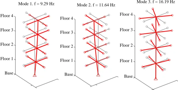
Mode 1. f = 9.29 Hz
Base Floor 1 Floor 2 Floor 3 Floor 4
Mode 2. f = 11.64 Hz
Base Floor 1 Floor 2 Floor 3 Floor 4
Mode 3. f = 16.19 Hz
Figure 3: First 3 eigenfrequencies and mode shapes computed from 12 DOF matrices (exact values)
3.2.2 M-Step: maximization ofS(θ|YN, θj)
Maximizing S(θ|YN, θj) with respect of the parameters θ, at iteration j, constitutes
the M-step and is analogous to the multivariate regression approach. This is the strong point of th EM algorithm, the maximum values are obtained from explicit formula.
The maximum ofE[l1(µ0,Σ0)|Yn, θj]is attained at
ˆ
µ0 =xN0 (39)
ˆ
Σ0 =P0N (40)
The estimation ofAcan be found equating to zero the derivative ofE[l2(A, Q)|YN, θj]:
ˆ
A=SxbSbb−1 (41)
and
ˆ
Q= 1
N
Sxx−SxbAˆT −ASˆ bx+ ˆASbbAˆT
(42)
In a similar way fromE[l3(C, R)|Yn, θj]the estimation ofCandRare:
ˆ
C=SyxSxx−1 (43)
ˆ
R= 1
N
Syy−SyxCˆT −CSˆ xy+ ˆCSxxCˆT
0 10 20 30 40 50 60 70 80 90 100 0
5 10 15 20
SSI method
frequency (Hz)
simulation
0 10 20 30 40 50 60 70 80 90 100
0 5 10 15 20
MLE + EM method
frequency (Hz)
simulation
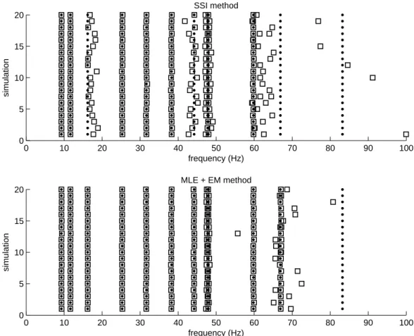
Figure 4: Eigenfrequency results corresponding to the first 20 simulated cases for the SSI and MLE+EM methods. The symbols “” and “” denote exact and estimated eigenfrequency, respectively.
3.2.3 Overall procedure
The overall method can be summarized as an iterative procedure as follows:
1. Initialize the procedure by selecting starting values for the parameters θ0 =
(A, C, Q, R,µ0,Σ0).
On iteration j (j = 1,2, . . .)
2. Compute the incomplete-data likelihood,LYN(θ
(j−1)).
3. Perform the E-Step. Use Properties A.1, A.2 y A.3 to obtain the smoothed valuesxNk, PkN, andPk,kN−1, fork = 1,2, . . . , N, using the parametersθ(j). Use the smoothed values to calculateSxb, Sbb, Sxx given in (34)-(36).
20 40 60 80 100 0.99
0.995 1 1.005 1.01
Mode1
SSI
20 40 60 80 100
0.99 0.995 1 1.005 1.01
Mode1
EM
20 40 60 80 100
0.99 0.995 1 1.005 1.01
Mode2
20 40 60 80 100
0.99 0.995 1 1.005 1.01
Mode2
20 40 60 80 100
0.99 0.995 1 1.005 1.01
Mode3
Simulation
20 40 60 80 100
0.99 0.995 1 1.005 1.01
Mode3
Simulation
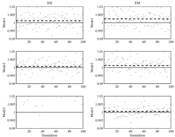
Figure 5: Eigenfrequency estimation results from 100 simulations. The estimates are divided by the true values (a value of 1 on the graphs indicates a perfect estimate). These relative frequencies are shown as dots. The scatter of this quantity gives an idea about the variance of the estimate. The average estimate is also shown (as a dashed line). The deviation of this quantity from 1 (full line) corresponds to the bias of the estimate. The rows show the modes; the columns represent the results of SSI and MLE+EM methods.
4
Numerical example
In this section, the effectiveness of the proposed identification method is evaluated via numerical simulations in the context of the ASCE benchmark problem for structural health monitoring.
4.1
Structural health monitoring benchmark problem
20 40 60 80 100 0
0.5 1 1.5 2
Mode1
SSI
20 40 60 80 100 0
0.5 1 1.5 2
Mode1
EM
20 40 60 80 100 0
0.5 1 1.5 2
Mode2
20 40 60 80 100 0
0.5 1 1.5 2
Mode2
20 40 60 80 100 0
0.5 1 1.5 2
Mode3
Simulation
20 40 60 80 100 0
0.5 1 1.5 2
Mode3
Simulation
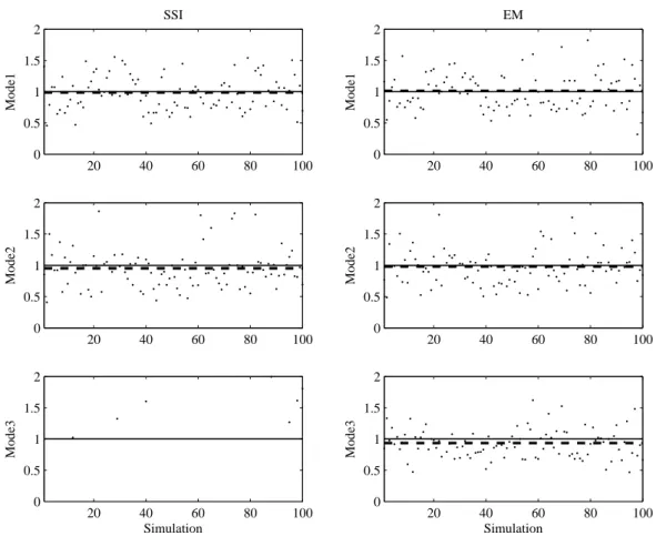
Figure 6: Damping ratio estimation results from 100 simulations. The estimates are divided by the true values (a value of 1 on the graphs indicates a perfect estimate). These relative damping ratios are shown as dots. The scatter of this quantity gives an idea about the variance of the estimate. The average estimate is also shown (as a dashed line). The deviation of this quantity from 1 (full line) corresponds to the bias of the estimate. The rows show the modes; the columns represent the results of SSI and MLE+EM methods.
of Engineering Mechanics contains the results of six different studies of the Phase I simulated benchmark problems, together with a definition and overview paper [7].
is shown in Fig. 2. The finite element models, by removing the stiffness of various elements, can simulate damage to the structure, and five damage patterns are defined for the structure. In this study has ben considered:
• 12 DOF undamaged structure.
• Classical damping (damping ratio equal to 0.01 for all modes).
• Sampling period is set as 0.001 s.
• Ten per cent root-mean-square (RMS) measurement noises.
The proposed method needs the following starting values (see Section 3.2.3):
• Starting values for the parameters θ0 = (A, C, Q, R,µ
0,Σ0). In this work
µ0 = 0, Σ0 = 0; the state space parameters identified using Stochastic Sys-tem Identification have been used as initial values forA, C, Q, R.
• 100 iterations for EM algorithm. Nevertheless, if
|LYN(θ
j+1)−L
YN(θ j)|
|LYN(θ
j)| <10
−10 (45)
the iteration loop is stopped (LYN is defined in Equation 19).
4.2
Discussion of results
Figure 3 shows the first three frequencies and mode shapes computed as the eigenval-ues and eigenvectors of M and K matrices. So these are exact results. On the other hand, it has been simulated 100 cases, and each simulated result consists in accelera-tions at 16 points of the structure. Figure 2 shows the location of these points: four at each floor, 2 in x-direction and 2 in y-direction.
A 24 order state space model has been identified from each simulated data set using SSI method and the proposed MLE+EM method. The estimated eigenfrequencies for the first 20 simulations are plotted in Figure 4. In a general sense, the proposed method identifies accurate eigenfrecuencies for modes 3, 7 and 11. Mode 12 are not identified by both methods.
20 40 60 80 100 0.96
0.98 1
Mode1
SSI
20 40 60 80 100
0.96 0.98 1
Mode1
EM
20 40 60 80 100
0.96 0.98 1
Mode2
20 40 60 80 100
0.96 0.98 1
Mode2
20 40 60 80 100
0.96 0.98 1
Mode3
Simulation
20 40 60 80 100
0.96 0.98 1
Mode3
Simulation
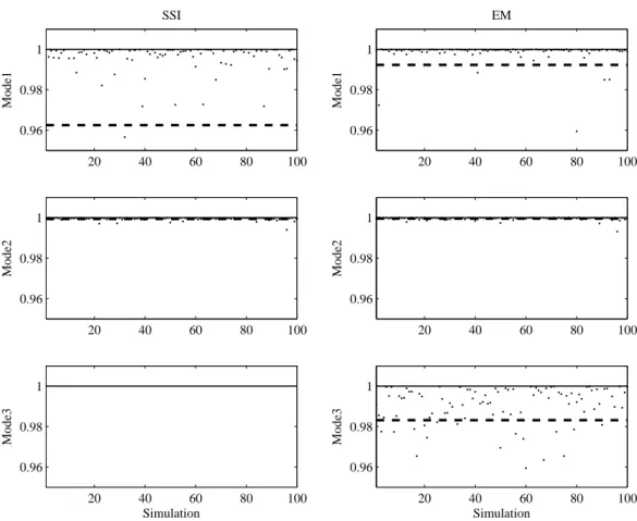
Figure 7: Mode shape estimation results from 100 simulations. The correlation be-tween the estimated and the true modes shapes are shown (as dots). The average of the estimates is also shown (as a dashed line). The rows show the modes; the columns represent the results of SSI and MLE+EM methods.
5
Conclusions
This paper presents a time-domain stochastic system identification method based on Maximum Likelihood Estimation (MLE) and Expectation Maximization (EM) algo-rithm. Advantages of the proposed structural identification method can be summa-rized as follows: (i) the method is based on maximum likelihood, that implies mini-mum variance estimates; (ii) EM is a computational simpler estimation procedure than other optimization algorithms; (iii) estimate more parameters than SSI, and this esti-mates are accurate. On the contrary, the main disadvantages of the method are two: (i) EM algorithm is an iterative procedure and it consumes time until convergence is reached; (ii) this method needs starting values for the parameters.
eigenfre-quencies, damping ratios and mode shapes reasonably well in the presence of 10% measurement noises even. These modal parameters are more acuratte than SSI esti-mated modal parameters.
References
[1] L. Ljung, ”System Identification. Theory for the users”. 2nd Ed., PTR Prentice-Hall, Upper Saddle River, N.J. 1999.
[2] P. Van Overschee, B. De Moor, ”Subspace Identification for Linear Systems. Theory - Implementation - Applications”. Kluwer Academic Publishers. 1996. [3] R.H. Shumway, D.S. Stoffer, ”Time series analysis and its applications”.
Springer. 2006.
[4] T. Katayama, ”Subspace Methods for System Identification”. Springer-Verlag London. 2005.
[5] M. Verhaegen, V. Verdult, ”Filtering and System Identification. A least squares approach”. Cambridge University Press. 2007.
[6] P. Van Overschee, B. De Moor. ”Subspace algorithm for the stochastic identifi-cation problem”, Automatica, 29, No. 3, 649-660. 1993.
[7] E. A. Johnson, H. F. Lam, L. S. Katafygiotis, J. L. Beck. ”Phase I IASC - ASCE structural health monitoring benchmark problem using simulated data.” J. Eng. Mech., 130(1), 315. 2004.
[8] IASC-ASCE SHM Task Group. Task group website (last visit on May 2010): http://bc029049.cityu.edu.hk/asce.shm/phase1/ascebenchmark.asp/
[9] B. Alicioglu, M. Lus, ”Ambient vibration analysis with subspace methods and automated mode selection: case studies”. Journal of Structural Engineering. ASCE. June 2008.
[10] B. Peeters, G. De Roeck, ”Stochastic System Identification for Operational Modal analysis: A Review”. Journal of Dynamic Systems, Measurement and Control. ASME. Vol. 123. December 2001.
Appendix
A
Kalman filter
Property A.1 (The Kalman Filter) For the state space model specified in (3) with initial conditionsx0
0 =µ0 andP00 = Σ0, fork= 1,2, . . . , N,
xkk−1 =Axkk−−11 (46)
Pkk−1 =APkk−−11AT +Q (47)
with
Pkk = [I −KkC]Pkk−1 (49)
where
Kk=Pkk−1CTΣ−k1 (50)
k=yk−E[yk|Yk−1] =yk−Cxkk1 (51)
Σk =var[C(xk−xkk−1+vk] =CPkk−1CT +R (52) Kkis called the Kalman gain andkare the innovations.
Property A.2 (The Kalman Smoother) For the state space model specified in (3) with initial conditionsxNN andPNN obtained via Property A.1, fork=N, N−1, . . . ,1,
xkN−1 =xkk−−11+Jk−1 xNk −x k−1
k
(53)
PkN−1 =Pkk−−11+Jk−1 PkN −Pk −1
k
JkT−1 (54)
where
Jk−1 =Pkk−−11A
T
Pkk−1−1 (55)
Property A.3 (The Lag-One Covariance Smoother) For the state space model spe-cified in(3), withKk,Jk(k= 1,2, . . . , N), andPNN obtained from Properties A.1 and
A.2, with initial condition
PN,NN −1 = (I−KNC)APNN−−11 (56) fork=N, N −1, . . . ,2
PkN−1.k−2 =Pkk−−11JkT−2+Jk−1 Pk,kN−1−AP
k−1
k−1
JkT−2 (57)