Uncertainty simulator to evaluate the electrical and mechanical deviations in
cylindrical near field antenna measurement systems
S. Burgos*, F. Martín, M. Sierra-Castañer, J.L. Besada
Grupo de Radiación, Dpto. Señales, Sistemas y Radiocomunicaciones,
Universidad Politécnica Madrid, 28040 Madrid, Spain
E-mail: [email protected]
Introduction
In order to evaluate how mechanical or electrical errors may affect in the final results (i.e.
radiation patterns, directivity, side lobe levels (SLL), beam width, maximum and null
position…), an error simulator based on virtual acquisitions of the measurement of the
radiation characteristics in a cylindrical near-field facility has been implemented [1], [2].
In this case, the Antenna Under Test (AUT) is modelled as an array of vertical dipoles
and the probe is assumed to be a corrugated horn antenna. This tool allows simulating an
acquisition containing mechanical errors – deterministic and random errors in the x-, y-
and z-position – and also electrical inaccuracies – such as phase errors or noise –. Then,
after a near-to-far-field transformation [3], by comparing the results obtained in the ideal
case and when including errors, the deviation produced can be estimated. As a result,
through virtual simulations, it is possible to determine if the measurement accuracy
requirements can be satisfied or not and the effect of the errors on the measurement
results can be checked. This paper describes the error simulator implemented and the
results achieved for some of the error sources considered for an L-band RADAR
antennas in a 15 meters cylindrical near field system.
Description of the error simulator for the inaccuracies evaluation
In this case, since the system where this work is applied is an outdoor system, there are
some error sources more relevant than the others. Actually, the effects of the wind for the
probe positioning and the temperature changes that affect the phase response of the
cables are the ones to be considered. Thus, the strategy adopted to evaluate the sources of
error is to simulate these deviations and to examine the influence that they have in the
final results. This procedure starts with the modelling of the transmitting and receiving
antennas. Then, the near-to-far-field transformation is applied to obtain the far-field
radiation patterns. So, to evaluate how errors could affect the final results, a model of the
antennas and a simulation of the acquisition process including errors has been performed.
Finally, the simulator compares the outcomes achieved from the reference data (i.e. the
array infinite far-field) with the ones including the deviations.
The received field in each point of the grid was calculated taking into account the
field radiated by all the dipoles modified by the probe pattern. The field from a dipole in
each point of the grid is given by the sum of three spherical waves [4]. The probe is an
ideal conical corrugated horn characterized by the calculated radiation pattern of the main
planes. For this investigation, the AUT evaluated is 5.3 meters long and 2.1 meters high.
In addition, the probe is modelled as an ideal horn (keeping
µ
=±1). Besides, the AUT
radiating elements considered are vertical
λ
/2 dipoles over a ground plane at a distance
equal to
λ
/4, and assumed to be infinite, so “Image Theory” can be applied. In addition, a
Error simulator for computational, mechanical and electrical errors
Computational errors
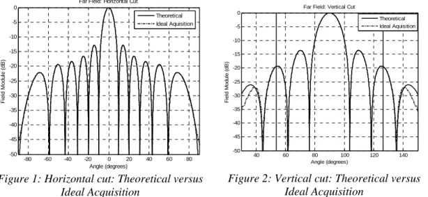
To validate the software and checking the computational errors of the algorithm, the array
infinite far-field of the antenna (product of factor array by the radiation element pattern)
is compared with the far-field calculated through the cylindrical near-field acquisition.
This tool was also useful for testing the elevation validity range of the near-to-far-field
transformation. The next figures show the results achieved:
-80 -60 -40 -20 0 20 40 60 80 -50
-45 -40 -35 -30 -25 -20 -15 -10 -5 0
Far Field: Horizontal Cut
Angle (degrees)
F
ie
ld
M
o
d
u
le
(
d
B
)
Theoretical Ideal Aquisition
Figure 1: Horizontal cut: Theoretical versus
Ideal Acquisition
40 60 80 100 120 140
-50 -45 -40 -35 -30 -25 -20 -15 -10 -5 0
Far Field: Vertical Cut
Angle (degrees)
F
ie
ld
M
o
d
u
le
(
d
B
)
Theoretical Ideal Aquisition
Figure 2: Vertical cut: Theoretical versus
Ideal Acquisition
The diagrams obtained showed a very good agreement between the theoretical far field
and the computed field and the validity of the angular margin of the measurement was
confirmed.
Pointing errors
There are two different sources of deterministic errors that affect the AUT pointing: the
axis non parallelism and the determination of the zero position of the azimuthal direction
(in this case, the random errors caused by the wind effect are not considered). Both
inaccuracies are directly translated to the error pointing, and they could be evaluated and
corrected to minimize them. While the axis non parallelism can be measured with an
optical procedure (i.e. laser tracker), the zero position of the azimuthal direction depends
on the RADAR positioner encoder and the triggering of the vector network analyzer that
can be either calculated or measured. Therefore, both errors can be compensated with a
rotation of the electric field [5], and as a result they are omitted for this study.
Mechanical errors in positioning system
The positioning errors in x- and y-direction can be very important because of the windy
outdoor conditions. To evaluate the effects of the mechanical errors on the outcomes,
some simulations were developed including systematic and random errors in each sample
in x, y and z directions. While the origin of the errors in x- and y-directions is the wind, in
the z direction is the mechanical system of the measurement tower. Besides, the
simulations were carried out with peak to peak error amplitudes in each sample from
±0.05
λ
to ± 0.2
λ
. From the diagrams acquired, it was clearly seen the noticeable
It is worthwhile noting that for the uniform random error in x-, y- and z-probe the
mean and standard deviation of the error introduced in the directivity were achievable.
From the results, it could be noticed that as expected the magnitude of the error in the
directivity increase while augmenting the error introduced in the acquisition process, as
shown in Figure 3 and Figure 4.
0.04 0.06 0.08 0.1 0.12 0.14 0.16 0.18 0.2 0.22 22 23 24 25 26 27
Directivity with and without error (dBi)
Error in Xprobe (random) [1/lambda]
D ir e c ti v it y ( d B i)
Dir without error Dir with error
Figure 3: Effect of a random error in the
X-position of the probe on the directivity
Mean and Standard Deviation of the Difference between the Directivity with and without Error 0,00 1,00 2,00 3,00 4,00 5,00
0,05 0,10 0,15 0,20
Error in Xprobe (random) [1/lambda]
M
e
a
n
Mean Error Difference Standard Deviation Error Difference
Figure 4: Mean and
σ
of the difference between the directivity with
and without random error in the X-position of the probe
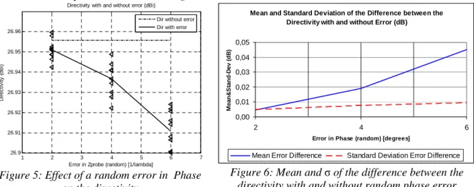
Phase errors
In near field antenna measurement systems the phase errors can be caused by temperature
variations during the acquisition process. The study carried out establishes the influence
that this inaccuracy may induce on the radiation pattern and directivity. As a
representative example of the results achieved, Figure 5 illustrates the effect of the
random phase error in the directivity when increasing the error magnitude. The line
shows the average values, the broken line the directivity without error and the triangles
show the result for each individual simulation. In this case, 10 iterations were carried out
for each of the peak to peak error amplitude. Since several simulations were performed
for each phase error, the mean and the standard deviations (
σ
) of the error in the
directivity were calculated, as Figure 6 shows.
1 2 3 4 5 6 7
26.9 26.91 26.92 26.93 26.94 26.95 26.96
Directivity with and without error (dBi)
Error in Zprobe (random) [1/lambda]
D ir e c ti v it y ( d B i)
Dir without error Dir with error
Figure 5: Effect of a random error in Phase
on the directivity
Mean and Standard Deviation of the Difference between the Directivity with and without Error (dB)
0,00 0,01 0,02 0,03 0,04 0,05
2 4 6
Error in Phase (random) [degrees]
M e a n & S ta n d -D e v ( d B )
Mean Error Difference Standard Deviation Error Difference
Figure 6: Mean and
σ
of the difference between the
directivity with and without random phase error
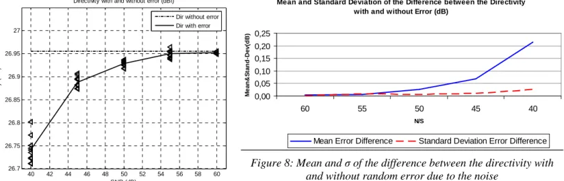
Errors due to the dynamic range
Regarding the Signal to Noise Ratio (SNR) in the receiver, this magnitude can be
evaluated for considering its influence on the side lobe levels. This effect was
accomplished adding a white Gaussian noise to each value of the acquired field with
respect to the maximum. Figure 7 and Figure 8 represent the results achieved:
40 42 44 46 48 50 52 54 56 58 60 26.7
26.75 26.8 26.85 26.9 26.95 27
Directivity with and without error (dBi)
SNR (dB)
D
ir
e
c
ti
v
it
y
(
d
B
i)
Dir without error Dir with error
Figure 7: Effect of the noise on the directivity
Mean and Standard Deviation of the Difference between the Directivity with and without Error (dB)
0,00 0,05 0,10 0,15 0,20 0,25
60 55 50 45 40
N/S
M
e
a
n
&
S
ta
n
d
-D
e
v
(d
B
)
Mean Error Difference Standard Deviation Error Difference