Mathematical Interpolation Methods for Spatial Estimation of
Global Horizontal Irradiation in Castilla-León, Spain: a case
study
M. C. Rodríguez-Amigo (1), M. Díez-Mediavilla (1), D. González-Peña (1), A. Pérez-Burgos (1,2), C. Alonso-Tristán (1, *)
(1) Research Group SWIFT (Solar and Wind Feasibility Technologies). Escuela Politécnica Superior (E.P.S) Universidad de Burgos. Spain.
(2) Dpto Física Aplicada. Facultad de Ciencias. Universidad de Valladolid, Spain. (*) Corresponding author: [email protected]; [email protected] Abstract:
Four spatial interpolation methods (Inverse Distance Weighted, Spline, Kriging and
Natural Neighbor) and their different variations are employed to map Global Horizontal
Irradiation (GHI) in Castilla-León, Spain. The work has been performed using the software
ArcGis, widely used in geostatistical applications, showing the versatility of the system
and its applicability to climate data. The measuring network consists of 71 ground
meteorological stations that use seven complete years of half-hourly data sets, yielding
annual daily averages of GHI. The interpolation results are tested against data from the four
Spanish National Meteorological Agency (AEMET) stations available in the region using
standard statistical indicators (RMSE, MBE, MAPE and MAE). An additional partial cross
validation of the results, which excludes five stations from the measuring network, employs
different criteria to verify the results of the interpolation methods applied. This work
contributes to the classification of interpolation methods to obtain climatological data
across large areas with a low number of irregularly distributed of measurement points and
with a low topographic complexity. The Universal Kriging method with quadratic
semi-variogram shows the best results taking into account the RMSE and MAE statistical
indicators.
Keywords:
1. Introduction
Solar radiation is the major available renewable energy source. Solar radiation prediction
and forecasting are important for electricity generation and use of alternative energy
sources on line. The availability of solar radiation measurements at any given location
would give valuable information for the realization of energy projects. This form of
resource monitoring is, therefore, critical for system design and assessment, energetic
planning, and grid management. A key objective for successful network monitoring is to
map relevant parameters and predict their values at unobserved locations, by employing
their values at known locations. In the case of solar energy, Global Horizontal Irradiation
(GHI) is the most common parameter recorded by meteorological ground stations. Even
though their accuracy is restricted, several mathematical methods to obtain values of GHI
through the use of different meteorological data, such as temperature, rainfall, and
geographical parameters, have been proposed (Ayodele and Ogunjuyigbe, 2015; Chelbi et
al., 2015; Dumas et al., 2015; Kim et al., 2014; Mousavi et al., 2015; Sun et al., 2015; Wu
et al., 2013). In other hand, satellite based maps a reliable technique widely accepted and
several commercial products are available from this technique (Perez et al., 1994). But the
ground measurements are essential to test any method to calculate the solar resource. As
the number of ground stations is limited, limiting the availability of data, mathematical
interpolation methods can provide suitable results, without the need to establish additional
meteorological parameters.
In this work, four main interpolation methods and 29 variations were used to map annual
daily average values of GHI (MJ m-2 day-1) from a network of 71 ground stations in
Castilla-León, Spain. The four AEMET (National Meteorological Agency) facilities in the
region constitute the control system. Standard statistical indicators are used to classify the
interpolation mathematical methods for solar radiation data over large areas with few
measuring points. The work has been performed using the ArcGis Software, which is
widely used in geostatistical applications, showing the versatility of the system and its
applicability to climate data.
The work is organised as follows: The region under study and its climatic characteristic are
described in Section 2; both ground meteorological networks, SIAR and AEMET, used for
the application of the interpolation methods and their validation are described in the Section
3. In Section 4 a wide review of the main interpolation methods traditionally used for
climatic data is presented. The obtained results from the application of the interpolation
methods on the basis of the classical statistical indicators are presented and discussed in
Section 5. Finally, the main conclusions and contributions of the paper are detailed in
Section 6.
2. The region under study
Castilla-León is a Spanish region located in the northern half of the central Meseta, an
extensive plateau with a very low population density (27 habitants/km2) that occupies a
surface area of 94226 km2. Surrounded by mountain ranges, with heights in the range
between 700 and 1000 m above sea level. The continental Mediterranean climate of
Castilla-León has long, cold winters with average ambient temperatures between 4ºC and
7ºC in January and short, dry and hot summers, with ambient temperatures between 19ºC
and 22ºC. Scant rainfall is accentuated in lower areas, as the higher mountainous areas act
as natural barriers, interrupting cloud formation and causing uneven patterns of
precipitation.
Three different climatic areas may be identified: a) to the north, at the highest part of the
elevations, typical Atlantic climates prevail with very cold winters; b) the central area of
the plateau is dominated by a Continental Mediterranean climate with hot summers and
severe winters, except to the east of the province of Zamora, where the climate is much
drier. c) A typical mountainous Mediterranean climate prevails in the highly elevated areas
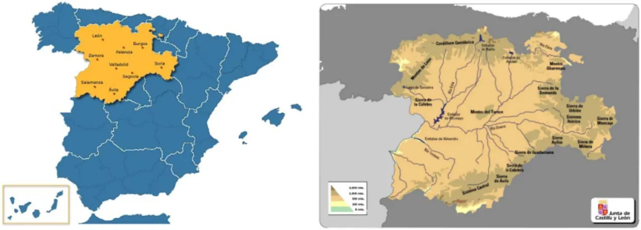
of the north-east, east and south, with hot summers, cold winters and low rainfall. Figure 1
shows the geographical location of Castilla-León.
Figure 1. a) Location of Castilla-León, Spain; b) River Duero flowing across the region from East to West (Source: http://navalmanzano.com/ ; http://mapasinteractivos.didactalia.net/
Among the geophysical and climatic features described above, the height above sea level
of Castilla-León, above that of its surrounding regions, may be the most influential factor
in the solar radiation that it receives. The geographical coordinates (40º05’ longitude and
43º14’ latitude) mean that the diurnal duration between winter (slightly less than nine
hours) and summer (over 15 hours) is markedly different, a fact that implies much higher
levels of irradiance in summer than in winter.
3. Experimental Section 3.1. SIAR network
SIAR (Sistema de Información Agroalimentaria para el Regadío, Agricultural Information
System for Irrigation) (Ministerio de Agricultura) is a ground meteorological network
Castilla-León, the SIAR System has 53 ground stations, which collect data on GHI,
temperature, rainfall, humidity, wind speed and wind direction. The locations of each
station comply with the directives of both the World Meteorological Organization (WMO)
(World Meteorological Organization, 2012) and AEMET (Agencia Estatal de
Meteorología). A Skye SP1110 pyranometer (spectral range 350-1100 nm, uncertainty
±5%), calibrated in accordance with ISO 9847, is used to measure GHI with a sampling
rate of 10 seconds. Half-hourly data are logged by a SR1000 Campbell datalogger. A strict
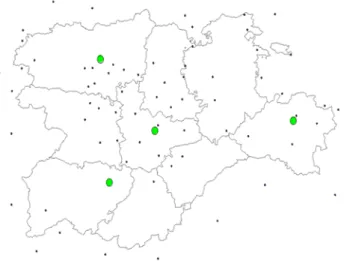
filtering procedure has been applied to the available data and the number of ground stations
supplying data for the study has been limited to 44 (see Figure 2). This meteorological
network has been amply used to test different methodologies to obtain solar irradiation
maps by using support vector machines (Antonanzas-Torres et al., 2015; Antonanzas et al.,
2015), satellite data (Antonanzas-Torres et al., 2013a) or parametric (Antonanzas-Torres
et al., 2013b) and predictive models (Urraca et al., 2016).
3.2.The boundary area
The SIAR network has few ground stations along the borders of the Region, so a set of
ground station in the neighboring regions were used to mitigate abrupt responses in the
interpolation method. The search to find ground stations in the boundaries with similar
technical characteristics and data over the same time period was, therefore, extended to the
regions of Galicia, Asturias, Cantabria, País Vasco, La Rioja, Aragón, Castilla La Mancha,
Madrid, Extremadura and Portugal.
3.3. The control network: AEMET ground stations
The AEMET stations located in Castilla-León were reserved as the validation sites, and
were not used for the interpolation methods. Only four stations in the AEMET network
record GHI data in Castilla-León. Kipp&Zonen CM11 or CM21 pyranometers (spectral
hourly GHI values were calculated using the integration trapezoidal rules over the 10
seconds values. A partial cross-validation of the results in accordance with different criteria
was also performed using five additional controls; each consisting of five stations
(approximately 10% of the total SIAR network) in the interpolation network.
3.4. Data processing
Data sets from 2007 to 2013 (seven complete years) were compiled for the study. Data
available from the SIAR meteorological network were stored on a database and validated
in accordance with UNE 500540-2004 (Guidance for the validation of weather data from
station networks). Moreover, the data were checked against the WMO criteria as a
safeguard against faulty data. Further quality criteria secured that only the stations that had
logged at least five complete years, with no less than 335 data sets per year, were
considered for the study. In summary, sixty-seven ground stations were used for this study:
44 of them from Castilla-León and 27 located outside the Region but close to its borders.
Figure 2 shows the distribution of all ground stations that gave 110080 daily GHI values
used in the study. Cumulative daily GHI values were calculated using the integration
trapezoidal rules over the half-hourly values of the database.
Different interpolation methods implemented in ArcGis-10 Software were applied to the
data: Inverse Distance Weighted (IDW), Natural Neighbor, Spline and Kriging. 29 variants
of these methods were used, changing different parameters as the number of interpolation
points, weight or power. The four conventional statistical indicators in use, RMSE, MBE,
MAE and MAPE (%), are defined as follows:
∑
% (Eq. 1)
∑ % (Eq. 2)
∑| | % (Eq. 3.)
∑ 100 (Eq. 4)
where, is the experimental value and is the calculated one. These statistical
indicators are representative values of the quality of the interpolation method used to fit the data
4. Interpolation methods for climatic and meteorological data
Interpolation methods have traditionally been applied to geospatial data, based on Tobler’s
first law of geography: “Everything is related to everything else, but near things are more
related than distant things” (Tobler, 1979). Franke (Franke, 1982), and Lam (Lam, 1983)
reviewed and classified various interpolation techniques. A complete report about
interpolation techniques for Solar Radiation data was published by IEA (International
Energy Agency) (Zelenka et al., 1992). The main novelty of the present work is the use of
ArcGis 10 Software that implements the interpolation methods and maps the results. A
viewable rectangular (raster map) pixel grid of the working area was built by applying the
mathematical interpolation methods to the interpolation network. Several methods were
implemented in the software. The use of ArcGIS allows the modification of the different
available data. The results can be presented in the form of maps onto the studied area. The
main characteristics of these methods are summarized below.
4.1 Inverse Distance Weighting (IDW)
The simplest spatial interpolation method is the IDW (Inverse Distance Weighting)
method, consisting of weighting the inverse of the distance between two points in the
sample. The influence of the proximity between data can be defined in a deterministic or
an analytical way (Gutierrez-Corea et al., 2014). This method has been used successfully
to obtain climatic parameters, (Apaydin et al., 2004; Güler, 2014; Wu et al., 2013).
Antonanzas et al (Antonanzas et al., 2015) indicated that IDW is a suitable method to
estimate GHI in areas where a low number of solar stations is available.
The fundamental parameter of the method is the power, assigned to calculate the influence
of the known values (interpolation network) to the calculated values depending on the
distance between them. Power is a real positive number that controls the influence of the
nearest points obtaining softer surfaces when the power is fixed to 2. An optimization
engine is available in ArcGis to fix this parameter. All interpolated points must tie within
the range of the data and if peaks and troughs are not specifically sampled, they cannot be
inferred.(Watson and Philip, 1985)..
4.2. Kriging method
Kriging is the other standard interpolation procedure. The interpolated values are modeled
by a Gaussian process governed by a previous co-variance estimation method. This method
uses a variogram model for data collection, calculating the weights given to each point used
in the valuation of the references. This interpolation technique is based on the premise that
spatial variation continues in the same tendency. Different weighting calculation
the various degrees of assumed stationarity. Universal Kriging (UK) assumes a structural
component in the series of values, which implies a local variable trend. In Ordinary Kriging
(OK), local averages are not necessarily close to the population mean, so that neighboring
points are hardly used for estimation. The available variogram models are linear and
quadratic for UK and circular, spherical, exponential, Gaussian and linear for OK.
The Kriging method can provide suitable results for GHI values in homogenous places,
with similar climatic parameters. But height, orientation and possible shadows caused by
the specific topographical variations in complex topographic areas could negatively
influence the results, making them less reliable. Different Kriging methods have been used
in this way by Alsamamra et al. (Alsamamra et al., 2009) introducing other external
variables to include additional information to improve the results, or to complete unknown
values in a database of continuous data (Goovaerts, 2000; Jeffrey et al., 2001; Kambezidis
et al., 2016).The Kriging method reduces significantly the errors when more points are
used in the interpolation network (Antonanzas et al., 2015)
4.3. Natural Neighbor
Values that are closer to the search point are used as input data for the natural neighbor
interpolation. The weighting of each point is based on proportional areas. This method is
known as Sibson’s interpolation (Sibson, 1981). The natural neighbors of a point are those
associated with adjacent Thiessen polygons. A Voronoi’s diagram with all of the
interpolation data is built around the search point as well as the new polygons. The overlap
between both areas is assumed as the weighting.
4.4. Splines
A spline is a piecewise differential function defined through low-degree polynomial
surface containing all the input data. Intervals are needed to avoid abrupt changes in large
surfaces. A complete mathematical formalism was developed by Wahba et al. (Wahba and
Wendelberger, 1980) modifying Sasaki’s approach (Sasaki et al., 1960)
The values are estimated using a mathematical function that minimizes the general
curvature of the surface for obtaining a smooth surface that contains all the input data. Two
additional parameters are needed to control the output: the weighting and the number of
points. The weight reflects the contribution to the results of the third derivatives of the
function. The output surface is smoother at higher weighting values. The number of points
used for the interpolation has some influence on the shape of the surface, but increases the
computation time.
5. Results and Discussion
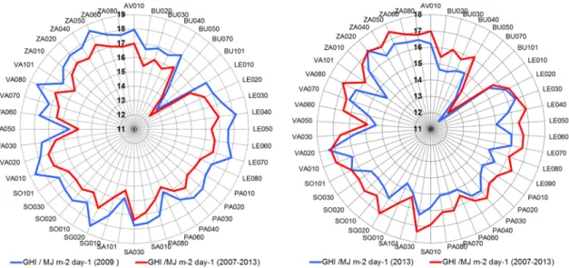
A preliminary analysis of the results using 46 stations of the SIAR network was carried out
to establish the distribution of the irradiation across the studied area. Average daily GHI
(MJ m-2day-1) was calculated for the 46 stations of the SIAR network chosen for the study
using the available data of the 7-year period. Values of maximum, minimum and average
daily GHI were calculated for all stations and years. Significant differences between the
stations were found, as shown in Figure 3. Comparisons between the seven year GHI
average and the GHI average for a single year average reflected important differences, as
can be seen in Figure 3: 2009 was above average and 2013 below average for the complete
network. As an initial result, the number and the particular characteristic of the years
considered for the study have a very significant influence on the results. Therefore, very
Figure 3: Comparison of daily annual average of GHI (MJ m-2 day-1) calculated using 1-year data (2009 or 2013) and 7-year data (2007-2013)
Maps of the annual daily GHI average (MJm-2 day-1) in Castilla-León were calculated using
the following interpolation methods and their different variations: IDW, Natural Neighbor,
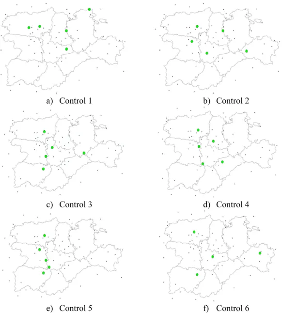
Kriging and Splines. A partial-cross validation was performed: five controls were
established using the 5 stations in the control system (10% of the total) and 66 stations in
the interpolation network. In each control (1 - 5), interpolated values were compared to
those measured at the validation sites using the previously defined standard statistical
indicators. Different criteria were used to select the stations for each control: longitude and
latitude of the stations, proximity between them, and proximity to the border area, as well
as proximity between the validation sites and the interpolation network stations. Figure 4
shows the distribution of the stations used in each control in the Region. Definitive control
a) Control 1 b) Control 2
c) Control 3 d) Control 4
e) Control 5 f) Control 6
Figure 4: Distribution of the stations chosen for each control system following different criteria : a) Control 1: Stations located in the North of the Region under study including a station at the border; b) Control 2: Stations at some distance from each other that cover the most extensive area and include at least
one station per province; c) Control 3: Stations at some distance from each other which cover the largest possible area and include an isolated station; d) Control 4: Stations centered in the area under study; e)
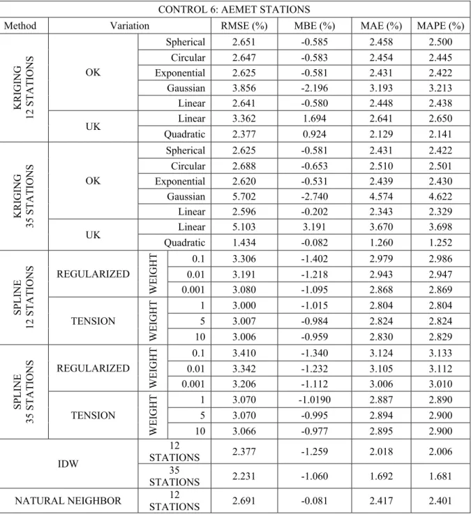
Control 5: Stations on a similar longitude; f) Control 6: Definitive control system using the AEMET stations in the Region.
All the methods yielded RMSE values below 6%; the use of different control systems
(controls 1 to 5) added no significant differences. Using stations belonging to the SIAR
network as the control stations, the OK method with 35 stations and quadratic
and the quadratic semivariogram showed the lowest MAE value. In Table 1, the results of
the interpolation methods and variations, using the AEMET control system stations, are
shown. The previously defined statistical parameters -RMSE (%), MBE (%), MAE(%) and
MAPE(%)- are included. All these methods presented RMSE (%) values lower than 4%.
Table 1: Standard Statistical indicators (%) of the results of the different spatial interpolation methods applied to the SIAR network in Castilla-León. Control implemented by the four AEMET stations located in
The interpolation methods underestimate GHI, as show the negative values of MBE. “The
interpolation method that gave the lowest RMSE value (1.4 %), significantly lower than
the other analyzed methods, was UK-35 stations, quadratic semi variogram. The other
statistical indicators calculated, MBE, MAE and MAPE, show also the lowest values for
the same case. This method was considered the best for this Region and data series. Figure
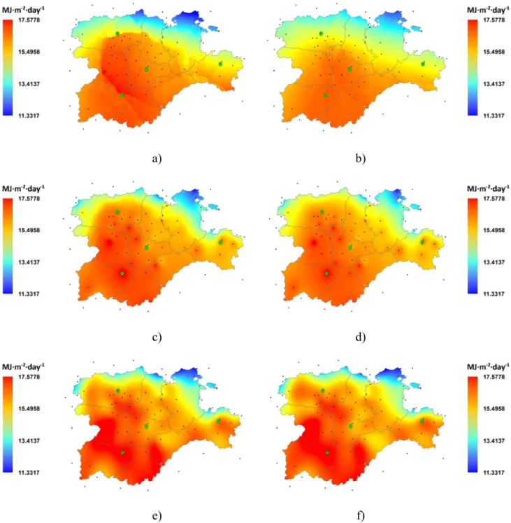
5 shows the annual daily average of GHI maps in Castilla-León calculated by different
interpolation methods. Figure 5-a shows the results using the UK interpolation method and
the linear semivariogram (12 stations) and Figure 5-b the UK-linear method (35 stations),
which influences the grid resolution. Similar results are shown in Figures 5-c and 5-d for
the IDW interpolation method and in Figures 5-e and 5-f for the Regularized Spline (RS).
Numerical indicators of these figures are shown in Table 1. As can be seen, the resolution
of the grid (number of interpolation points) is not related to the performance of the method:
UK and RS yielded the most promising results using a 12-point interpolation rather than a
35-point interpolation, in opposition to the IDW method, which presented better results
a) b)
c) d)
e) f)
Figure 5: Maps of daily average of GHI (MJ m-2 day-1) obtained through different interpolation methods and variations of them; a) UK-linear-12; b) UK linear-35; c) IDW-12; d) IDW-35; e) Regularized Spline,
12 points, weight 0.01; f) Regularized Spline, 35 points, weight 0.01
6. Conclusions
Conventional interpolation methods for climatic and meteorological data have been
reviewed and applied to build global horizontal irradiation maps in Castilla-León, Spain.
meteorological network used for this work. The SIAR network in the area under study has
been complemented by similar ground stations in the boundary area to avoid abrupt
responses of the interpolation methods. The interpolation network was, therefore, consisted
of 71 stations: 44 in Castilla-León and 27 in the boundary area. Seven complete years of
half-hourly GHI data have been used to calculate daily GHI and to obtain annual averages.
Significant differences have been found in the seven-year data series, a result that
highlights the decisive nature of the temporal series in the results.
An important difference in the annual daily average value of GHI has been observed across
the Region from east to west, with a maximum difference of 12.7% across 250 km. This
difference had a significant impact on the electrical production at PV facilities, which can
be estimated at 7200 €/year for a typical 100 kW facility under current Spanish Legislation.
GHI values were estimated in the range 14-18 MJm-2 day-1, equivalent to 4 kWh/day or
1460 kWh/year per installed kW. This variation could be explained by the geographical
characteristic of the Region with an extensive plain to the west that is not conducive to the
accumulation of cloud cover.
The work has been performed using the ArcGis-10 Software, widely used in geoestatistical
applications. This system allows an easy implementation of the different interpolation
methods, modifying the parameters necessary to perform a complete study of the available
data.
On the basis of the individual goodness of each interpolation method in this investigation,
the application of Ordinary Kriging with Gaussian semi-variograms to the area under study
has been rejected. This method always obtained the highest deviation from the
experimental results (regardless of the controls in use). The number of interpolation points
area under study was UK-35 points and quadratic semi-variogram taking the RMSE and
MAE results into account.
A more homogeneous distribution of the stations in the interpolation network would be
advisable, to improve the results of this study. As Figure 2 shows, there is an accumulation
of ground stations in the center of the region but large empty areas around the boundaries.
In this sense, this work shows that the interpolation methods are a suitable procedure to
obtain climatological data across large areas with a low number of irregularly distributed
of measurement points and with a low topographic complexity.
7. Acknowledgments
This research received economic support from the Spanish Government (Grant
ENE2014-54601-R) and Junta de Castilla-León (BU034U16). One of the authors, David González
Peña, thanks to Junta de Castilla-León and European Social Fund (Orden EDU/310/2015)
for financial support.
8. References
Alsamamra, H., Ruiz-Arias, J.A., Pozo-Vázquez, D., Tovar-Pescador, J., 2009. A
comparative study of ordinary and residual kriging techniques for mapping global solar
radiation over southern Spain. Agric. For. Meterol. 149, 1343-1357.
Antonanzas-Torres, F., Cañizares, F., Perpiñán, O., 2013a. Comparative assessment of
global irradiation from a satellite estimate model (CM SAF) and on-ground measurements
(SIAR): A Spanish case study. Renewable and Sustainable Energy Reviews 21, 248-261.
Antonanzas-Torres, F., Sanz-Garcia, A., Martínez-de-Pisón, F.J., Perpiñán-Lamigueiro,
O., 2013b. Evaluation and improvement of empirical models of global solar irradiation:
Antonanzas-Torres, F., Urraca, R., Antonanzas, J., Fernandez-Ceniceros, J.,
Martinez-De-Pison, F.J., 2015. Generation of daily global solar irradiation with support vector machines
for regression. Energy Convers Manage 96, 277-286.
Antonanzas, J., Urraca, R., Martinez-De-Pison, F.J., Antonanzas-Torres, F., 2015. Solar
irradiation mapping with exogenous data from support vector regression machines
estimations. Energy Convers Manage 100, 380-390.
Apaydin, H., Kemal Sonmez, F., Yildirim, Y.E., 2004. Spatial interpolation techniques for
climate data in the GAP region in Turkey. Clim. Res. 28, 31-40.
Ayodele, T.R., Ogunjuyigbe, A.S.O., 2015. Prediction of monthly average global solar
radiation based on statistical distribution of clearness index. Energy 90, Part 2, 1733-1742.
Chelbi, M., Gagnon, Y., Waewsak, J., 2015. Solar radiation mapping using sunshine
duration-based models and interpolation techniques: Application to Tunisia. Energy
Conversion and Management 101, 203-215.
Dumas, A., Andrisani, A., Bonnici, M., Graditi, G., Leanza, G., Madonia, M., Trancossi,
M., 2015. A new correlation between global solar energy radiation and daily temperature
variations. Solar Energy 116, 117-124.
Franke, R., 1982. Scattered data interpolation: Tests of some methods. Mathematics of
computation 38, 181-200.
Goovaerts, P., 2000. Geostatistical approaches for incorporating elevation into the spatial
interpolation of rainfall. J. Hydrol. 228, 113-129.
Güler, M., 2014. A comparison of different interpolation methods using the geographical
information system for the production of reference evapotranspiration maps in Turkey. J.
Gutierrez-Corea, F.V., Manso-Callejo, M.A., Moreno-Regidor, M.P., Velasco-Gómez, J.,
2014. Spatial estimation of sub-hour global horizontal irradiance based on official
observations and remote sensors. Sensors 14, 6758-6787.
Jeffrey, S.J., Carter, J.O., Moodie, K.B., Beswick, A.R., 2001. Using spatial interpolation
to construct a comprehensive archive of Australian climate data. Environ. Model. Softw.
16, 309-330.
Kambezidis, H.D., Psiloglou, B.E., Kavadias, K.A., Paliatsos, A.G., Bartzokas, A., 2016.
Development of a Greek solar map based on solar model estimations. Space Research and
Technologies Institute Bulgarian Academy of Sciences, 57.
Kim, K.H., Baltazar, J.-C., Haberl, J.S., 2014. Evaluation of Meteorological Base Models
for Estimating Hourly Global Solar Radiation in Texas. Energy Procedia 57, 1189-1198.
Lam, N.S.-N., 1983. Spatial interpolation methods: a review. The American Cartographer
10, 129-150.
Ministerio de Agricultura. SIAR: Sistema de Información Agroclimática para el Regadío.
Available in: http://www.mapa.es/siar/Informacion.asp Last accessed: (May, 2017)
Mousavi, S.M., Mostafavi, E.S., Jaafari, A., Jaafari, A., Hosseinpour, F., 2015. Using
measured daily meteorological parameters to predict daily solar radiation. Measurement
76, 148-155.
Perez, R., Seals, R., Stewart, R., Zelenka, A., Estrada-Cajigal, V., 1994. Using
satellite-derived insolation data for the site/time specific simulation of solar energy systems. Sol.
Energy 53, 491-495.
Sasaki, Y., Texas, A., System, M.U., Department of, O., Meteorology, 1960. An objective
analysis for determining initial conditions for the primitive equations. Texas A & M
Sibson, R., 1981. A brief description of natural neighbour interpolation. Interpreting
multivariate data 21, 21-36.
Sun, H., Zhao, N., Zeng, X., Yan, D., 2015. Study of solar radiation prediction and
modeling of relationships between solar radiation and meteorological variables. Energy
Conversion and Management 105, 880-890.
Tobler, W.R., 1979. Smooth pycnophylactic interpolation for geographical regions. Journal
of the American Statistical Association 74, 519-530.
Urraca, R., Antonanzas, J., Alia-Martinez, M., Martinez-De-Pison, F.J.,
Antonanzas-Torres, F., 2016. Smart baseline models for solar irradiation forecasting. Energy Convers
Manage 108, 539-548.
Wahba, G., Wendelberger, J., 1980. Some new mathematical methods for variational
objective analysis using splines and cross validation. Monthly weather review 108,
1122-1143.
Watson, D., Philip, G., 1985. Comment on “a nonlinear empirical prescription for
simultaneously interpolating and smoothing contours over an irregular grid” by F. Duggan.
Computer methods in applied mechanics and engineering 50, 195-198.
World Meteorological Organization, 2012. Guide to meteorological instruments and
methods of observation. Secretariat of the World Meteorological Organization.
Wu, W., Tang, X.P., Yang, C., Guo, N.J., Liu, H.B., 2013. Spatial estimation of monthly
mean daily sunshine hours and solar radiation across mainland China. Renew. Energy 57,
546-553.
Zelenka, A., Czeplak, G., D'Agostino, V., 1992. Techniques for Supplementing Solar