Modelling laser milling of microcavities for the manufacturing of DES with ensembles

(1)

Research Article

Modelling Laser Milling of Microcavities for

the Manufacturing of DES with Ensembles

Pedro Santos,

1

Daniel Teixidor,

2

Jesus Maudes,

1

and Joaquim Ciurana

2

1_{Department of Civil Engineering, Higher Polytechnic School, University of Burgos, Cantabria Avenue, 09006 Burgos, Spain} 2_{Department of Mechanical Engineering and Industrial Construction, University of Girona, Maria Aurelia Capmany 61,}

17003 Girona, Spain

Correspondence should be addressed to Jesus Maudes; [email protected]

Received 28 December 2013; Accepted 11 March 2014; Published 17 April 2014

Academic Editor: Aderemi Oluyinka Adewumi

Copyright © 2014 Pedro Santos et al. This is an open access article distributed under the Creative Commons Attribution License, which permits unrestricted use, distribution, and reproduction in any medium, provided the original work is properly cited.

A set of designed experiments, involving the use of a pulsed Nd:YAG laser system milling 316L Stainless Steel, serve to study the laser-milling process of microcavities in the manufacture of drug-eluting stents (DES). Diameter, depth, and volume error are considered to be optimized as functions of the process parameters, which include laser intensity, pulse frequency, and scanning speed. Two different DES shapes are studied that combine semispheres and cylinders. Process inputs and outputs are defined by considering the process parameters that can be changed under industrial conditions and the industrial requirements of this manufacturing process. In total, 162 different conditions are tested in a process that is modeled with the following state-of-the-art data-mining regression techniques: Support Vector Regression, Ensembles, Artificial Neural Networks, Linear Regression, and Nearest Neighbor Regression. Ensemble regression emerged as the most suitable technique for studying this industrial problem. Specifically, Iterated Bagging ensembles with unpruned model trees outperformed the other methods in the tests. This method can predict the geometrical dimensions of the machined microcavities with relative errors related to the main average value in the range of 3 to 23%, which are considered very accurate predictions, in view of the characteristics of this innovative industrial task.

1. Introduction

Laser-milling technology has become a viable alternative to conventional methods for producing complex microfeatures on difficult-to-process materials. It is increasingly employed

in the industry, because of its established advantages [1].

As a noncontact material-removal process, laser machining removes smaller and more precise amounts of material, applies highly localized heat inputs to the workpiece, min-imizes distortion, involves no tool wear, and is not subject to certain constraints such as maximum tool force, buildup edge formation, and tool chatter. Micromanufacturing pro-cesses in the field of electronics and medical and biological applications are a growing area of research. High-resolution components, high precision, and small feature size are needed in this field, as well as real 3D fabrication. Thus, the use of laser machining to produce medical applications has become a growing area of research, one example of which

is the fabrication of coronary stents. This research looks at the fabrication and performance of the DES. Some of these DES are metallic stents that include reservoirs that

contain the polymer and the drug [2], such as the Janus

TES stent [3] which incorporates microreservoirs cut into its

abluminal side that are loaded with the drug. The selection of the laser system and the process parameters significantly affects the quality of the microfeature that is milled and the productivity of the process. Although there are several studies which deal with the effect of the process parameters on the quality of the final laser-milled parts, few of them study this effect on a microscale. The literature contains many examples of experimental research looking at the influence of scanning speed, pulse intensity, and pulse frequency on the quality and productivity of laser milling in different

materials on a macroscale [4–7]. There are many works on

microscale machining that have investigated laser-machining

processes in laser microdrilling [8–10], laser microcutting

(2)

[11–13], and laser micromilling in 2D [14,15]. However, there is little research on laser 3D micromilling. Pfeiffer et al.

[16] studied the effects of laser-process parameters on the

ablation behaviour of tungsten carbide hard metal and steel using a femtosecond laser for the generation of complex 3D

microstructures. Karnakis et al. [17] demonstrated the

laser-milling capacity of a picoseconds laser in different materials (stainless steel, alumina, and fused silica). Surface topology information was correlated with incident power density, in

order to identify optimum processing. Qi and Lai [18] used a

fiber laser to machine complex shapes. They developed a ther-mal ablation model to determine the ablated material volume and the dimensions and optimized the parameters to achieve maximum efficiency and minimum thermal effects. Finally,

Teixidor et al. [19] studied the effects of scanning speed, pulse

intensity, and pulse frequency on target width and depth dimensions and surface roughness for the laser milling of microchannels on tool steel. They presented a second-order model and a multiobjective process optimization to predict the responses and to find the optimum combinations of process parameters.

Although the manufacturing industry is interested in laser micromilling and some research has been done to understand the main physical and industrial parameters that define the performance of this process, the conclusions show that analytical approaches are necessary for all real cases due to their complexity. Data-mining approaches represent a suitable alternative to such tasks due to their capacity to deal with multivariate processes and experimental uncertainties.

Data-mining is defined in [20] as “the process of discovering

patterns in data” and “‘extracting’ or ‘mining’ knowledge from

large amounts of data” [21]. “Useful patterns allow us to make

nontrivial predictions on new data” [20] (e.g., predictions on

laser-milling results based on experimental data). Many arti-ficial intelligence techniques have been applied to macroscale

milling [22–24], but there are few examples of the application

of such techniques to laser micromilling [25]. Artificial neural

networks (ANNs) have been proposed to predict the pulse

energy for a desired depth and diameter in micromilling [26]

and the material removal rate (MRR) for a fixed ablation

depth depending on scanning velocity, pulse frequency [27],

and cut kerf quality, in terms of dross adherence during nonvertical laser cutting of 1 mm thick mild-steel sheets

[28]. Finally, regression trees have been proposed to

opti-mize geometrical dimensions in the micromanufacturing of

microchannels [29]. Neither of these studies used ensembles

for process modeling, a learning paradigm in which multiple learners (or regressors) are combined to solve a problem. A regressor ensemble can significantly improve the gener-alization ability of a single regressor and can provide better results than an individual regressor in many applications

[30–32]. Ensembles have demonstrated their suitability for

modeling macroscale milling and drilling [33–36], especially

because they can achieve highly accurate prediction with

lower tuning time of the model parameters [35]. In view of

the lack of published research on modeling the laser milling of 3D microgeometries with ensembles, the objective of this work is to study the modeling capability of these data-mining

Table 1: Sphere geometry dimensions.

Geometry Depth (𝜇m) 𝜙(𝜇m) Volume (𝜇m3)

Sphere 1 (e1) 50 166 721414

Sphere 2 (e2) 70 140 718377

Sphere 3 (e3) 90 124 724576

Table 2: Cylinder geometry dimensions.

Geometry Depth (𝜇m) 𝜙(𝜇m) Length (𝜇m) Volume (𝜇m3)

Cylinder 1 (c1) 50 130 55 723220

Cylinder 2 (c2) 70 110 46 721676

Cylinder 3 (c3) 90 100 36 725707

Table 3: Factors and factor levels.

Factors Factor levels

Scanning speed (SS) (mm/s) 200 400 600

Pulse intensity (PI) (%) 60 78 100

Pulse frequency (PF) (kHz) 30 45 60

techniques through the different inputs and outputs that may be considered priorities from an industrial point of view.

2. Experimental Procedure and

Data Collection

The experimental apparatus described in this study gathered the data needed to create the models. The experimentation consisted of milling microcavities in a 316L Stainless Steel workpiece using a laser system. A Deckel Maho Nd:YAG Lasertec 40 machine with a 1,064 nm wavelength was used to perform the experiments. The system is a lamp-pumped solid-state laser that provides an ideal maximum

(theoret-ically estimated) pulse intensity of 1.4 W/cm2 [14], due to

the 100 W average power and 30𝜇m beam spot diameter.

The SS316L workpiece material was selected because it is a biocompatible material commonly used in biomedical appli-cations and specifically for the fabrication of coronary stents. Two different geometries were used for the experiments. The first geometry consisted of a half-spherical shape defined by depth and diameter dimensions. The second geometry was a half-cylindrical shape with a quarter sphere on both sides, defined by depth, diameter, and length dimensions. Both geometries and an example of a laser-milled cavity are

presented in Figure1. The geometries were fabricated with

different combinations of dimensions, while maintaining the

same volume. Tables1and2present the three combinations of

dimensions for the spherical and the cylindrical geometries, respectively. These geometries and dimensions were selected, because they provide sufficient space to machine the cavities of these cardiovascular drug-eluting stent struts, which is an important part of their manufacturing process.

(3)

L

D 𝜙

Figure 1: Cavity geometries used in the experiments.

ideal maximum pulse intensity) on the responses. Some screening experiments were performed to determine the proper parametric levels. Three different levels were selected from the results of each input factor, which are presented

in Table3. This design of experiments resulted in a total of

162 experiments: 27 combinations for each geometry under study. All the experiments were machined from the same 316L SS blank under the same ambient conditions. The response variables were the cavity dimensions (depth and radius) and the volume of removed material. A confocal Axio CSM 700 Carl Zeiss microscope was used for the dimensional measurements and for characterization of the cavities. Moreover, negatives of some of the samples were obtained with surface replicant silicone, in order to obtain 3D SEM images.

Having performed the experimental tests, the inputs and outputs for the datasets had to be defined, to generate the data sets for the data-mining modeling. On the whole, the selection of the inputs is easy, because they are set by the specifications of the equipment: the inputs are the parameters that the process engineer can change in the machine. They are the same as those considered to define the experimental tests

explained above. Table4summarizes all the selected inputs,

their units, ranges, and the relationship that they have with other inputs.

The definition of the data set outputs takes different inter-ests into account that relate to the industrial manufacturing of DES. In some cases, a productivity orientation will encourage the process engineer to optimize productivity (in terms of the MRR) keeping geometrical accuracy under certain acceptable thresholds (by fixing a maximum relative error in geometrical parameters). In other cases, the geometrical accuracy will be the main requirement and productivity will be a secondary

objective. In yet other cases, only one geometrical parameter, for example, the depth of the DES, will be critical and the other geometrical parameters should be kept under certain thresholds, once again by fixing a maximum relative error for these geometrical parameters. Therefore, this work considers the geometrical dimensions and the MRR that is actually obtained as its output, their deviance from the programmed values, and the relative errors between the programmed and

the real values. Table5summarizes all the calculated outputs,

their units, ranges, and the relationship they have with other input or output variables. In summary, the 162 different laser conditions that were tested provided 14 data sets of 162 instances each with 9 attributes and one output variable to be predicted.

3. Data-Mining Techniques

In our study we consider the analysis of each output variable separately, by defining a one-dimensional regression problem for each case. A regressor is a data-mining model in which

an output variable,𝑦, is modelled as a function,𝑓, of a set of

independent variables,𝑥, calledattributesin the conventional

notation of data-mining, where𝑚is the number ofattributes.

The function is expressed as follows:

𝑦estimated = 𝑓 (𝑥) , 𝑥 ∈ 𝑅𝑚, 𝑦 ∈ 𝑅. (1)

The aim of this work is to determine the most suitable regressor for this industrial problem. The selection is per-formed by comparing the root mean squared error (RMSE) of several regressors over the data set. Having a data collection

of𝑛pairs of real values{𝑥_𝑖, 𝑦_𝑖}𝑖=𝑛_𝑖=1, the RMSE is an estimation

(4)

Table 4: Input variables.

Variable Units Range Relationship

x₁ Programmed depth 𝜇m 50–90 Independent

x2 Programmed radio 𝜇m 50–83 Independent

x3 Programmed length 𝜇m 0–55 Independent

x₄ Programmed volume 103× 𝜇m3 718–726 4/3𝜋𝑥3₂+ 1/2𝑥2₂𝑥₃

x₅ Intensity % 60–100 Independent

x6 Frequency KHz 30–60 Independent

x₇ Speed mm/s 200–600 Independent

x₈ Time s 9–24 Independent

x9 Programmed MRR 103× 𝜇m3/s 30–81 𝑥4/𝑥8

Table 5: Output variables.

Variable Units Range Relationship

y1 Measured volume 103× 𝜇m3 130–1701 Independent

y₂ Measured depth 𝜇m 25–230.60 Independent

y3 Measured diameter 𝜇m 118.50–208.80 Independent

y4 Measured length 𝜇m 0–70.20 Independent

y₅ Measured MRR 103× 𝜇m3_/_s _12–121 _𝑦

1/𝑥8

y6 Volume error 103× 𝜇m3 −980–596 𝑥4− 𝑦1

y7 Depth error 𝜇m −180.60–56.90 𝑥1− 𝑥2

y₈ Width error 𝜇m −62.80–−16.63 2𝑥₂− 𝑦₃

y9 Length error 𝜇m −25.50–208.80 𝑥3− 𝑦4

y10 MRR error 103× 𝜇m3/s −61–66 𝑥9− 𝑦5

y₁₁ Volume relative error Dimensionless −1.36–0.82 𝑦₆/𝑥₄

y12 Depth relative error Dimensionless −3.61–0.63 𝑦7/𝑥1

y13 Width relative error Dimensionless −0.55–0.10 𝑦8/(2𝑥2)

y₁₄ Length relative error Dimensionless −0.71–0.15 𝑦₉/𝑥₃

output by a regressor. It is expressed as the square root of the mean of the squares of the deviations, as shown in the following equation:

RMSE= √∑

𝑛

𝑡=1(𝑦𝑡− 𝑓 (𝑥𝑡))2

𝑛 . (2)

We tested a wide range of the main families of state-of-the-art regression techniques as follows.

(i) Function-based regressors: we used two of the most popular algorithms, Support Vector

Regres-sion (SVR) [37] and ANNs [38], and also Linear

Regression [39], which has an easier formulation that

allows direct physical interpretation of the models.

We should note the widespread use of SVR [40], while

ANNs have been successfully applied to a great variety

of industrial modeling problems [41–43].

(ii) Instance-based methods, specifically their most

rep-resentative regressor, k-nearest neighbors regressor

[44]: in this type of algorithm, it is not necessary

to express an analytic relationship between the input variables and the output that is modeled, an aspect that makes this approach totally different from the other. Instead of using an explicit formulation to

obtain a prediction, it is calculated from set values stored in the training phase.

(iii) Decision-tree-based regressors: we have included these kinds of methods because they are used in the

ensembles as regressors, as explained in Section3.2.

(iv) Ensemble techniques [45] are among the most

pop-ular in the literature. These methods have been successfully applied to a wide variety of industrial

problems [34,46–49].

3.1. Linear Regression. One of the most natural and simplest ways of expressing relations between a set of inputs and an output is by using a linear function. In this type of regressor the variable to forecast is given by a linear combination of the

attributes, with predetermined weights [39], as detailed in the

following equation:

𝑦_estimated(𝑖) =∑𝑘 𝑗=0

(𝑤_𝑗× 𝑥(𝑖)_𝑗 ) , (3)

where𝑦_estimated(𝑖) denotes the output of the𝑖th training instance

and𝑥(𝑖)_𝑗 thejth attribute of the𝑖th instance. The sum of the

(5)

×1

×7

×9 ×7 ×6

×8

×7 ×5

818334.78 601740.06 415465.99

368059.88 223367.25 406692.13

246568.57

401199 298189.75

<60

<500

<300 <69

≥60

≥500

<500 ≥500 ≥300

≥51795.5

≥37.5 ≥69

<11 ≥11

<37.5

<51795.5

Figure 2: Model of the measured volume with a regression tree.

is minimized to calculate the most adequate weights, 𝑤_𝑗,

following the expression given in the following equation:

𝑛 ∑ 𝑖=0 [ [

𝑦_(𝑖)−∑𝑘 𝑗=0

(𝑤_𝑗× 𝑥(𝑖) 𝑗 )]

]

. (4)

We used an improvement to this original formulation, by selecting the attributes with the Akaike information criterion

(AIC) [50]. In (5), we can see how the AIC is defined, where

k is the number of free parameters of the model (i.e., the

number of input variables considered) and𝑃is the probability

of the estimation fitting the training data. The aim is to obtain models that fit the training data but with as few parameters as possible:

AIC= −2ln(𝑃) + 2𝑘. (5)

3.2. Decision-Tree-Based Regressors. The decision tree is a data-mining technique that builds hierarchical models that are easily interpretable, because they may be represented

in graphical form, as shown in Figures 2 and 3, with an

example of the outputmeasured lengthas a function of the

input attributes. In this type of model, all the decisions are organised around a single variable, resulting in the final hier-archical structure. This representation has three elements: thenodes, attributes taken for the decision (ellipses in the

representation), theleaves, final forecasted values (squares),

and these two elements being connected by arcs, with the

splitting values for each attribute.

As base regressors, we have two types of regressors, the

structure of which is based on decision trees:regression trees

andmodel trees. Both families of algorithms are hierarchical models represented by an abstract tree, but they differ with

regard to what their leaves store [51]. In the case ofregression

trees, a value is stored that represents the average value of

the instances enclosed by the leaf, while themodel treeshave

a linear regression model that predicts the output value for these instances. The intrasubset variation in the class values

down each branch is minimized to build the initial tree [52].

In our experimentation, we used one representative implementation of the two families, reduced-error pruning

tree (REPTree) [20], a regression tree, and M5P [51], a model

tree. In both cases we tested two configurations, pruned and unpruned trees. In the case of having one single tree as a regressor for some typologies of ensembles, it is more appropriate to prune the trees to avoid overfitting the training data, while some ensembles can take advantage of having

unpruned trees [53].

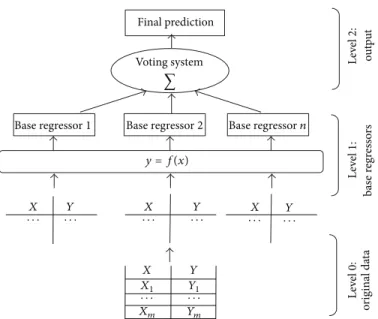
3.3. Ensemble Regressors. An ensemble regressor combines the predictions of a set of so-called base regressors using a

voting system [54], as we can see in Figure4. Probably the

three most popular ensemble techniques are Bagging [55],

(6)

×1

Figure 3: Model of the measured volume with a model tree.

Boosting, the ensemble regressor is formed from a set of weak base regressors, trained by applying the same learning algorithm to different sets obtained from the training set. In Bagging, each base regressor is trained with a dataset

obtained from random samplingwith replacement[55] (i.e.,

a particular instance may appear repeated several times or may not be considered in any base regressor). As a result, the base regressors are independent. However, Boosting uses all the instances and a set of weights to train each base regressor. Each instance has a weight pointing out how important it is to predict that instance correctly. Some base regressors can take weights into account (e.g., decision trees). Boosting trains base regressors sequentially, because errors for training instances in the previous base regressor are used for reweighting. The new base regressors are focused on instances that previous base regressors have wrongly predicted. The voting system for Boosting is also weighted by

the accuracy of each base regressor [57].

Random Subspaces follow a different approach: each base regressor is trained in a subset of fewer dimensions than the original space. This subset of features is randomly chosen for all regressors. This procedure is followed with the

intention of avoiding the well-known problem of thecurse of

dimensionalitythat occurs with many regressors when there are many features as well as improving accuracy by choosing

base regressors with low correlations between them. In total, we have used five ensemble regression techniques of the state of the art for regression, two variants of Bagging, one variant of Boosting, and Random Subspaces. The list of ensemble methods used in the experimentation is enumerated below.

(i) Bagging is in its initial formulation for regression. (ii) Iterated Bagging combines several Bagging

ensem-bles, the first one keeping to a typical construction and the others using residuals (differences between the real and the predicted values) for training purposes

[58].

(iii) Random Subspaces are in their formulation for regression.

(iv) AdaBoost.R2 [59] is a boosting implementation for

regression. Calculated from the absolute errors of

each training example,𝑙(𝑖) = |𝑓_𝑅(𝑥_𝑖) − 𝑦_𝑖|, the

so-called loss function, 𝐿(𝑖), was used to estimate the

error of each base regressor and to assign a suitable weight to each one. Let Den be the maximum value

of 𝑙(𝑖) in the training set; then three different loss

functions are used: linear,𝐿_𝑙(𝑖) = 𝑙(𝑖)/Den, square,

𝐿_𝑆(𝑖) = [𝑙(𝑖)/Den]2, and exponential,𝐿_𝐸(𝑖) = 1 − exp(−𝑙(𝑖)/Den).

(v) Additive regression is this regressor that has a learn-ing algorithm called Stochastic Gradient Boostlearn-ing

[60], which is a modification of Adaptive Bagging, a

hybrid Bagging Boosting procedure intended for least

squares fitting on additive expansions [60].

3.4. k-Nearest Neighbor Regressor. This regressor is the most representative algorithm among the instance-based learning. These kinds of methods forecast the output value using stored

values of the most similar instances of the training data [61].

The estimation is the mean of the k most similar training

instances. Two configuration decisions have to be taken:

(i) how many nearest neighbors to use to forecast the value of a new instance?

(ii) which distance function to use to measure the simi-larity between the instances?

In our experimentation we have used the most common definition of the distance function, the Euclidean distance, while the number of neighbors is optimized using cross-validation.

3.5. Support Vector Regressor. This kind of regressor is based on a parametric function, the parameters of which are optimized during the training process, in order to minimize

the RMSE [62]. Mathematically, the goal is to find a function,

𝑓(𝑥), that has the most deviation,𝜖, from the targets that

are actually obtained,𝑦_𝑖, for all the training data, and at the

same time is as flat as possible. The following equation is an example of SVR with the particular case of a linear function,

called linear SVR, where⟨⋅, ⋅⟩denotes the inner product in

the input space,𝑋:

(7)

Final prediction

Voting system

∑

Base regressor1 Base regressor2 Base regressorn

y = f(x)

Figure 4: Ensemble regressor architecture.

The norms of𝑤have to be minimized to find a flat

func-tion, but in real data solving this optimization problem can be

unfeasible. In consequence, Boser et al. [37] introduced three

terms into the formulation: the slack variables𝜉,𝜉∗andC, a

trade-off parameter between the flatness and the deviations

of the errors larger than 𝜖. In the following equation, the

optimization problem is shown that is associated with a linear SVR:

We have an optimization problem of the convex type that is solved in practice using the Lagrange method. The

equations are rewritten using theprimal objective function

and the corresponding constraints, a process in which the

so-calleddualproblem (see (8)) is obtained as follows:

maximize −1

From the expression in (8), it is possible to generalize

the formulation of the SVR in terms of a nonlinear function.

Instead of calculating the inner products in the original

feature space, a kernel function,𝑘(𝑥, 𝑥󸀠), that computes the

inner product in a transformed space was defined. This kernel

function has to satisfy the so-called Mercer’s conditions [63].

In our experimentation, we have used the two most popular

kernels in the literature [40]: linear and radial basis.

3.6. Artificial Neural Networks. We used the multilayer

per-ceptron (MLP), the most popular ANN variant [64], in our

experimental work. It has been demonstrated to be a

univer-sal approximator of functions [65]. ANNs are a particular case

of neural networks, the mathematical formulation of which is inspired by biological functions, as they aim to emulate

the behavior of a set of neurons [64]. This network has three

layers [66], one with the network inputs (features of the data

set), a hidden layer, and an output layer where the prediction is assigned to each input instance. Firstly the output of the

hidden layer,𝑦hide, is calculated from the inputs, and then the

output,𝑦hide, is obtained according to the expressions shown

in the following equation [66]:

𝑦hide = 𝑓net(𝑊1𝑥 + 𝐵1) 𝑦output= 𝑓output(𝑊2𝑦hide+ 𝐵2) ,

(9)

where𝑊₁is the weight matrix of the hidden layer,𝐵₁ is the

bias of the hidden layer,𝑊₂is the weight matrix of the output

layer (e.g., the identity matrix in the configurations tested),𝐵₂

is the bias of the output layer,𝑓netis the activation function

of the hidden layer, and𝑓outputis the activation function of

the output layer. These two functions depend on the chosen structure but are typically the identity for the hidden layer and

(8)

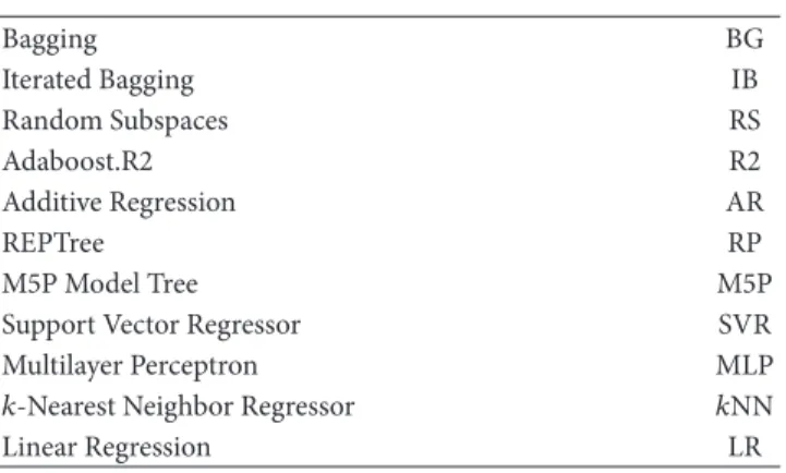
Table 6: Methods notation.

M5P Model Tree M5P

Support Vector Regressor SVR

Multilayer Perceptron MLP

𝑘-Nearest Neighbor Regressor 𝑘NN

Linear Regression LR

4. Results and Discussion

We compared the RMSE obtained for the regressors in

a 10×10 cross-validation, in order to choose the method that

is most suited to model this industrial problem. The

experi-ments were completed using the WEKA [20] implementation

of the methods described above.

All the ensembles under consideration have 100 base regressors. The methods that depend on a set of parameters are optimized as follows:

(i) SVR with linear kernel: the trade-off parameter,𝐶, in

the range 2–8;

(ii) SVR with radial basis kernel:𝐶from 1 to 16 and the

parameter of the radial basis function,gamma, from

10−5_to₁₀−2_;

(iii) multilayer perceptron: the training parameters

momentum, learning rate, and number of neuronsare optimized in the ranges 0.1–0.4, 0.1–0.6, and 5–15; (iv) kNN: the number of neighbours is optimized from 1

to 10.

The notation used to describe the methods is detailed in

Table6.

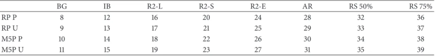
Regarding the notation, two abbreviations have been used

besides those that are indicated in Table6. On the one hand,

we used the suffixes “L,” “S,” and “E” for the linear, square, and exponential loss functions of Adaboost.R2, and, on the other

hand, the trees that are either pruned(𝑃)or unpruned(𝑈)

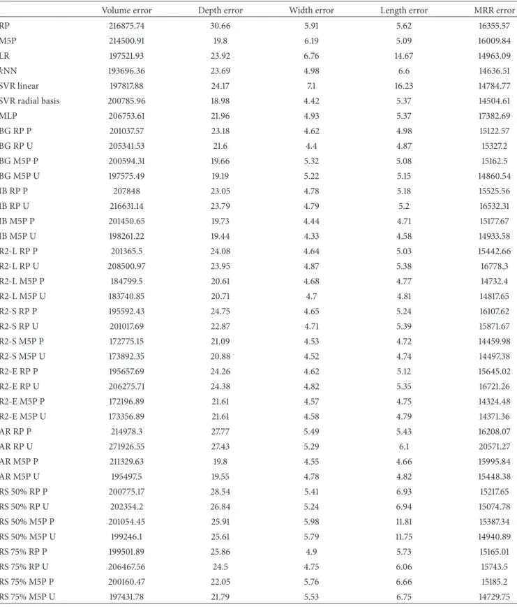
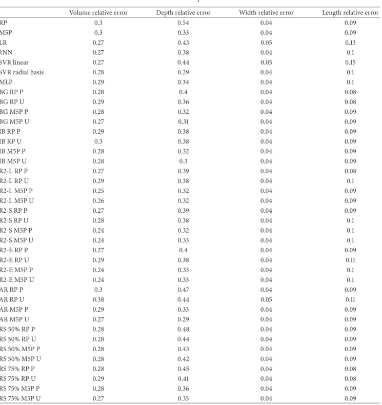
appear between brackets. Tables7,8, and9set out the RMSE

of each of the 14 outputs for each method.

Finally, a summary table with the best methods per output is shown. The indexes of the 39 methods that were tested are

explained in Tables 10 and11, and in Table12 the method

with minimal RMSE is indicated, according to the notation for these indexes. In the third column, we also indicate those methods that have larger RMSE, but, using a corrected

resampledt-test [67], the differences are not statistically

sig-nificative at a confidence level of 95%. Analyzing the second

column of Table 12, among the 39 configurations tested,

only 4 methods obtained the best RMSE for one of the 14 outputs: Adaboost.R2 with exponential loss and pruned M5P as base regressors—index 26—(5 times), SVR with radial

basis function kernel—index 6—(4 times), Iterated Bagging with unpruned M5P as base regressors—index 15—(4 times), and Bagging with unpruned RP as the base regressor - index 9—(1 time).

The performance of each method may be ranked. Table13

presents the number of significative weaker performances of each method, considering the 14 outputs modeled. The most robust method is Iterated Bagging with unpruned M5P as base regressors - index 15 -, as in none of the 14 outputs was it outperformed by other methods. Besides selecting the best method, it is possible to obtain some additional conclusions from this ranking table.

(i) Linear models like SVR linear—index 5— and LR— index 3—do not fit the datasets in the study very well. Both methods are ranked together at the middle of the table. The predicted variables therefore need methods that can operate with nonlinearities.

(ii) SVR with Radial Basis Function Kernel—index 6— is the only nonensemble method with competitive results, but it needs to tune 2 parameters. MLP—index 7—is not a good choice. It needs to tune 3 parameters and is not a well-ranked method.

(iii) For some ensemble configurations, there are dif-ferences in the number of statistically significative performances between the results from pruned and unpruned trees, while in other cases these differ-ences do not exist; in general, though, the results of unpruned trees are more accurate, specially with the top-ranked methods. In fact, the only regressor which is not outperformed by other methods in any output has unpruned trees. Unpruned trees are more sensitive to changes in the training set. So, the predictions of unpruned trees, when their base regressors are trained in an ensemble, are more likely to output diverse predictions. If the predictions of all base regressors agreed there would be little benefit in using ensembles. Diversity balances faulty predictions by some base regressors with correct predictions by others.

(iv) The top-ranked ensembles use the most accurate base regressor (i.e., M5P). All M5P configurations have fewer weaker performances than the corresponding RP configuration. In particular, the lowest rank was assigned to the AR - RP configurations, while AR M5P U came second best.

(v) Ensembles that lose a lot of information, such as RS, are ranked at the bottom of the table. The table shows that the lower the percentage of features RS use, the worse they perform. In comparison to other ensemble methods, RS is a method that is very insensitive to noise, so it can point to data that are not noisy. (vi) In R2 M5P ensembles, the loss function does not

appear to be an important configuration parameter. (vii) IB M5P U is the only configuration that never had

(9)

Table 7: Root mean squared error 1/3.

Volume Depth Width Length MRR

RP 216482.27 26.89 5.81 5.79 17166.73

M5P 210773.29 23.01 4.51 5.53 16076.33

LR 197521.89 23.84 7.04 14.73 15015.93

𝑘NN 193756.62 23.57 5.42 6.84 15842.42

SVR linear 197894.5 24.19 7.07 16.23 14800.32

SVR radial basis 200774.24 18.85 4.38 5.35 14603.37

MLP 207646.99 22.98 4.7 5.39 16292.43

BG RP P 200212.92 21.49 4.97 5.08 15526.79

BG RP U 205290.8 19.98 4.66 4.9 15603.89

BG M5P P 200636.57 20.61 4.43 5.27 15293.92

BG M5P U 197546.75 19.5 4.31 5.38 15022.1

IB RP P 202767.85 22.05 4.87 5.14 15677.57

IB RP U 219388.93 21.7 5.01 5.11 15911.96

IB M5P P 197833.83 20.8 4.42 4.88 15318.01

IB M5P U 195154.16 19.65 4.3 4.78 14830.83

R2-L RP P 191765.23 22.27 4.94 5.07 15788.47

R2-L RP U 206369.82 21.71 5.25 5.29 17004.31

R2-L M5P P 186843.92 20.81 4.37 4.84 15031.37

R2-L M5P U 181587.4 20.51 4.34 4.84 15209.01

R2-S RP P 193908.39 23.03 5.1 5.18 16007.43

R2-S RP U 200453.21 21.21 5.11 5.31 16401.24

R2-S M5P P 173117.72 20.83 4.49 4.71 15070.05

R2-S M5P U 173914.36 20.87 4.52 4.72 15245.81

R2-E RP P 192529.31 22.59 5.02 5.07 15854.03

R2-E RP U 205920.86 21.44 5.22 5.21 17318.45

R2-E M5P P 171056.22 21.25 4.53 4.66 15078.01

R2-E M5P U 172948.95 21.32 4.55 4.67 15090.23

AR RP P 215750.39 25.51 5.42 5.56 17249.82

AR RP U 274467.43 24.71 5.83 6.15 18628.28

AR M5P P 208805.84 22.27 4.44 5.08 16076.5

AR M5P U 194572.79 19.58 4.51 4.94 15538.29

RS 50% RP P 200526.36 26.58 5.68 7.74 15854.27

RS 50% RP U 201946.24 25.33 5.35 7.54 15669.28

RS 50% M5P P 201013.27 26.6 5.38 15.42 15402.77

RS 50% M5P U 199166.84 25.65 5.39 15.45 15349.84

RS 75% RP P 199270.03 23.33 5.27 5.98 15861.58

RS 75% RP U 207845.67 21.61 5.04 6.25 16251.64

RS 75% M5P P 199648.96 23.55 4.65 8.29 15227.87

RS 75% M5P U 197420.35 22.11 4.6 8.39 15295.71

Once the best data-mining technique for this industrial task is identified, the industrial implementation of these results can follow the procedure outlined below.

(1) The best model is run to predict one output, by changing two input variables of the process in small steps and maintaining a fixed value for the other inputs.

(2) 3D plots of the output related to the two varied inputs should be generated. The process engineer can extract information from these 3D plots on the best milling conditions.

(10)

Volume error Depth error Width error Length error MRR error

RP 216875.74 30.66 5.91 5.62 16355.57

M5P 214500.91 19.8 6.19 5.09 16009.84

LR 197521.93 23.92 6.76 14.67 14963.09

𝑘NN 193696.36 23.69 4.98 6.6 14636.51

SVR linear 197817.88 24.17 7.1 16.23 14784.77

SVR radial basis 200785.96 18.98 4.42 5.37 14504.61

MLP 206753.61 21.96 4.93 5.37 17382.69

BG RP P 201037.57 23.18 4.62 4.98 15122.57

BG RP U 205341.53 21.6 4.4 4.87 15327.2

BG M5P P 200594.31 19.66 5.32 5.08 15162.5

BG M5P U 197575.49 19.19 5.22 5.15 14860.54

IB RP P 207848 23.05 4.78 5.18 15525.56

IB RP U 216631.14 23.79 4.79 5.2 16532.31

IB M5P P 201450.65 19.73 4.44 4.71 15177.67

IB M5P U 198261.22 19.44 4.33 4.58 14933.58

R2-L RP P 201365.5 24.08 4.64 5.03 15442.66

R2-L RP U 208500.97 23.95 4.87 5.38 16778.3

R2-L M5P P 184799.5 20.61 4.68 4.77 14732.4

R2-L M5P U 183740.85 20.71 4.7 4.81 14817.65

R2-S RP P 195592.43 24.75 4.65 5.24 16107.62

R2-S RP U 201017.69 22.87 4.71 5.39 15871.67

R2-S M5P P 172775.15 21.09 4.53 4.72 14459.98

R2-S M5P U 173892.35 20.88 4.52 4.74 14497.38

R2-E RP P 195657.69 24.26 4.62 5.12 15645.02

R2-E RP U 206275.71 24.38 4.82 5.35 16721.26

R2-E M5P P 172196.89 21.61 4.57 4.75 14324.48

R2-E M5P U 173356.89 21.61 4.58 4.79 14371.36

AR RP P 214978.3 27.77 5.49 5.43 16208.07

AR RP U 271926.55 27.43 5.29 6.1 20571.27

AR M5P P 211329.63 19.8 4.55 4.66 15995.84

AR M5P U 195497.5 19.55 4.78 4.82 15448.38

RS 50% RP P 200775.17 28.54 5.41 6.93 15217.65

RS 50% RP U 202354.2 26.84 5.24 6.94 15074.78

RS 50% M5P P 201054.45 25.91 5.98 11.81 15387.34

RS 50% M5P U 199246.1 25.61 5.79 11.75 14940.89

RS 75% RP P 199501.89 25.86 4.9 5.73 15165.01

RS 75% RP U 206467.56 24.5 4.75 6.06 15743.5

RS 75% M5P P 200160.47 22.05 5.76 6.66 15185.2

RS 75% M5P U 197431.78 21.79 5.53 6.75 14729.75

and pulse intensity). In view of these restrictions, the engineer will wish to know the expected errors for the DES geometry depending on the laser parameters that can be changed. The rest of the inputs for the models (DES geometry) are

fixed at 70𝜇m depth, 65𝜇m width, and 0𝜇m length, and

PF is fixed at 45 KHz. Figure5shows the 3D plots obtained

(11)

Volume relative error Depth relative error Width relative error Length relative error

RP 0.3 0.54 0.04 0.09

M5P 0.3 0.33 0.04 0.09

LR 0.27 0.43 0.05 0.13

𝑘NN 0.27 0.38 0.04 0.1

SVR linear 0.27 0.44 0.05 0.15

SVR radial basis 0.28 0.29 0.04 0.1

MLP 0.29 0.34 0.04 0.1

BG RP P 0.28 0.4 0.04 0.08

BG RP U 0.29 0.36 0.04 0.08

BG M5P P 0.28 0.32 0.04 0.09

BG M5P U 0.27 0.31 0.04 0.09

IB RP P 0.29 0.38 0.04 0.09

IB RP U 0.3 0.38 0.04 0.09

IB M5P P 0.28 0.32 0.04 0.09

IB M5P U 0.28 0.3 0.04 0.09

R2-L RP P 0.27 0.39 0.04 0.08

R2-L RP U 0.29 0.38 0.04 0.1

R2-L M5P P 0.25 0.32 0.04 0.09

R2-L M5P U 0.26 0.32 0.04 0.09

R2-S RP P 0.27 0.39 0.04 0.09

R2-S RP U 0.28 0.38 0.04 0.1

R2-S M5P P 0.24 0.32 0.04 0.1

R2-S M5P U 0.24 0.33 0.04 0.1

R2-E RP P 0.27 0.4 0.04 0.09

R2-E RP U 0.29 0.38 0.04 0.11

R2-E M5P P 0.24 0.33 0.04 0.1

R2-E M5P U 0.24 0.33 0.04 0.1

AR RP P 0.3 0.47 0.04 0.09

AR RP U 0.38 0.44 0.05 0.11

AR M5P P 0.29 0.33 0.04 0.09

AR M5P U 0.27 0.29 0.04 0.09

RS 50% RP P 0.28 0.48 0.04 0.09

RS 50% RP U 0.28 0.44 0.04 0.09

RS 50% M5P P 0.28 0.43 0.04 0.09

RS 50% M5P U 0.28 0.42 0.04 0.09

RS 75% RP P 0.28 0.45 0.04 0.08

RS 75% RP U 0.29 0.41 0.04 0.08

RS 75% M5P P 0.28 0.36 0.04 0.09

RS 75% M5P U 0.27 0.35 0.04 0.09

Table 10: Index notation for the nonensemble methods.

1 2 3 4 5 6 7

RP M5P LR 𝑘NN SVR linear SVR radial basis MLP

5. Conclusions

In this study, extensive modeling has been presented with different data-mining techniques for the prediction of geo-metrical dimensions and productivity in the laser milling

(12)

Table 11: Index notation for the ensemble methods.

Table 12: Summary table.

Best

possible optimization strategies that industry might require for DES manufacturing: from high-productivity objectives to high geometrical accuracy in just one geometrical axis. By doing so, 14 data sets were generated, each of 162 instances.

Table 13: Methods ranking.

Indexes Methods

The experimental test clearly outlined that the geometry of the feature to be machined will affect the performance of the milling process. The test also shows that it is not easy to find the proper combination of process parameters to achieve the final part, which makes it clear that the laser micromilling of such geometries is a complex process to control. Therefore the use of data-mining techniques is proposed for the prediction and optimization of this process. Each variable to predict was modelled by regression methods to forecast a continuous variable.

The paper shows an exhaustive test covering 39 regression

method configurations for the 14 output variables. A10 × 10

cross-validation was used in the test to identify the methods

with a relatively better RMSE. A corrected resampledt-test

(13)

2.2

Forecast depth error:f(intensity, speed)

Speed

Forecast width error:f(intensity, speed)

Speed

Figure 5: 3D plots of the predicted depth and width’s errors from the Iterated Bagging ensembles.

RMSE was never significantly worse than the RMSE of any of the other methods for any of the 14 variables.

Future work will consider applying the experimental procedure to different polymers, magnesium, and other biodegradable and biocompatible elements, as well as to different geometries of industrial interest other than DES, such as microchannels. Moreover, as micromachining is a complex process where many variables play an important role in the geometrical dimensions of the machined workpiece, the application of visualization techniques, such as scatter plot matrices and start plots, to evaluate the relationships between inputs and outputs will help us towards a clearer understanding of this promising machining process at an industrial level.

Conflict of Interests

The authors declare that there is no conflict of interests regarding the publication of this paper.

Acknowledgments

The authors would like to express their gratitude to the GREP research group at the University of Girona and the Tecnol´ogico de Monterrey for access to their facilities during the experiments. This work was partially funded through Grants from the IREBID Project (FP7-PEOPLE-2009-IRSES-247476) of the European Commission and Projects TIN2011-24046 and TECNIPLAD (DPI2009-09852) of the Spanish Ministry of Economy and Competitiveness.

References

[1] K. Sugioka, M. Meunier, and A. Piqu´e,Laser Precision

Micro-fabrication, vol. 135, Springer, 2010.

[2] S. Garg and P. W. Serruys, “Coronary stents: current status,”

Journal of the American College of Cardiology, vol. 56, no. 10, pp. S1–S42, 2010.

[3] D. M. Martin and F. J. Boyle, “Drug-eluting stents for coronary

artery disease: a review,”Medical Engineering and Physics, vol.

33, no. 2, pp. 148–163, 2011.

[4] S. Campanelli, G. Casalino, and N. Contuzzi, “Multi-objective

optimization of laser milling of 5754 aluminum alloy,”Optics &

Laser Technology, vol. 52, pp. 48–56, 2013.

[5] J. Ciurana, G. Arias, and T. Ozel, “Neural network modeling and particle swarm optimization (PSO) of process parameters in pulsed laser micromachining of hardened AISI H13 steel,”

Materials and Manufacturing Processes, vol. 24, no. 3, pp. 358– 368, 2009.

[6] J. Cheng, W. Perrie, S. P. Edwardson, E. Fearon, G. Dearden, and K. G. Watkins, “Effects of laser operating parameters on metals

micromachining with ultrafast lasers,”Applied Surface Science,

vol. 256, no. 5, pp. 1514–1520, 2009.

[7] I. E. Saklakoglu and S. Kasman, “Investigation of micro-milling process parameters for surface roughness and micro-milling

depth,”The International Journal of Advanced Manufacturing

Technology, vol. 54, no. 5–8, pp. 567–578, 2011.

[8] D. Ashkenasi, T. Kaszemeikat, N. Mueller, R. Dietrich, H. J. Eichler, and G. Illing, “Laser trepanning for industrial

applica-tions,”Physics Procedia, vol. 12, pp. 323–331, 2011.

[9] B. S. Yilbas, S. S. Akhtar, and C. Karatas, “Laser trepanning of a small diameter hole in titanium alloy: temperature and stress

fields,”Journal of Materials Processing Technology, vol. 211, no. 7,

pp. 1296–1304, 2011.

[10] R. Biswas, A. S. Kuar, S. Sarkar, and S. Mitra, “A parametric study of pulsed Nd:YAG laser micro-drilling of gamma-titanium

aluminide,”Optics & Laser Technology, vol. 42, no. 1, pp. 23–31,

2010.

[11] L. Tricarico, D. Sorgente, and L. D. Scintilla, “Experimental investigation on fiber laser cutting of Ti6Al4V thin sheet,”

Advanced Materials Research, vol. 264-265, pp. 1281–1286, 2011. [12] N. Muhammad, D. Whitehead, A. Boor, W. Oppenlander, Z. Liu, and L. Li, “Picosecond laser micromachining of nitinol and

platinum-iridium alloy for coronary stent applications,”Applied

Physics A: Materials Science and Processing, vol. 106, no. 3, pp. 607–617, 2012.

[13] H. Meng, J. Liao, Y. Zhou, and Q. Zhang, “Laser micro-processing of cardiovascular stent with fiber laser cutting

system,”Optics & Laser Technology, vol. 41, no. 3, pp. 300–302,

(14)

[14] T.-C. Chen and R. B. Darling, “Laser micromachining of the materials using in microfluidics by high precision pulsed

near and mid-ultraviolet Nd:YAG lasers,”Journal of Materials

Processing Technology, vol. 198, no. 1–3, pp. 248–253, 2008. [15] D. Bruneel, G. Matras, R. le Harzic, N. Huot, K. K¨onig, and

E. Audouard, “Micromachining of metals with ultra-short Ti-Sapphire lasers: prediction and optimization of the processing

time,”Optics and Lasers in Engineering, vol. 48, no. 3, pp. 268–

271, 2010.

[16] M. Pfeiffer, A. Engel, S. Weißmantel, S. Scholze, and G. Reisse, “Microstructuring of steel and hard metal using femtosecond

laser pulses,”Physics Procedia, vol. 12, pp. 60–66, 2011.

[17] D. Karnakis, M. Knowles, P. Petkov, T. Dobrev, and S. Dimov, “Surface integrity optimisation in ps-laser milling of advanced

engineering materials,” inProceedings of the 4th International

WLT-Conference on Lasers in Manufacturing, Munich, Ger-many, 2007.

[18] H. Qi and H. Lai, “Micromachining of metals and thermal

barrier coatings using a 532 nm nanosecond ber laser,”Physics

Procedia, vol. 39, pp. 603–612, 2012.

[19] D. Teixidor, I. Ferrer, J. Ciurana, and T. ¨Ozel, “Optimization of

process parameters for pulsed laser milling of micro-channels

on AISI H13 tool steel,” Robotics and Computer-Integrated

Manufacturing, vol. 29, no. 1, pp. 209–219, 2013.

[20] I. Witten and E. Frank,Data Mining: Practical Machine Learning

Tools and Techniques, Morgan Kaufmann, 2nd edition, 2005.

[21] J. Han, M. Kamber, and J. Pei,Data Mining: Concepts and

Techniques, Morgan Kaufmann, 2006.

[22] A. J. Torabi, M. J. Er, L. Xiang et al., “A survey on artificial intelligence technologies in modeling of high speed end-milling

processes,” in Proceedings of the IEEE/ASME International

Conference on Advanced Intelligent Mechatronics (AIM ’09), pp. 320–325, Singapore, July 2009.

[23] M. Chandrasekaran, M. Muralidhar, C. M. Krishna, and U. S. Dixit, “Application of soft computing techniques in machining performance prediction and optimization: a literature review,”

The International Journal of Advanced Manufacturing

Technol-ogy, vol. 46, no. 5–8, pp. 445–464, 2010.

[24] A. K. Choudhary, J. A. Harding, and M. K. Tiwari, “Data mining in manufacturing: a review based on the kind of knowledge,”

Journal of Intelligent Manufacturing, vol. 20, no. 5, pp. 501–521, 2009.

[25] A. K. Dubey and V. Yadava, “Laser beam machining—a review,”

International Journal of Machine Tools and Manufacture, vol. 48, no. 6, pp. 609–628, 2008.

[26] B. F. Yousef, G. K. Knopf, E. V. Bordatchev, and S. K. Nikumb, “Neural network modeling and analysis of the material removal

process during laser machining,”The International Journal of

Advanced Manufacturing Technology, vol. 22, no. 1-2, pp. 41–53, 2003.

[27] S. Campanelli, G. Casalino, A. Ludovico, and C. Bonserio, “An artificial neural network approach for the control of the

laser milling process,”The International Journal of Advanced

Manufacturing Technology, vol. 66, no. 9–12, pp. 1777–1784, 2012.

[28] C. Jimin, Y. Jianhua, Z. Shuai, Z. Tiechuan, and G. Dixin,

“Parameter optimization of non-vertical laser cutting,” The

International Journal of Advanced Manufacturing Technology, vol. 33, no. 5-6, pp. 469–473, 2007.

[29] D. Teixidor, M. Grzenda, A. Bustillo, and J. Ciurana, “Mod-eling pulsed laser micromachining of micro geometries using

machine-learning techniques,”Journal of Intelligent

Manufac-turing, 2013.

[30] N. C. Oza and K. Tumer, “Classifier ensembles: select real-world

applications,”Information Fusion, vol. 9, no. 1, pp. 4–20, 2008.

[31] P. Santos, L. Villa, A. Re˜nones, A. Bustillo, and J. Maudes, “Wind

turbines fault diagnosis using ensemble classifiers,” inAdvances

in Data Mining. Applications and Theoretical Aspects, vol. 7377, pp. 67–76, Springer, Berlin, Germany, 2012.

[32] A. Bustillo and J. J. Rodr´ıguez, “Online breakage detection of multitooth tools using classifier ensembles for imbalanced

data,”International Journal of Systems Science, pp. 1–13, 2013.

[33] J.-F. D´ıez-Pastor, A. Bustillo, G. Quintana, and C. Garc´ıa-Osorio, “Boosting projections to improve surface roughness

prediction in high-torque milling operations,”Soft Computing,

vol. 16, no. 8, pp. 1427–1437, 2012.

[34] A. Bustillo, E. Ukar, J. J. Rodriguez, and A. Lamikiz, “Modelling of process parameters in laser polishing of steel components

using ensembles of regression trees,”International Journal of

Computer Integrated Manufacturing, vol. 24, no. 8, pp. 735–747, 2011.

[35] A. Bustillo, J.-F. D´ıez-Pastor, G. Quintana, and C. Garc´ıa-Osorio, “Avoiding neural network fine tuning by using ensemble

learning: application to ball-end milling operations,”The

Inter-national Journal of Advanced Manufacturing Technology, vol. 57, no. 5–8, pp. 521–532, 2011.

[36] S. Ferreiro, B. Sierra, I. Irigoien, and E. Gorritxategi, “Data mining for quality control: burr detection in the drilling

process,”Computers & Industrial Engineering, vol. 60, no. 4, pp.

801–810, 2011.

[37] B. E. Boser, I. M. Guyon, and V. N. Vapnik, “Training algorithm

for optimal margin classifiers,” inProceedings of the 5th Annual

Workshop on Computational Learning Theory, pp. 144–152, ACM, Pittsburgh, Pa, USA, July 1992.

[38] R. Beale and T. Jackson,Neural Computing: An Introduction,

IOP Publishing, Bristol, UK, 1990.

[39] A. Sykes,An Introduction to Regression Analysis, Law School,

University of Chicago, 1993.

[40] X. Wu, V. Kumar, Q. J. Ross et al., “Top 10 algorithms in data

mining,”Knowledge and Information Systems, vol. 14, no. 1, pp.

1–37, 2008.

[41] N. Tosun and L. ¨Ozler, “A study of tool life in hot

machin-ing usmachin-ing artificial neural networks and regression analysis

method,”Journal of Materials Processing Technology, vol. 124, no.

1-2, pp. 99–104, 2002.

[42] A. Azadeh, S. F. Ghaderi, and S. Sohrabkhani, “Annual elec-tricity consumption forecasting by neural network in high

energy consuming industrial sectors,”Energy Conversion and

Management, vol. 49, no. 8, pp. 2272–2278, 2008.

[43] P. Palanisamy, I. Rajendran, and S. Shanmugasundaram, “Pre-diction of tool wear using regression and ANN models in

end-milling operation,”The International Journal of Advanced

Manufacturing Technology, vol. 37, no. 1-2, pp. 29–41, 2008. [44] S. Vijayakumar and S. Schaal, “Approximate nearest neighbor

regression in very high dimensions,” inNearest-Neighbor

Meth-ods in Learning and Vision: Theory and Practice, pp. 103–142, MIT Press, Cambridge, Mass, USA, 2006.

(15)

[46] J. Yu, L. Xi, and X. Zhou, “Identifying source (s) of out-of-control signals in multivariate manufacturing processes using

selective neural network ensemble,”Engineering Applications of

Artificial Intelligence, vol. 22, no. 1, pp. 141–152, 2009.

[47] T. W. Liao, F. Tang, J. Qu, and P. J. Blau, “Grinding wheel con-dition monitoring with boosted minimum distance classifiers,”

Mechanical Systems and Signal Processing, vol. 22, no. 1, pp. 217– 232, 2008.

[48] S. Cho, S. Binsaeid, and S. Asfour, “Design of multisensor fusion-based tool condition monitoring system in end milling,”

The International Journal of Advanced Manufacturing

Technol-ogy, vol. 46, no. 5–8, pp. 681–694, 2010.

[49] S. Binsaeid, S. Asfour, S. Cho, and A. Onar, “Machine ensemble approach for simultaneous detection of transient and gradual

abnormalities in end milling using multisensor fusion,”Journal

of Materials Processing Technology, vol. 209, no. 10, pp. 4728– 4738, 2009.

[50] H. Akaike, “A new look at the statistical model identification,”

IEEE Transactions on Automatic Control, vol. 19, no. 6, pp. 716– 723, 1974.

[51] J. R. Quinlan, “Learning with continuous classes,” inProceedings

of the 5th Australian Joint Conference on Artificial Intelligence, vol. 92, pp. 343–348, Singapore, 1992.

[52] T. M. Khoshgoftaar, E. B. Allen, and J. Deng, “Using regression

trees to classify fault-prone software modules,”IEEE

Transac-tions on Reliability, vol. 51, no. 4, pp. 455–462, 2002.

[53] T. K. Ho, “The random subspace method for constructing

decision forests,”IEEE Transactions on Pattern Analysis and

Machine Intelligence, vol. 20, no. 8, pp. 832–844, 1998.

[54] T. G. Dietterichl, “Ensemble learning,” inThe Handbook of Brain

Theory and Neural Networks, pp. 405–408, 2002.

[55] L. Breiman, “Bagging predictors,”Machine Learning, vol. 24, no.

2, pp. 123–140, 1996.

[56] Y. Freund and R. E. Schapire, “Experiments with a new boosting

algorithm,” inProceedings of the 13th International Conference

on Machine Learning (ICML ’96), vol. 96, pp. 148–156, Bari, Italy, 1996.

[57] Y. Freund and R. E. Schapire, “A desicion-theoretic general-ization of on-line learning and an application to boosting,” inComputational Learning Theory, pp. 23–37, Springer, Berlin, Germany, 1995.

[58] L. Breiman, “Using iterated bagging to debias regressions,”

Machine Learning, vol. 45, no. 3, pp. 261–277, 2001.

[59] H. Drucker, “Improving regressors using boosting techniques,” inProceedings of the 14th International Conference on Machine Learning (ICML ’97), vol. 97, pp. 107–115, Nashville, Tenn, USA, 1997.

[60] J. H. Friedman, “Stochastic gradient boosting,”Computational

Statistics & Data Analysis, vol. 38, no. 4, pp. 367–378, 2002. [61] D. W. Aha, D. Kibler, and M. K. Albert, “Instance-based learning

algorithms,”Machine Learning, vol. 6, no. 1, pp. 37–66, 1991.

[62] A. J. Smola and B. Sch¨olkopf, “A tutorial on support vector

regression,”Statistics and Computing, vol. 14, no. 3, pp. 199–222,

2004.

[63] C. Cortes and V. Vapnik, “Support-vector networks,”Machine

Learning, vol. 20, no. 3, pp. 273–297, 1995.

[64] J. E. Dayhoff and J. M. DeLeo, “Artificial neural networks:

opening the black box,”Cancer, vol. 91, supplement 8, pp. 1615–

1635, 2001.

[65] K. Hornik, M. Stinchcombe, and H. White, “Multilayer