Discovery service in ad hoc networks using ants

Texto completo

(1)Instituto Tecnológico y de Estudios Superiores de Monterrey Campus Monterrey División de Tecnologı́as de Información y Electrónica Programa de Graduados. Discovery Service in Ad Hoc Networks Using Ants. THESIS Presented as a partial fulfillment of the requeriments for the degree of Master of Science in Electronic Engineering Major in Telecommunications. Carlos Crispı́n Garcı́a Terán December 2005.

(2) Discovery Service in Ad Hoc Networks Using Ants by. Carlos Crispı́n Garcı́a Terán. Thesis Presented to the Graduate Program of the Instituto Tecnologico y de Estudios Superiores de Monterrey as a partial fulfillment of the requeriments for the degree of Master of Science in Electronic Engineering major in Telecommunications. Instituto Tecnológico y de Estudios Superiores de Monterrey Campus Monterrey December 2005.

(3) Instituto Tecnológico y de Estudios Superiores de Monterrey Campus Monterrey Instituto Tecnologico y de Estudios Superiores de Monterrey Programa de Graduados. The members of the thesis committee recommended the acceptance of the thesis of Carlos Crispı́n Garcı́a Terán as a partial fulfillment of the requeriments for the degree of Master in Science in Electronic Engineering major in Telecommunications. THESIS COMMITTEE. César Vargas Rosales, Ph.D. Thesis advisor. José Ramón Rodrı́guez Cruz, Ph.D.. Jorge Carlos Mex Perera, Ph.D.. Synodal. Synodal. David Garza Salazar, Ph.D. Director of the Graduate Program. December 2005.

(4) To my dear parents, and brothers For their love, guidance, inspiration, patience, and support..

(5) Acknowledgments. I thank Instituto Tecnológico y de Estudios Superiores de Monterrey for the facilities provided. I am very grateful to my thesis advisor, César Vargas Rosales, Ph.D. for his interest, collaboration, patience, and support. I mention specially to José Ramón Rodrı́guez Cruz, Ph.D., and Jorge Carlos Mex Perera, Ph.D. for their valuable comments for the enhancement of this work. My friends, Hugo Tapia, Iván Gómez, Lorenzo Marciano, Mayela Barbosa, Milner Flores, and all my partners from CET.. Carlos Crispı́n Garcı́a Terán Instituto Tecnológico y de Estudios Superiores de Monterrey December 2005. vi.

(6) Chapter 1 Introduction. Recently, owing to advances of wireless communications people enjoy network services almost anywhere. Nevertheless, it is causing that the network resources be unsatisfactory for the number of users that increase continually. Besides, sometimes it is necessary to make use of network services in places where there is no fixed infrastructure available. For these reasons, the research of new technologies for more efficient service delivering is necessary. An ad-hoc wireless network is a network which consists of a collection of wireless nodes (all of which may be mobile) that dynamically create a topology among them without using any such infrastructure or administrative support, [1]. In addition, they are self-creating, self-organizing and self-administering, so they come into being solely by interactions among their constituent wireless mobile nodes and only such interactions are used to provide the necessary control and administration functions supporting such networks. Ad-hoc wireless networks offer unique benefits and versatility for certain environments and certain applications, but unfortunately numerous challenges must be overcome to realize the practical benefits of ad-hoc networking. These include effective routing, mobility management, power management, security, [1], [2], Quality of Service (QoS) requirements, [3], medium access and discovery services, [4], [5]. In this thesis, we pretend to fulfill both the routing and the discovery services in an ad-hoc network, making use of a routing model, which is based on the ant behavior.. 1.1. Objective. The objective of this work is to develop a discovery algorithm using ants for node, path and service discovery in an ad-hoc network that: 1. discovers neighbors automatically, establishes links and interacts with the network to 1.

(7) get information about addresses, routing, position, etc. 2. establishes the connection; find quickly ways to another nodes and gateways. 3. handles conditions concerning mobility, new links and link losses as well, new nodes and node losses, etc.. 1.2. Justification. Communication between people has growing enormous in the last years. Services like email, Internet, etc. have become a very important element in human life, for this reason, to know what services a network has is very important, because it depends on what information and devices you have available. It is significant to mention that by the present time, there is no true standard for service discovery designed specifically for ad-hoc wireless networks. For that, a service discovery method which provides automatic discovery of the desired services to the applications is particularly important in order to save the users from the trouble of the configuring task and take advantage of the full range of provided services.. 1.3. Thesis Organization. This thesis is organized as follows. In Chapter 2, an overview of the Ad Hoc networks is presented, also some service discovery are described too. Chapter 3 explains the Ant System and the proposed methods for service discovery. Chapter 4 give details of the results obtained from the simulation. Finally, Chapter 5 presents the conclusions and future works.. 2.

(8) Chapter 3 Model Description. In this chapter, we describe the model we will use to make our analysis. This model is based on the ants’ behavior, where the ants move across the network through randomly chosen pairs of nodes; leaving pheromones as they move through their journey, which help them to select their path at each intermediate node. Ant system presents good performance in scenarios with relative high activity and mobility; therefore it can help to overcome the blocking and the shortcut problems in ad hoc networks. We represent nodes inside a study region, which are generated using a Spatial Poisson Process. The Spatial Poisson Process depends on the intensity, where the intensity is defined as the mean number of events per unit area, that is E[γ] = λA where A is the area of the study region, λ is the value of the intensity, i.e., the average number of points per unit area, and γ is the number of events in the region. If the intensity does not vary over the region, the events follow a Poisson distribution with mean λA. (λA)k −(λA) e k = 0, 1, 2, ... (3.1) k! where X is the random variable for the number of nodes. Figure 3.1 shows a realization of P [X = k] =. this process for a square region with area equal to 10000 m2 , and intensity equal to 0.002 points/m2 , i.e., E[X]=20.. 3.1. Mobility Model. The initial positions of the nodes are chosen from a uniform random distribution over an area of 100 m by 100 m. In this area, each node moves with uniform speed between 0 17.

(9) Figure 3.1: Poisson process with mean equal to 20. and Vmax , besides a new direction is assigned uniformly distributed between 0 and 2π. The rectangular components of the speed for every node are calculated as follows Vx = V sin(θ). (3.2). Vy = V cos(θ). (3.3). Where Vx , and Vy are the rectangular components of the velocity vector of every node, and θ is the direction angle of each one (Figure 3.2). The displacement of the node in the x, and y axes is dx = Vx t. (3.4). dy = Vy t. (3.5). So the new position of the node will be given of the following form Px = Xoriginal + dx. (3.6). Py = Yoriginal + dy. (3.7). 18.

(10) Figure 3.2: Mobile nodes moving at random speeds and directions.. Where Xoriginal and Yoriginal are the actual coordinates of the node. Figure 3.3 shows the shift of position of a node.. 3.2. Beacon Packets. Beacon packets are also known as Hello signals. The main purpose of these packets is to inform each mobile node in the neighborhood about the other nodes, which are sent within a specified time period to ensure connectivity. Otherwise, the lack of messages from the node indicates the failure of that link. It is important to mention that when a mobile receives a hello message from a node, the node is added to the mobile’s routing table, and the mobile sends the node a copy of its routing table information (Figure 3.4).. 3.3. Neighbor Cache. Upon receipt of a beacon, a node records the beacon’s source ID in its neighbor table, which it scans at regular intervals to check the status of each of its neighbors. The neighbors are defined how the set of nodes in direct communication with the node in question, that is the nodes which are in the coverage of a node’s transmitter. These tables will be subsequently used by the routing algorithm.. 19.

(11) Figure 3.3: Shift of position of a node.. 3.4. Ant System. AS algorithms make use of simple agents called ants which iteratively construct candidate solution to a combinatorial optimization problem. Though any single ant moves essentially at random, it will make a decision on its direction based on the ”strength” of the pheromone on the paths that lie before it. As an ant traverses a path, it reinforces that path with its own pheromone, therefore the ”shortest” paths will maintain a higher amount of pheromone as opposed to the ”longer” paths. When applying Ant System (AS) to the TSP, arcs are used as solution components. A pheromone trail τi,j (t), where t is the iteration counter, is associated with each arc (i, j); these pheromone trails are modified during the run of the algorithm through pheromone trail evaporation and pheromone trail reinforcement by the ants. When applied to symmetric TSP instances, pheromone trails are also symmetric (τi,j (t) = τj,i (t)) while in applications to asymmetric TSPs (ATSPs) possibly (τi,j (t) 6= τj,i (t)). Initially, m ants are placed on m randomly chosen cities. Then, in each construction step, each ant moves, based on a probabilistic decision, to a city it has not yet visited. This probabilistic choice is biased by the pheromone trail τi,j (t), and by a locally available heuristic information ηi,j . The latter is a function of the arc length; AS and all other ACO algorithms for the TSP use ηi,j = 1/di,j . Ants prefer cities which are close and connected by arcs with a high pheromone trail and in AS an ant k currently located at city i chooses to go to city j with a probability, [20], 20.

(12) Figure 3.4: Diagram of Beacon Packets.. [τi,j (t)]α [ηi,j ]β , α β l∈θi [τi,l (t)] [ηi,l ]. Pi,j (t) = P. (3.8). where Pi,j (t) is the probability that edge (i, j) is chosen in iteration t, τi,j (t) is the concentration of pheromone associated with edge (i, j) in iteration t, ηi,j is the desirability of edge (i, j) and α and β are the parameters controlling relative importance of the pheromone intensity and desirability, respectively, for each ants’ decision. If α >> β then the algorithm will make decisions based mainly on the learned information, as represented by the pheromone and if β >> α the algorithm will act as a greedy heuristic selecting mainly the shortest or cheapest edges, disregarding the impact of these decisions on the final solution quality. 21.

(13) At the end of an iteration the pheromone on each edge is updated. The pheromone updating equation for AS is given by, [20],. τi,j (t + 1) = ρτi,j (t) + ∆τi,j (t),. (3.9). where ρ is the coefficient representing pheromone persistence (0 ≤ ρ ≤ 1) and ∆τi,j (t) is the pheromone addition for edge (i, j). The pheromone persistence factor is the mechanism by which the pheromone trails are decayed, enabling the colony to forget poor edges and increasing the probability of selecting good edges. For ρ−→1 only small amounts of pheromone are decayed between iterations and the convergence rate is slower, whereas for ρ−→0 more pheromone is decayed resulting in faster convergence. ∆τi,j (t) is a function of the solutions found at iteration t and is given by, [20],. ∆τi,j (t) =. m X. k ∆τi,j (t),. (3.10). k=1 k (t) is the pheromone addition laid on edge (i, j) by where m is the number of ants and ∆τi,j. the k th ant at the end of iteration t. This is given by, [20], ( k ∆τi,j (t). =. Q , f (Sk (t)). 0,. if (i, j) ∈ Sk (t), otherwise,. (3.11). where Q is the pheromone addition factor (a constant) and Sk (t) is the set of edges selected by ant k in iteration t and f (·) is the objective function. The main contributions of the Ant System are the following: * Positive feedback (Figure 3.5) is employed as a search and optimization tool. The idea is that, if at a given point an agent (ant) has to choose between different options, and the one actually chosen results to be good, then in the future that choice will appear more desirable than it was before. * Stigmergy can arise and be useful in distributed systems. In AS, the effectiveness of the search carried out by a given number of cooperative ants is greater than that of the search carried out by the same number of ants, each one acting independently from the others.. 22.

(14) Figure 3.5: Positive feedback mechanism forms a continuous circle, so shortest path is strongly marked with large probabilities (a great amount of pheromone).. 3.5. Pheromone Tables. The basic idea about the algorithm is the following. Artificial ants are continuously generated at any node in the network and are assigned random destination nodes. On their way to the respective destination node ants move around in the network and lay their pheromone trails. Every node has a pheromone table for every possible destination in the network, and each table has an entry for every neighbor so a node with k neighbors in a network with n nodes has a pheromone table with (n − 1) rows, where each row corresponds to a destination node, and has k entries where each entry corresponds to a neighbor node. The pheromone table contains probabilities (representing the strength of pheromone), which get regularly updated as soon as an ant reaches a node. Updating the probabilities thus represents pheromone laying. Figure 3.6 shows a possible network configuration and Table 3.1 the pheromone table.. Figure 3.6: Ants for network management.. 3.5.1. Pheromone Table Update. At every visited node k on the way back to the source node s, a backward agent updates some of the probabilities in the pheromone table of node k by using the travel information 23.

(15) Table 3.1: The pheromone table for node A. Destination Node B C D E. Neighbor Nodes B C D 0.73 0.12 0.15 0.10 0.82 0.08 0.07 0.15 0.78 0.36 0.51 0.13. in its memory which was collected and transformed by the forward agent. Figure 3.7 shows example route for a forward agent.. Figure 3.7: Route from source node to destination node. Node S represents the source node and node D represents the destination node. Nodes k + 1, k + 2, . . . are the visited nodes on the way from S to D. Tk+1 represents the travel time between S and k + 1, Tk+2 represents the travel time from k + 1 to k + 2 and so on. A forward agent will lay pheromone units and collect information during its moving from source node S to the destination. When the destination node D is reached, the forward agent activates the backward agent and transfers the whole route information to it. The backward agent will move from destination to source node (D→S). When the backward agent reaches node k + 1, it will update the probabilities in pheromone table of this node k + 1 through the pheromone units of the visited nodes. In the algorithm, the backward agent not only updates the probability to reach the destination node D from node k + 1 along node k + 2, but also updates the probabilities to reach every other node (k+3, k+4,. . ., k+n) on the sub-path to the destination node D along node k+2. The entry in the pheromone table corresponding to the node from which the ant has just come is increased according to the formula. 24.

(16) Pnew =. Pold + 4P . 1 + 4P. (3.12). The other entries in the table of this node are decreased according to. Pold , (3.13) 1 + 4P are the new probabilities, Pold is the old probability in the pheromone 0 Pnew =. 0 where Pnew , and Pnew. table, and 4P is the probability (or pheromone) increase. Note that (3.12) always increases the probability P , what means that every update is a positive feedback. This is like the pheromone of the ants, where every dropped pheromone increases the strength of a pheromone trail. By the other hand 4P is calculated using a relation of the pheromone units existing in the node. We call this routing method Ant Best Route (ABR) in where one of the primary requirements was encouraging the ants to find routes that are relatively short and of course avoid nodes that are heavily congested. The method consists in to send ants in a broadcast way so that they can find different routes to the destination node. It allows the probabilities for alternative choices to increase and select the best choice to the destination node owing to the cost as the number of links and nodes of a route, pheromone units, etc.. 3.6. Ant Multiple Routes (AMR). We propose another routing method, which is based in the probabilities of the links of the networks between the nodes, which we call Ant Multiple Routes (AMR). In this method ants can be launched from any node in the network, which has a random destination node and they move in a broadcast way until they reach the destination node. In every node visited they lay their pheromone trails and when the ant gets the destination node the forward ant generates a backward ant. The forward ant transfers all its memory to the backward ant and then destroys itself. As the result, the backward ant inherits the whole route information from the forward agent and its task is to go back to the source node s along the same path as the forward ant but in the opposite direction. At every visited node k on the way back to the source node s, a backward ant calculates both the probability of the link and the probability of the pheromone with respect to the previous node. To obtain the probability of the link (Figure 3.8), we take the coverage radius 25.

(17) R, and the Euclidian Distance dAB between the nodes, [27], i.e.,. Figure 3.8: Probability of link between nodes A y B.. P (link) = 1 − Fd (d),. (3.14). where Fd (d) = (. dAB 2 ). R. (3.15). (3.15) represents the probability of communication from a node to another one and depends on the distance.. Figure 3.9: Probability of the route. The probability of the pheromone is calculated using a relation of the pheromone units existing in the node. So that both probabilities are independent, hence the feasibility to use. 26.

(18) that link is. P (P heromone/Link) = P (P heromone) ∗ P (Link).. (3.16). Therefore the probability to use the route, is determined for the result of the feasibilities of use the links along the route (Figure 3.9). In important to mention that in this method we get several routes to the destination node so we have different options to reach the destination node and we can choose the best to get it.. 27.

(19) Chapter 2 Fundamentals of Ad Hoc Networks. A mobile ad-hoc network (MANET), [6], is defined as an autonomous system of mobile nodes connected by wireless links where these nodes are free to move randomly and organize themselves arbitrarily, thus the network’s topology may change quickly and unpredictably. The roots of ad-hoc networking can be traced back as far as 1968, when work on the ALOHA network was initiated (the objective of this network was to connect educational facilities in Hawaii), [7]. Although fixed stations were employed, the ALOHA protocol lent itself to distributed channel access management and hence provided a basis for the subsequent development of distributed channel access schemes that were suitable for ad-hoc networking. The ALOHA protocol itself was a single hop protocol that is, it did not inherently support routing and for this reason every node had to be within reach of all other participating nodes. Inspired by the ALOHA network and the early development of fixed network packet switching, DARPA began work in 1973 on the PRnet (packet radio network) a multihop network, [8]. Multihopping means that nodes cooperated to relay traffic on behalf of one another to reach distant stations that would otherwise have been out of range. PRnet provided mechanisms for managing operation centrally as well as on a distributed basis, so, as an additional benefit, it was realized that multihopping techniques increased network capacity, since the spatial domain could be reused for concurrent but physically separate multihop sessions. Although many experimental packet radio networks were later developed, these wireless systems did not ever really take off in the consumer segment. When developing IEEE 802.11 a standard for wireless local area networks (WLAN) the Institute of Electrical and Electronic Engineering (IEEE) replaced the term packet radio network with ad-hoc network. Because an ad-hoc network does not use a centralized administration, nodes can enter/leave the network as they wish. Moreover, owing to the limited transmitter range of the nodes multiple hops may be needed to reach other nodes, so that every node in the network 3.

(20) must act both as a host and as a router. It is important to mention that in contrast to traditional wireline or wireless networks, an ad-hoc network could be expected to operate in a network environment in which some or all the nodes are mobile, for this reason, the network functions must run in a distributed fashion, since nodes might suddenly disappear from, or show up in, the network. However, the same basic user requirements for connectivity and traffic delivery that apply to traditional networks will apply to ad-hoc networks. In general, the principal characteristics of a mobile ad-hoc network are: * Dynamic topology: network topology change rapidly owing to the free movement of the nodes. * Bandwidth constraint: the bandwidth of wireless links is in general small as compared to fixed connections. * Energy constraint: the set of functions offered by a node depends on its available power, so that energy conservation is important. * Security: is an issue of critical importance for most networks and mobile ad-hoc networks are no exception. * Multiple routes: since the topology may change rapidly, the maintenance of multiple routes may ensure continuous reach ability of the nodes.. 2.1. Routing. Routing is fundamental in communication network control, because it means the action of addressing data traffic between pairs of source-destination nodes. In conjunction with a flow control, congestion and admission, routing determines the total network performance, in terms of quality and amount of offered services.. 2.1.1. Routing Classification. Routing protocols can be classified, [9], into different categories depending on the properties: - Centralized vs. Distributed. - Static vs. Adaptive. - Reactive vs. Proactive. 4.

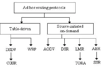
(21) One way to categorize the routing protocols is to divide them into centralized and distributed algorithms. In centralized algorithms all route choices are made at a central node, while in distributed algorithms the computation of routes is shared among the network nodes. Another classification of routing relates to whether they change routes in response to the traffic input patterns. In static algorithms the route used by source-destination pairs is fixed regardless of traffic conditions and it can only change in response to a node or link failure. This type of algorithms can not achieve high throughput under a broad variety of traffic input patterns. Adaptive algorithms, most major packet networks use some form of this routing, where the routes used to route between source-destination pairs may change in response to congestion. The last classification and most related to ad-hoc networks, which classify them as either proactive or reactive. Proactive protocols attempt to continuously evaluate the routes within de network, so that when a packet needs to be forwarded, the route is already known and can be immediately used. On the other hand, reactive protocols invoke a route determination procedure on demand only, thus when a route is needed some sort of global search procedure is employed. Proactive schemes have the advantage that when a route is needed, the delay before actual packets can be sent in very small but they needs time to coverage to a steady state. This can cause problems if the topology is changing frequently.. 2.1.2. Ad Hoc Routing Protocols. Compared to wired networks with static nodes, an ad-hoc network require a highly adaptive routing scheme to cope with the high rate of topology changes. This implies that the protocols must deal with the typical limitations of these networks, which include high power consumption, low bandwidth, and high error rates. As shown in Figure 2.1, these routing protocols may generally be: * Table-driven. * Source-initiated (demand-driven). Table-driven routing protocols, [10], attempt to maintain consistent, up to date routing information from each node to every other node in the network. These protocols require each node to maintain one or more tables to store routing information and they respond to changes in network topology by propagating updates throughout the network in order to maintain a consistent network view. Some of these protocols are Destination-Sequenced Distance Vector Routing (DSDV), [11], Wireless Routing Protocol (WRP), [12], and Clusterhead Gateway Switch Routing (CGSR), [13].. 5.

(22) Figure 2.1: Categorization of ad-hoc routing protocols. Source-initiated routing, [10], creates routes only when desired by the source node. When a node requires a route to destination, it initiates a route discovery process within the network and this process is executed until a route is found or all possible route permutations have been examined. Once a route has been established, it is maintained by a route maintenance procedure until either the destination becomes inaccessible along every path from the source or until the route is no longer desired. Some of these protocols are Ad-hoc On-Demand Distance Vector Routing (AODV), [14], Dynamic Source Routing (DSR), [15], Lightweight Mobile Routing (LMR), [16], and Associativity-Based Routing (ABR), [17]. It is important to say that in general, proactive protocols are suitable to high changing but not large environments, where routes have reduced lifetime due to a changing topology or node mobility. On the other hand, reactive schemes work better in environments where changes in topology do not occur frequently, having a higher route discovery delay in large networks. Due to these characteristics, neither reactive nor proactive protocols are proper to realize an effective routing in ad-hoc networks, doing necessary more suitable routing protocols that could be reliable in a mobile as in a static network and in addition could work in large as in a small size networks as well. An emerging routing tendency consists of mixing the characteristics of proactive and reactive, that is, protocols which working jointly at different levels of the network topology. Zone Routing Protocol (ZRP), [18], is one of this kind of hybrid protocol, which manages reduced proactive routing areas (zones), whereas the complete network consists of many of these zones and the communication between zones is in a reactive manner, using a pseudo 6.

(23) hierarchical network scheme.. 2.2. Quality of Service (QoS) Issues for Ad Hoc Networks. QoS can be defined as a guarantee by the network to satisfy a set of predetermined service performance constraints for the user in terms of the end-to-end delay statistics, available bandwidth, probability of packet loss, etc. where, of course, enough network resources must be available during the service invocation to keep the guarantee. For this, the first essential task is to find a suitable path through the network, or route, between the source and destination that will have the necessary resources available to meet the QoS constraints for the desired service. Once a route has been selected for a specific flow, the necessary resources, (bandwidth, buffer space in routers, etc.) must be reserved for the flow, which will not be available to other flows. Consequently, the amount of remaining network resources available to accommodate the QoS requests of other flows will have to be recalculated and propagated to all other pertinent nodes as part of the topology update information. QoS routing executes both tasks, [3], for this, it dependents on the accurate availability of the current network state. The first is the local state information maintained at each node, which includes queuing delay and the residual CPU capacity for the node, as well as the propagation delay, bandwidth and some form of cost metric for each of its outgoing links. The totality of local state information for all nodes constitutes the global state of the network, which is also maintained at each node. While the local state information may be assumed to be always available at any particular node, the global state information is constructed by exchanging the local state information for every node among all the network nodes at appropriate moments. The process of updating the global state information is also loosely called topology updates and it may significantly affect the QoS performance of the network due to updates consume network bandwidth, besides frequently changing routes could increase the delay jitter experienced by the users. For determining an optimal path satisfying the QoS constraints three distinct routefinding techniques are used, which are source routing, destination routing, and hierarchical routing. In source routing, a feasible path is locally computed at the source node using the locally stored global state information and then all other nodes along this feasible path are notified by the source of their adjacent preceding and successor nodes. In distributed or hop-by-hop routing, the source as well as other nodes are involved in path computation 7.

(24) by identifying the adjacent router to which the source must forward the packet associated with the flow. Hierarchical routing uses the aggregated partial global state information to determine a feasible path using source routing where the intermediate nodes are actually logical nodes representing a cluster.. 2.3. Ant System. Ants are small insects, often black or brown, that live in large groups and are thought of as hard working. They have a small amount of cognitive capability, limited individual capabilities and react instinctively in a probabilistic way to their perception of their immediate environment. They find the shortest path between the nest and a food source by laying down a trail of an attracting substance, called pheromone and depending on the species, ants in nature may lay pheromone trails when traveling from the nest to food or from food to the nest or when traveling in either direction, which they follow with a fidelity that is a function of the trail strength. The strength of the trail they lay is a function of the rate at which they make deposits and the amount per deposit. Since pheromones evaporate and diffuse away, the strength of the trail when another ant encounters it is a function of the original strength and the time since the trail was laid. Most trails consist of several superimposed trails from many different ants, which may have been laid at different times; it is the composite trail strength, which is sensed by the ants, [28].. Figure 2.2: Ants arrive at a decision point. Consider Figure 2.2, ants arrive at a decision point in which they have to decide whether to turn left or right. Since they have no clue about which is the best choice, they choose randomly and it can be expected that, on average, half of the ants decide to turn left and the 8.

(25) other half to turn right. This happens both to ants moving from left to right and vice versa, but if there is pheromone present, there is a higher probability of an ant choosing the path with the higher pheromone concentration. Figures 2.3 and 2.4 show what happens in the immediately following instants, supposing all ants walk at approximately the same speed. The ants that chose the upper branch have arrived at their destination, while the ones that chose the longer branch are still on their way.. Figure 2.3: Some ants choose the upper path and some the lower path in a random choice. The lines on the paths represent the pheromone trails. If at the moment of the situation in Figure 2.4 another ants arrive and have to choose between the two paths, they are more likely to choose the upper path, because that is where the concentration of pheromone is higher, this means that the amount of pheromone on the shorter path is more likely to be reinforced again. In this way, a stronger pheromone trail will arise on the upper path and so an increasing proportion of ants will select the path. As fewer ants choose the longer path and the existing pheromone slowly evaporates, the trail on the longer path will weaken and eventually disappear. The above behavior of real ants has inspired ant system, an algorithm in which a set of artificial ants cooperate to the solution of a problem by exchanging information via pheromone deposited on graph edges. The Ant System, [19], is a general-purpose heuristic algorithm, which can be used to solve diverse combinatorial optimization problems. This work has been lead by Marco Dorigo at the Politecnico di Milano, Italy.. 9.

(26) Figure 2.4: Situation several moments later. The lines on the paths represent the pheromone trails.. 2.3.1. Motivations for the Ant System. The Ant System (AS) has the following desirable characteristics: 1. It is versatile, in that it can be applied to similar versions of the same problem. For example, there is a straightforward extension from the traveling salesman problem (TSP) to the asymmetric traveling salesman problem (ATSP). 2. It is robust and general-purpose. With minimal modifications, it can be applied to other combinatorial optimization problems such as the job shop scheduling problem (JSP) and the quadratic assignment problem (QAP). 3. It is a population-based heuristic. As such, it allows the exploitation of positive feedback as a search mechanism, so, it makes the system amenable to similar implementations. The AS is an example of a distributed search technique. Search activities are distributed over ant-like agents, which are entities with very simple basic capabilities and in a metaphorical and highly stylized way, mimic the behavior of real ants. The research inspiration for the AS arises from the work of ethnologists, who attempted to understand how almost blind animals like ants could manage to establish shortest route paths from their colony to feeding sources and back.. 2.3.2. Applications of the Ant System. Most work on the Ant System has been applied to the Traveling Salesman Problem. Dorigo shows that the Ant System can be applied to the TSP, [19], [20], and other problems,. 10.

(27) which can be expressed in graph-partitioning terms. Dorigo’s conclusions on the results of the Ant System on the TSP are: 1. Within the range of parameter optimality, the algorithm always finds very good solutions for all of the tested problems. 2. The algorithm quickly finds good solutions, while not exhibiting stagnation behavior, the ants continue to search for new possibly better tours. 3. With increasing problem size, the sensitivity of the parameter values to the problem dimension has been found acceptable. The work on the TSP is directly transferable to the asymmetric TSP, which is significantly more difficult than the TSP. Typically the TSP can be solved for graphs with several thousand nodes, while the ATSP is only solved optimally in cases where there are several dozen nodes. The Ant System has also been applied to the Quadratic Assignment Problem (QAP) and the Job Shop Scheduling Problem (JSP), which required very few changes to the algorithm, as long as the problem could be stated in an appropriate graph notation.. 2.3.3. Routing. The motivation for exploiting the ant metaphor for routing in telecommunications networks arises from the fact that routing systems frequently depend upon global information for their efficient operation. Ant systems do not need such global information, relying instead upon pheromone traces that are laid down in the network as the ant, or agent, moves through the network. Global information is frequently out of date and transmission of the information required from one node to all others consumes considerable network bandwidth. In, [21], they proposed an Ant Based Algorithm for Control Management in Ad-hoc Networks, making use of the swarm intelligence into the network routing problems with the objective of improve the performance of these networks. They got better performance using Ant Routing Algorithm than other protocols like Zone Routing Protocol (ZRP) in scenarios with relative high activity and mobility, and it is important to say that, the contribution of this thesis is the employment of positive feedback as a search and optimization tool in routing schemes, and how the synergy can arise and be useful in distributed systems using cooperative ants, each one acting independently from the others, all of these in a telecommunication network environment.. 11.

(28) 2.4. Service Discovery. With the raising number of network services, automatic service discovery will be a very important feature in future networks scenarios, because devices may automatically discover network services including their properties and services may advertise their existence in a dynamic way. Service discovery protocol (SDP) enable users of a communication network to find service, applications and devices that are available in the network, that is, its purpose is to allow nodes on an infrastructure less wireless network find services offered by other nodes in the network, which fulfill a certain task. This feature is especially useful for mobile users in a foreign network and for groups of users that form a spontaneous (ad-hoc) wireless network. Service discovery protocols (SDP) for wireless ad-hoc networks are classified in two categories: proactive (or push-based) and reactive (or pull-based) SDPs. Proactive SDP uses a broadcast mechanism, where each node unsolicitly advertises the services it can offer to the rest of the nodes in the network. In case of reactive SDPs, each node queries other nodes for the services it requires. It’s important to mention that a problem with proactive SDPs is large bandwidth requirement for message broadcasts, in addition, there is a potential for long latency in discovering services, especially when nodes take turns in sending broadcast messages. By the other hand, reactive SDPs suffer from bandwidth overhead (but less than that for proactive SDPs) and long latency (longer than that for proactive SDPs) to find the required services. Finally, both the proactive and reactive SDPs consume the limited battery power of the network nodes. A variety of service discovery protocols are currently under development, [29]. The most well known are: - Service Location Protocol (SLP) developed by the IETF. - Jini, which is Sun’s Java-based approach to service discovery. - Salutation. - Microsoft’s Universal Plug and Play (UPnP). - Bluetooth Service Discovery Protocol (SDP).. 2.4.1. Service Location Protocol (SLP). The Service Location protocol (SLP), [10], [22], is an Internet Engineering Task Force standard for enabling IP networks-based applications to automatically discover the location of a required service. The SLP architecture consists of three main components: 12.

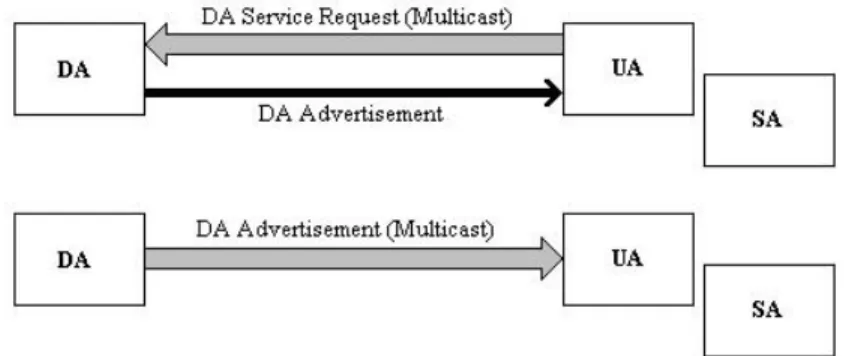
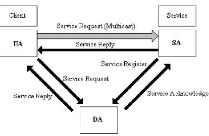
(29) * User Agent (UA): it is a software entity and it acts as an agent to search for requested services. It can even cache service information so that subsequent requests can be fulfilled immediately, and is responsible for interrogating service availability. In addition it does not inform the user what access methods to be used, but merely points the user toward the service provider to contact. As shown in Figure 2.5, the UA can contact an SA or DA for service information. * Directory Agent (DA): to allow a service location architecture to scale, having just a UA and an SA is insufficient. With a large network, a UA may receive thousands of replies about the service it is requesting. This can give rise to discovery implosion and is particularly bad for a wireless environment. The introduction of a DA helps to alleviate this problem. The DA consolidates all the service replies and catches them into a directory. As shown in Figure 2.5, acting as a proxy, the DA can reply back to the UAs directly, hence avoiding the discovery acknowledgment implosion problem. Another way to address scalability is the use of administrative domains, since UAs searching for services within a permitted administrative domain only see those devices available in that domain. Administrative domains, therefore, limit the visibility of services. * Service Agent (SA): the SA acts as an agent for the service provider. It advertises available services either directly to the UAs or to Das. If affiliated with certain Das, an SA can periodically register available services with the DAs.. Figure 2.5: The interactions between a DA and an(a) UA/SA in SLP. Figure 2.6 shows the interactions between three agents. When a new service connects to a network, the SA contacts the DA to advertise its existence (Service Registration). When a user needs a certain service, the UA queries the available services in the network from the DA (Service Request). After receiving the address and characteristics of the desired service, the user may finally utilize the service.. 13.

(30) Figure 2.6: Interactions among Das, Uas, and SAs. Before a client (UA or SA) is able to contact the DA, it must discover the existence of the DA. There are three different methods for DA discovery: static, active, and passive. With static discovery, SLP agents obtain the address of the DA through DHCP (Dynamic Host Configuration Protocol, [23]). In active discovery, UAs and SAs send service requests to the SLP multicast group address, where a DA listening on this address will eventually receive a service request and respond directly (via unicast) to the requesting agent. In case of passive discovery, DAs periodically send out multicast advertisements for their services, so that UAs and SAs learn the DA address from the received advertisements and are now able to contact the DA themselves via unicast. It is important to note that the DA is not mandatory. In fact, it is used especially in large networks with many services, since it allows categorizing services into different groups (scopes), but in smaller networks it is more effective to deploy SLP without a DA. SLP has therefore two operational modes, depending on whether a DA is present or not. If a DA exists on the network (as shown in Figure 2.6), it will collect all service information advertised by SAs, so that UAs will send their Service Requests to the DA and receive the desired service information. If there is no DA, UAs repeatedly send out their Service Request to the SLP multicast address. All SAs listen for these multicast requests and if they advertise the requested service, they will send unicast responses to the UA. Furthermore, SAs multicast an announcement of their existence periodically, so that UAs can learn about the existence of new services. Services are advertised using a Service URL and a Service Template. The Service URL contains the IP address of the service, the port number and path. Service Templates specify the attributes that characterize the service and their default values. 14.

(31) 2.4.2. Jini Protocol. Jini, [10], [24], technology is an extension of the programming language Java and has been developed by Sun Microsystems. It addresses the issue of how devices connect with each other in order to form a simple ad-hoc network and how these devices provide services to other devices in this network. Each Jini device is assumed to have a Java Virtual Machine (JVM) running on it. The Jini architecture principle is similar to that of SLP, because devices and applications register with a Jini network using a process called Discovery and Join, so to join a Jini network, a device or application places itself into the Lookup Table on a lookup server, which is a database for all services on the network (similar to the DA in SLP). Besides pointers to services, the Lookup Table in Jini can also store Java-based program code for these services, this means that services may upload device drivers, an interface and other programs that help the user to access the service. When a client wants to utilize the service, the object code is downloaded from the Lookup Table to the JVM of the client, whereas a service request in SLP returns a Service URL, the Jini object code offers direct access to the service using an interface known to the client. This code mobility replaces the necessity of pre-installing drivers on the client.. 2.4.3. Salutation Protocol. The Salutation, [10], [25], architecture is being developed by Salutation Consortium, which is an open industry consortium. Salutation is an architecture for looking up, discovering and accessing services and information and its goal is to solve the problems of service discovery and utilization among a broad set of applications and equipment in an environment of widespread connectivity and mobility. The Salutation architecture defines an entity called the Salutation Manager (SLM) that functions as a directory of applications, services and devices, generically called Networked Entities. The SLM allows networked entities to discover and to use the capabilities of the other networked entities.. 2.4.4. Universal Plug and Play Protocol (UPnP). Universal Plug and Play (UPnP), [26], is being developed by an industry consortium, which has been founded and is lead by Microsoft. Its usage is proposed for small office or home computer networks, where it enables peer-to-peer mechanisms for auto configuration of devices, service discovery, and control of services and in UPnP’s current version 15.

(32) (release 0.91) there is no central service register, such as the DA in SLP or the lookup table in Jini. The Simple Service Discovery Protocol (SSDP), [22], is used within UPnP to discover services and SSDP uses HTTP over UDP and is thus designed for usage in IP networks.. 2.4.5. Bluetooth Service Discovery Protocol (SDP). Bluetooth Service Discovery, [10], is a new short-range wireless transmission technology. The Bluetooth protocol stack contains the Service Discovery Protocol (SDP), which is used to locate services provided by or available via a Bluetooth device and it is based on the Piano platform by Motorola, it has been modified to suit the dynamic nature of ad-hoc communications. It addresses service discovery specifically for this environment and thus focuses on discovering services, where it supports the following inquiries: search for services by service type, search for services by service attributes and service browsing without a priori knowledge of the service characteristics, but SDP does not include functionality for accessing services. Once services are discovered with SDP they can be selected, accessed and used by mechanisms out of the scope of SDP, for example by other service discovery protocols such as SLP and Salutation.. 16.

(33) Chapter 4 Numerical Results. In this chapter, we present the results obtained with the routing models described in the last chapter using the ant system in a wireless Ad Hoc Network. Also, we present the parameters, and considerations made in the simulation of the algorithms.. 4.1. Simulation. In the simulation, we consider different number of nodes, which are created following a Spatial Poisson distribution. All the nodes transmit with the same power level in all scenarios and the links between the nodes are established considering that the reception power (PR ) be greater than the threshold power (Pthreshold ). To know the topology of the network, beacons are sent every t seconds (tbeacon ) and in this way the nodes can know both their neighbors at one hop and other nodes that belong to the network. The nodes move independently with different velocities and direction inside the study area, which is the same in all the scenarios; also we use the ping-pong mobility model to keep the nodes from leaving the study area (Figure 4.1). The maximum transmission radius of the nodes depends on the power intensity, where the intensity is defined as the mean number of events per unit area, that is. λ = E[γ]/A,. (4.1). where λ is the value of the intensity, γ is the number of events in the region, and A is the area of the study region. The probability of not having a neighbor inside the transmission radius is. 28.

(34) Figure 4.1: Closed coverage area.. 2. P (N = 0) = e−λπr ,. (4.2). where r is the transmission radius. We choose r according to 2. e−λπr < 0.01 That is that the probability is less than 1%. Also each node generates ants every t seconds (tant ), and every ant involves a source node, a destination node, and ant life time measured in time steps. The ants are sent to random destinations in a broadcast way and their objective is to find routes to the destination node. In every node visited the ants lay their pheromone, which evaporates a certain percentage every time step. The characteristics of the nodes and parameters used in the different scenarios of the simulation as well as notation are presented in Table 4.1. In the next sections, we propose some scenarios where we used the fixed parameters described in Table 4.1, also other not fixed (Table 4.2) like the time between beacons (tbeacon ), the time between ants (tants ), the life time of the ant, the maximum transmission radius (r), the minimum received power at a distance r (Pthreshold ), the maximum speed that reaches the nodes (Vmax ), etc., to analyze the routing methods.. 29.

(35) Table 4.1: Fixed parameters for the mobile ad hoc network. Coverage area (Xmax , Ymax ) Transmission power (PT x ) Path loss exponent (α) Maximum node angle (θmax ) Data packet length (L) Transmission rate (C) Buffer size in packets Pheromone ant evaporation every time step (perevap). 100x100 m 5 × 10−3 w 4 3600 512000 bits 10 Mbps 64 packets 5%. Table 4.2: Not fixed parameters for the mobile ad hoc network. Node population (Ntot ) Maximum node speed (Vmax ) Beacon time (tbeacon ) Maximum transmission radius (r) Minimum received power (Pthreshold ) Ant time (tants ) Life time ant Minimum pheromone. 30.

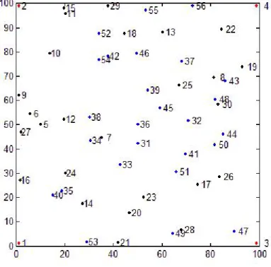
(36) 4.2. Proposed Scenarios. In this section we propose some scenarios where the objective is to compare the behavior of the routing method when we change some parameters like the time between ants, the life time of the ants, etc.. 4.2.1. Scenario 1. In the first scenario, we use the topology of Figure 4.2. In the topology, we have a density equal to 0.005 (γ=0.005 nodes/m2 ), and the nodes are randomly distributed into the area according to a Complete Spatial Randomness (CSR). The simulation time is about 150 sec and there is no mobility in this scenario, the nodes located on the corners are considered service nodes. We analyze the routing behavior between the service node number 4 (position (99, 99)), and node number 36 (position (50, 50)) where node 36 is considered the source node and node 4 the destination node. The parameters employed are shown in Table 4.3. It is important to mention that all the nodes are sending ants to their destinations which are located to 2 or more hops every ant time (tants ).. Figure 4.2: Scenario with with mean equal to 50.. 31.

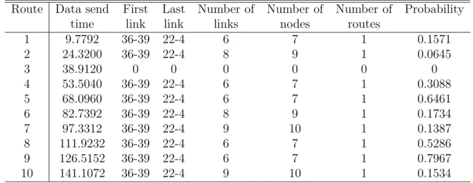
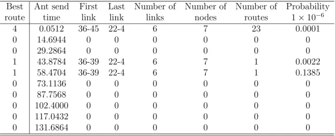
(37) Table 4.3: Not fixed parameters for scenario 1. Simulation time Node population (Ntot ) Maximum node speed (Vmax ) Beacon time (tbeacon ) Maximum transmission radius (r) Minimum received power (Pthreshold ) Ant time (tants ) Minimum pheromone. 150 sec 56 0 m/s 20 sec 18 m 4.7630 × 10−8 w 15 sec 7 units. Table 4.4: Results of scenario 1 using Ant Best Route (ABR). Route 1 2 3 4 5 6 7 8 9 10. Data send time 9.7792 24.3200 38.9120 53.5040 68.0960 82.7392 97.3312 111.9232 126.5152 141.1072. First Last link link 36-39 22-4 36-39 22-4 0 0 36-39 22-4 36-39 22-4 36-39 22-4 36-39 22-4 36-39 22-4 36-39 22-4 36-39 22-4. Number of links 6 8 0 6 6 8 9 6 6 9. Number of nodes 7 9 0 7 7 9 10 7 7 10. Number of routes 1 1 0 1 1 1 1 1 1 1. Probability 0.1571 0.0645 0 0.3088 0.6461 0.1734 0.1387 0.5286 0.7967 0.1534. Table 4.4 shows the results obtained with Ant Best Route (ABR), and Table 4.5 the results obtained with Ant Multiple Routes (AMR). To obtain the statistics of Table 4.4 we send a data packet every t seconds (tdata ) that stores the data along the route, and the information of Table 4.5 is obtained from the ants, which reach the destination node and back to the source node. In the second row of Table 4.5, we observe that the first ant sent at time 0.0512 (Ant send time) found 23 routes (Number of routes) to the destination node, in where the best route is the number 4 (Best route). The first link of the route is 36-45 and the last link is 22-4 and there are 6 links, 7 nodes along the route with a probability of 0.0001 × 10−6 . Also we can see that other ants do not reach the destination node so we do not have fresh routes every time. On the other hand, in the second row of Table 4.4 we notice that the packet sent at time 9.7792 (Data send time) took the first link 36-39 and the last link 22-4. 32.

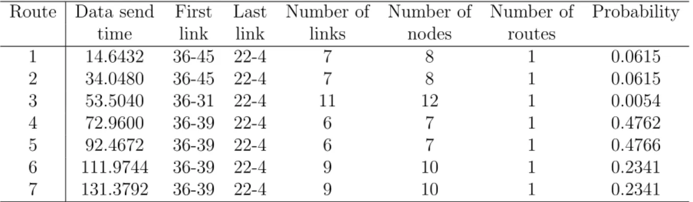
(38) Table 4.5: Results of scenario 1 using Ant Multiple Routes (AMR). Best route 4 0 0 1 1 0 0 0 0 0. Ant send First Last time link link 0.0512 36-45 22-4 14.6944 0 0 29.2864 0 0 43.8784 36-39 22-4 58.4704 36-39 22-4 73.1136 0 0 87.7568 0 0 102.4000 0 0 117.0432 0 0 131.6864 0 0. Number of links 6 0 0 6 6 0 0 0 0 0. Number of nodes 7 0 0 7 7 0 0 0 0 0. Number of routes 23 0 0 1 1 0 0 0 0 0. Probability 1 × 10−6 0.0001 0 0 0.0022 0.1385 0 0 0 0 0. Table 4.6: Not fixed parameters for scenario 2. Simulation time Node population (Ntot ) Maximum node speed (Vmax ) Beacon time (tbeacon ) Maximum transmission radius (r) Minimum received power (Pthreshold ) Ant time (tants ) Minimum pheromone. 150 sec 56 0 m/s 30 sec 18 m 4.7630 × 10−8 w 20 sec 7 units. There are 6 links and 7 nodes along the route with a probability of 0.1571. Check that using Ant Best Route (ABR), we only lost one data packet, so that we always have a route to the destination node although the packet has to go through a longer route.. 4.2.2. Scenario 2. In this scenario we employ the topology of scenario 1 but we change some parameters to analyze the behavior of the network, which are presented in Table 4.6. Table 4.7, and 4.8 show the results obtained with routing methods. Notice from Table 4.8 that some ants are getting to the destination node so we have a better behavior than in scenario 1 but it is not enough to support the routes all the time. 33.

(39) Table 4.7: Results of scenario 2 using Ant Best Route (ABR). Route 1 2 3 4 5 6 7. Data send First Last time link link 14.6432 36-45 22-4 34.0480 36-45 22-4 53.5040 36-31 22-4 72.9600 36-39 22-4 92.4672 36-39 22-4 111.9744 36-39 22-4 131.3792 36-39 22-4. Number of links 7 7 11 6 6 9 9. Number of nodes 8 8 12 7 7 10 10. Number of routes 1 1 1 1 1 1 1. Probability 0.0615 0.0615 0.0054 0.4762 0.4766 0.2341 0.2341. Table 4.8: Results of scenario 2 using Ant Multiple Routes (AMR). Best route 1 0 1 1 0 1 0. Ant send First Last time link link 0.0512 36-39 22-4 19.5072 0 0 38.9632 36-39 22-4 58.4192 36-39 22-4 77.9264 0 0 97.4336 36-39 22-4 116.9408 0 0. Number of links 6 0 6 6 0 6 0. 34. Number of nodes 7 0 7 7 0 7 0. Number of routes 28 0 2 1 0 3 0. Probability 1 × 10−5 0.0007 0 0.2031 0.1876 0 0.0340 0.

(40) Table 4.9: Not fixed parameters for scenario 3. Simulation time Node population (Ntot ) Maximum node speed (Vmax ) Beacon time (tbeacon ) Maximum transmission radius (r) Minimum received power (Pthreshold ) Ant time (tants ) Minimum pheromone. 150 sec 56 0 m/s 20 sec 18 m 4.7630 × 10−8 w 15 sec 35 units. In table 4.7 like in scenario 1 we always have a route to the destination node although the packet has to go through a long route. What we can say from the last two scenarios, the ants do not arrive at the destination node because the buffers are full in the nodes and for this reason the ants ”die” before finding the destination node. Therefore we use an equation looking for an adequate time life of the ants in the network to get a better development of the routing methods. 1 B, (4.3) λ is the time that the ant should live in the network in time units, B is the tlif eunit =. where tlif eunits. buffer size and λ is equal to λ=. α tants. ,. where α is the number of ants in the interval [0,tants ]. In the next scenarios, we use Equation (4.3) to analyze the performance of the routing methods.. 4.2.3. Scenario 3. In the present scenario, we consider Equation (4.3) in the topology of Figure 4.2. We use the same values of the parameters of scenario 1 and only change the minimum pheromone. Table 4.9 shows the parameters employed, and tables 4.10, 4.11 the results obtained. From the results in Table 4.11, we can observe that at least one ant is arriving to the destination node every time of send (tants ), so that we have a route to the destination node 35.

(41) Table 4.10: Results of scenario 3 using Ant Best Route (ABR). Route 1 2 3 4 5 6 7 8 9 10. Data send time 9.7792 24.3200 38.9120 53.5040 68.0960 82.7392 97.3312 111.9232 126.5152 141.1072. First Last link link 36-39 22-4 36-31 22-4 36-31 22-4 36-39 22-4 36-39 22-4 36-31 22-4 36-39 22-4 36-39 22-4 36-31 22-4 36-39 22-4. Number of links 6 12 12 6 6 12 6 6 11 6. Number of nodes 7 13 13 7 7 13 7 7 12 7. Number of routes 1 1 1 1 1 1 1 1 1 1. Probability 0.0954 0.0271 0.2535 0.5326 0.7596 0.3207 0.7753 0.8874 0.2143 0.7358. Table 4.11: Results of scenario 3 using Ant Multiple Routes (AMR). Best route 2 1 1 1 1 1 1 1 1 1. Ant send time 0.0512 14.6944 29.3376 43.8784 58.4704 73.1136 87.7568 102.4000 117.0432 131.6864. First Last link link 36-39 22-4 36-39 22-4 36-39 22-4 36-39 22-4 36-39 22-4 36-39 22-4 36-39 22-4 36-39 22-4 36-39 22-4 36-39 22-4. Number of links 6 6 6 6 6 6 6 6 6 6. 36. Number of nodes 7 7 7 7 7 7 7 7 7 7. Number of routes 11 5 3 1 1 4 1 1 2 1. Probability 1 × 10−5 0.0000 0.0053 0.0147 0.2186 0.1192 0.0131 0.0075 0.1256 0.1654 0.1852.

(42) Table 4.12: Not fixed parameters for scenario 4. Simulation time Node population (Ntot ) Maximum node speed (Vmax ) Beacon time (tbeacon ) Maximum transmission radius (r) Minimum received power (Pthreshold ) Ant time (tants ) Minimum pheromone. 150 sec 56 0 m/s 30 sec 18 m 4.7630 × 10−8 w 20 sec 27 units. Table 4.13: Results of scenario 4 using Ant Best Route (ABR). Route 1 2 3 4 5 6 7. Data send First Last time link link 14.6432 36-39 22-4 34.0480 36-31 22-4 53.5040 36-31 22-4 72.9600 36-39 22-4 92.4672 36-31 22-4 111.9744 36-31 22-4 131.3792 36-39 22-4. Number of links 6 15 13 6 13 13 6. Number of nodes 7 16 14 7 14 14 7. Number of routes 1 1 1 1 1 1 1. Probability 0.1419 0.0989 0.2689 0.5061 0.4231 0.5080 0.5155. every time, which could be considered the best route for Ant Multiple Routes (AMR). In Table 4.10, we always have a route to the destination node but in some cases the routes are long, that is because the ants that pass through the nodes influence in the routing decisions.. 4.2.4. Scenario 4. In this scenario, we use the same values of the parameters of scenario 2, and only change the minimum pheromone. Table 4.12 shows the parameters considered, and Tables 4.13, 4.14 the results obtained for Ant Best Route (ABR), and Ant Multiple Routes (AMR). From the last results, we can observe that the behavior of the system is more stable, and we have more routes to the destination node in Table 4.14. On the other hand, in Table 4.13 the routes to the destination node are long. Notice that applying equation 4.3 to the last two scenarios, we reduce the life time of 37.

(43) Table 4.14: Results of scenario 4 using Ant Multiple Routes (AMR). Best route 1 1 1 1 1 1 1. Ant send time 0.0512 19.5072 38.9632 58.4192 77.9264 97.4336 116.9408. First Last link link 36-39 22-4 36-39 22-4 36-39 22-4 36-39 22-4 36-39 22-4 36-39 22-4 36-39 22-4. Number of links 6 6 6 6 6 6 6. Number of nodes 7 7 7 7 7 7 7. Number of routes 14 11 5 5 5 5 5. Probability 1 × 10−4 0.0011 0.0574 0.0498 0.0318 0.0503 0.1259 0.1759. the ants (tlif eunits ), and we get a better development for Ant Multiple Routes (AMR), so that more ants are reaching the destination node. As the number of nodes increases or decreases in the network, we have to modify the time between ants (tant ) to maintain the ant life time (tlif eunits ) constant, and consequently maintain a stable behavior of the network. Figure 4.3 shows the conduct of the network for several ant life times (tlif eunits ), where we can observe the linear performance of the system. In the next scenarios, we analyze the behavior of the network for some ant life times (tlif eunits ), where there is no mobility.. 4.2.5. Scenario 5. In scenario 5, we employ a time between beacons (tbeacon ) of 10 sec, and the topology of Figure 4.2. Table 4.15 shows the parameters considered, where the ant life time (tlif eunits ) is 13 time units. Tables 4.16, and 4.17 present the results obtained for Ant Best Route (ABR), and Multiple Routes (AMR). We can observe from Table 4.16 that the number of links to get the destination node are more stable than in the last scenarios. On the other hand, in Table 4.17 there are some ants that are not reaching the destination node, also we have few routes to the destination.. 38.

(44) Table 4.15: Not fixed parameters for scenario 5. Simulation time Node population (Ntot ) Maximum node speed (Vmax ) Beacon time (tbeacon ) Maximum transmission radius (r) Minimum received power (Pthreshold ) Ant time (tants ) Minimum pheromone. 150 sec 56 0 m/s 10 sec 18 m 4.7630 × 10−8 w 10 sec 50 units. Table 4.16: Results of scenario 5 using Ant Best Route (ABR). Route 1 2 3 4 5 6 7 8 9 10 11 12 13 14 15. Data send time 6.8608 16.5888 26.2656 35.9936 45.7216 55.4496 65.1776 74.9056 84.6848 94.4128 104.1408 113.8688 123.5968 133.3248 143.0528. First Last link link 36-39 22-4 36-31 22-4 36-31 22-4 36-31 22-4 36-31 22-4 36-39 22-4 36-39 22-4 36-39 22-4 36-39 22-4 36-39 22-4 36-39 22-4 36-39 22-4 36-39 22-4 36-39 22-4 36-39 22-4. Number of links 6 9 9 9 9 9 9 9 6 8 9 9 9 6 6. 39. Number of nodes 7 10 10 10 10 10 10 10 7 9 10 10 10 7 7. Number of routes 1 1 1 1 1 1 1 1 1 1 1 1 1 1 1. Probability 0.0071 0.0454 0.0604 0.0604 0.0604 0.2416 0.2416 0.3616 0.6429 0.4874 0.4700 0.5136 0.5694 0.5960 0.5997.

(45) Figure 4.3: Behavior of the network owing to Ant Life Time.. 4.2.6. Scenario 6. In the present scenario, we maintain the topology of Figure 4.2 and only change the time between ants a 20 sec (tants ). Table 4.18 shows the parameters employed, where the ant life time (tlif eunits ) is 26 time units. Tables 4.19, and 4.20 present the results obtained. Notice from Table 4.19 that the number of links to get the destination node are more stable. On the other hand, in Table 4.20 we have many routes to the destination node. Figure 4.3 presents some graphs for various ant life times (tlif eunits ), which shows the behavior linear of the network for every value. Is important to mention that according as the ant life time (tlif eunits ) is major, more ants arrive at the destination node, and the performance of the routing methods is better, where Ant Multiple Routes (AMR) has more routes to the destination node, and Ant Best Route (ABR) has short and stable routes to the destination. Also notice that the graphs indicate that as the number of nodes change in the network, the time between ants (tant ) must to be modified to maintain the ant life time (tlif eunits ) constant, and consequently maintain a stable behavior of the network.. 40.

(46) Table 4.17: Results of scenario 5 using Ant Multiple Routes (AMR). Best route 2 2 0 0 0 1 0 0 1 1 1 1 1 1 1. Ant send time 0.0512 9.8304 19.5584 29.2864 39.0144 48.7424 58.4704 68.2496 78.0288 87.8080 97.5872 107.3664 117.1456 126.9248 136.7040. First Last link link 36-39 22-4 36-45 22-4 0 0 0 0 0 0 36-39 22-4 0 0 0 0 36-39 22-4 36-39 22-4 36-39 22-4 36-39 22-4 36-39 22-4 36-39 22-4 36-39 22-4. Number of links 6 7 0 0 0 6 0 0 6 6 6 6 6 6 6. Number of nodes 7 8 0 0 0 7 0 0 7 7 7 7 7 7 7. Number of routes 6 3 0 0 0 3 0 0 3 3 3 3 3 3 3. Table 4.18: Not fixed parameters for scenario 6. Simulation time Node population (Ntot ) Maximum node speed (Vmax ) Beacon time (tbeacon ) Maximum transmission radius (r) Minimum received power (Pthreshold ) Ant time (tants ) Minimum pheromone. 41. 150 sec 56 0 m/s 10 sec 18 m 4.7630 × 10−8 w 20 sec 26 units. Probability 1 × 10−5 0.0001 0.0370 0 0 0 0.4936 0 0 0.5542 0.5709 0.3972 0.6735 0.6109 0.4626 0.5593.

(47) Table 4.19: Results of scenario 6 using Ant Best Route (ABR). Route 1 2 3 4 5 6 7. Data send First Last time link link 14.6432 36-39 22-4 34.0480 36-45 22-4 53.5040 36-45 22-4 72.9600 36-45 22-4 92.4672 36-45 22-4 111.9744 36-39 22-4 131.3792 36-45 22-4. Number of links 7 7 7 7 7 7 8. Number of nodes 8 8 8 8 8 8 9. Number of routes 1 1 1 1 1 1 1. Probability 0.0669 0.1044 0.1632 0.1954 0.2091 0.2359 0.0789. Table 4.20: Results of scenario 6 using Ant Multiple Routes (AMR). Best route 1 1 1 1 1 1 1. Ant send time 0.0512 19.5072 38.9632 58.4192 77.9264 97.4336 116.9408. First Last link link 36-39 22-4 36-39 22-4 36-39 22-4 36-39 22-4 36-39 22-4 36-39 22-4 36-39 22-4. Number of links 6 6 6 6 6 6 6. 42. Number of nodes 7 7 7 7 7 7 7. Number of routes 14 15 15 15 15 14 15. Probability 1 × 10−6 0.0326 0.4720 0.4584 0.4730 0.4729 0.4726 0.3980.

(48) Table 4.21: Not fixed parameters for scenario 7. Simulation time Node population (Ntot ) Maximum node speed (Vmax ) Beacon time (tbeacon ) Maximum transmission radius (r) Minimum received power (Pthreshold ) Ant time (tants ) Minimum pheromone. 250 sec 56 2 m/s 5 sec 18 m 4.7630 × 10−8 w 10 sec 50 units. In the next scenarios, we analyze the conduct of the routing methods with mobility.. 4.2.7. Scenario 7. In the present scenario, we employ the topology of Figure 4.2, where half of the nodes move with a speed between [0-2] m/s, and the other half stay static (no mobility). The simulation time is about 250 sec, and the nodes located on the corners are considered service nodes, which remain static all the time. We analyze the routing behavior between the service node number 4 (position (99, 99)) and node number 36 (position (50, 50)) where node 36 is considered the source node and node 4 the destination node. Table 4.21 shows the parameters considered, where the ant life time (tlif eunits ) is 13 time units, and the time between beacons is 5 sec (tbeacons ). Tables 4.22, and 4.23 present the results obtained for Ant Best Route (ABR), and Ant Multiple Routes (AMR). Notice from Table 4.23 that using Ant Multiple Routes (AMR), we always have routes to the destination node every time. On the other hand, using Ant Best Route (ABR) not all the data packets are reaching the destination, and consequently we do not have a good route to it every time.. 4.2.8. Scenario 8. In this scenario, we use the same values of the parameters of scenario 7, and only change the time between ants a 15 sec (tants ). Table 4.24 shows the parameters considered, where the ant life time (tlif eunits ) is 20 time units. Tables 4.25, and 4.26 present the results obtained for Ant Best Route (ABR), and Ant Multiple Routes (AMR).. 43.

(49) Table 4.22: Results of scenario 7 using Ant Best Route (ABR). Route 1 2 3 4 5 6 7 8 9 10 11 12 13 14 15 16 17 18 19 20 21 22 23 24. Data send time 7.0000 16.2656 26.2656 35.9936 45.9936 55.4496 64.9056 74.9056 84.6848 94.4128 113.5968 123.5968 133.3248 143.0528 152.7808 162.7808 171.7808 181.7808 191.7808 201.7808 211.7808 220.7808 230.3328 240.3328. First Last link link 0 0 0 0 36-55 22-4 36-25 22-4 0 0 36-30 22-4 0 0 36-19 22-4 36-19 22-4 36-43 22-4 0 0 36-43 22-4 36-43 22-4 36-55 53-4 36-53 53-4 0 0 0 0 0 0 0 0 0 0 0 0 0 0 0 0 36-40 22-4. Number of links 0 0 7 6 0 6 0 3 3 4 0 5 5 3 2 0 0 0 0 0 0 0 0 7. 44. Number of nodes 0 0 8 7 0 7 0 4 4 5 0 6 6 4 3 0 0 0 0 0 0 0 0 8. Number of routes 0 0 1 1 0 1 0 1 1 1 0 1 1 1 1 0 0 0 0 0 0 0 0 1. Probability 0 0 0.1071 0.2351 0 0.2865 0 0.2268 0.2132 0.2092 0 0.1959 0.0834 0.1227 0.3125 0 0 0 0 0 0 0 0 0.2564.

(50) Table 4.23: Results of scenario 7 using Ant Multiple Routes (AMR). Best route 1 2 2 1 1 2 1 2 2 6 5 1 1 1 1 1 1 1 1 1 0 1 1 1 1. Ant send time 0.0512 9.8304 19.5584 29.2864 39.0144 48.7424 58.4704 68.2496 78.0288 87.8080 97.5872 107.3664 117.1456 126.9248 136.7040 146.4832 156.2624 166.0416 175.8208 185.6000 195.3792 205.1584 214.9376 224.7168 234.4960. First Last link link 36-39 22-4 36-46 22-4 36-25 22-4 36-25 22-4 36-25 22-4 36-30 22-4 36-8 50-4 36-19 39-4 36-19 34-4 36-19 22-4 36-34 22-4 36-19 22-4 36-22 22-4 36-22 22-4 36-4 36-4 36-4 36-4 36-4 36-4 36-4 36-4 36-4 36-4 36-42 42-4 0 0 36-51 33-4 36-46 33-4 36-13 22-4 36-40 22-4. Number of links 6 5 5 5 6 5 4 3 3 4 3 3 2 2 1 1 1 1 1 2 0 3 3 7 6. Number of nodes 7 6 6 6 7 6 5 4 4 5 4 4 3 3 2 2 2 2 2 3 0 4 4 8 7. Number of routes 3 7 5 6 8 5 8 11 10 9 5 5 6 7 5 2 10 3 10 9 0 3 6 4 4. Table 4.24: Not fixed parameters for scenario 8. Simulation time Node population (Ntot ) Maximum node speed (Vmax ) Beacon time (tbeacon ) Maximum transmission radius (r) Minimum received power (Pthreshold ) Ant time (tants ) Minimum pheromone. 45. 250 sec 56 2 m/s 5 sec 18 m 4.7630 × 10−8 w 15 sec 35 units. Probability 0.0000 0.0000 0.0000 0.0000 0.0000 0.0000 0.0025 0.0023 0.0025 0.0000 0.0001 0.0002 0.0007 0.0118 0.4057 0.4919 0.5069 0.4717 0.0897 0.0864 0 0.0433 0.0127 0.0000 0.0000.

(51) Table 4.25: Results of scenario 8 using Ant Best Route (ABR). Route 1 2 3 4 5 6 7 8 9 10 11 12 13 14 15 16 17. Data send First Last time link link 9.7792 36-45 22-4 24.3200 36-45 22-4 38.9120 0 0 53.5040 0 0 68.0960 36-52 22-4 82.7392 36-11 22-4 97.3312 0 0 111.9232 0 0 126.5152 0 0 141.1072 36-11 22-4 155.6992 36-52 22-4 170.6992 0 0 184.6992 0 0 200.1072 0 0 215.9232 0 0 229.5252 0 0 245.5040 0 0. Number of links 6 7 0 0 7 7 0 0 0 7 6 0 0 0 0 0 0. 46. Number of nodes 7 8 0 0 8 8 0 0 0 8 7 0 0 0 0 0 0. Number of routes 1 1 0 0 1 1 0 0 0 1 1 0 0 0 0 0 0. Probability 0.0067 0.1434 0 0 0.1533 0.2260 0 0 0 0.3840 0.2281 0 0 0 0 0 0.

(52) Table 4.26: Results of scenario 8 using Ant Multiple Routes (AMR). Best route 1 1 1 0 2 2 1 1 2 3 1 1 0 0 1 0 0. Ant send time 0.0512 14.6944 29.3376 43.8784 58.4704 73.1136 87.7568 102.4000 117.0432 131.6864 146.4832 161.1264 175.7696 190.4128 205.0560 219.6992 234.3424. First Last link link 36-39 22-4 36-45 22-4 36-44 22-4 0 0 36-52 22-4 36-11 22-4 36-11 22-4 36-11 32-4 36-11 32-4 36-11 22-4 36-52 22-4 36-52 22-4 0 0 0 0 36-37 34-4 0 0 0 0. Number of links 7 6 7 0 6 7 7 8 7 7 6 6 0 0 7 0 0. 47. Number of nodes 8 7 8 0 7 8 8 9 8 8 7 7 0 0 8 0 0. Number of routes 3 4 2 0 4 4 8 2 11 10 7 5 0 0 3 0 0. Probability 1 × 10−4 0.0000 0.0000 0.0000 0 0.0000 0.0000 0.0000 0.0000 0.0000 0.0000 0.0013 0.0000 0 0 0.4377 0 0.

(53) Observe that using Ant Multiple Routes (AMR), we have almost all time a routes to the destination node. Using Ant Best Route (ABR) not all the data packets are getting the destination. Notice in the scenarios where we apply Equation 4.3 (scenarios 3 to 8) that the number of nodes to arrive at the destination node using Ant Multiple Routes (AMR) is less or equal to the ant life time (tlif eunits ) in each case. This indicate us that the ant life time (tlif eunits ) in each scenario is adequate, so that the ants get the destination and give us the best routes to it since the ants that take the saturated or long routes die in the way. For the next set of figures we choose the topology of Figure 4.2, and we analyze the throughput for Ant Best Route (ABR) between the service node number 4 (position (99, 99)) and node number 36 (position (50, 50)), where node 36 is considered the source node and node 4 the destination node. The simulation time is about 250 sec, and half of the nodes move with a speed between [0-2] m/s, and the other half stay static (no mobility). Figure 4.4 shows the average number of data packets received at the destination node per packet sent by the source node for some ant times (tants ). Notice that the number of packets received in the destination decrease when the beacon time (tbeacon ) increase. By the other hand Figure 4.5 illustrate the average number of data packets received by the destination node per simulation time. Figures 4.6, and 4.8 present the average number of data packets received at the destination node per packet sent by the source node for some ant life time (tlif eunits ) in pheromone units. The maximum points of the graphics correspond to the best performance of the method, which are getting when there is an adequate time life of the ants in the network according Equation 4.3. Also notice that Figure 4.3 shows the conduct of the network for several ant life times (tlif eunits ), and from Figures 4.6, and 4.8, we can observe that under mobility an ant life time (tlif eunits ) of 13 time units or 50 pheromone units could be an adequate value for the network. Figure 4.6 shows the graphics for a beacon time (tbeacon ) of 5 sec and Figure 4.8 for 10 sec. Figures 4.7 and 4.9 illustrate the average number of data packets received at the destination node per simulation time.. 48.

(54) Figure 4.4: Packets delivered (pkts received/pkts sent) for Ant Best Route (ABR) with a Vmax =2m/s.. Figure 4.5: Packets delivered (pkts received/simulation time) for Ant Best Route (ABR) with a Vmax =2m/s. 49.

(55) Figure 4.6: Packets delivered (pkts received/pkts sent) for Ant Best Route (ABR) with a tbeacon =5sec, and Vmax =2 m/s.. Figure 4.7: Packets delivered (pkts received/simulation time) for Ant Best Route (ABR) with a tbeacon =5sec, and Vmax =2 m/s. 50.

(56) Figure 4.8: Packets delivered (pkts received/pkts sent) for Ant Best Route (ABR) with a tbeacon =10sec, and Vmax =2 m/s.. Figure 4.9: Packets delivered (pkts received/simulation time) for Ant Best Route (ABR) with a tbeacon =10sec, and Vmax =2 m/s. 51.