Performance Analysis of the IEEE 802 11 CSMA/CA for the transmission of VoWLAN under high interference scenarios Edición Única

Texto completo

(1)INSTITUTO TECNOLÓGICO Y DE ESTUDIOS SUPERIORES DE MONTERREY Campus Monterrey. PROGRAMA DE GRADUADOS DE LA DIVISIÓN DE TECNOLOGÍAS DE INFORMACION Y ELECTRÓNICA. Performance Analysis of the IEEE 802.11 CSMA/CA for the transmission of VoWLAN under high interference scenarios THESIS PRESENTED IN PARTIAL FULFILLMENT OF THE REQUIREMENTS FOR THE DEGREE OF MASTER OF SCIENCE IN ELECTRONICS ENGINEERING WITH MAJOR IN TELECOMMUNICATIONS BY. Alberto Jorge Hernández Estala. Monterrey, N.L. November, 2005.

(2) INSTITUTO TECNOLÓGICO Y DE ESTUDIOS SUPERIORES DE MONTERREY Campus Monterrey. PROGRAMA DE GRADUADOS DE LA DIVISIÓN DE TECNOLOGÍAS DE INFORMACION Y ELECTRÓNICA. Performance Analysis of the IEEE 802.11 CSMA/CA for the transmission of VoWLAN under high interference scenarios THESIS PRESENTED IN PARTIAL FULFILLMENT OF THE REQUIREMENTS FOR THE DEGREE OF MASTER OF SCIENCE IN ELECTRONICS ENGINEERING WITH MAJOR IN TELECOMMUNICATIONS BY. Alberto Jorge Hernández Estala. Monterrey, N.L. November, 2005.

(3) © Alberto Jorge Hernández Estala, 2005.

(4) INSTITUTO TECNOLÓGICO Y DE ESTUDIOS SUPERIORES DE MONTERREY Campus Monterrey PROGRAMA DE GRADUADOS DE LA DIVISIÓN DE TECNOLOGÍAS DE INFORMACION Y ELECTRÓNICA The members of the evaluation committee hereby recommend accepting the thesis presented by Alberto Jorge Hernández Estala in partial fulfillment of the requirements for the degree of Master of Science in Electronics Engineering with major in Telecommunications Thesis Committee. _____________________ Dr. David Muñoz Rodríguez Thesis Advisor. _____________________ Dr. José Ramón Rodríguez Cruz. _____________________ Dr. César Vargas Rosales. Synodal. Synodal. _____________________ Dr. David Garza Salazar Director of the Graduate Program November 2005.

(5) To my parents, Alberto and Isela For giving me their never-ending love and support. To my brothers, Ivan and Marcela For always being with me.. V.

(6) Acknowledgements First of all I want to thank my father and mother for all their unconditional support, motivation, orientation, guidance, patience and love. I also want to thank my brother and sister for being with me all the time, for the patience and love. To all my family for motivating me to never give up and accomplish all my goals and dreams. I want to thank the Instituto Tecnológico y de Estudios Superiores de Monterrey for giving me the opportunity to realize my graduate studies in this city. I want to express my gratitude to my thesis advisor, Ph.D. David Muñoz Rodríguez, for all the support given to make this work possible and for all the enriched sessions in which I learn invaluable lessons, including lessons for life. His knowledge and experience played an important role in the development of this thesis. I also want to thank Ph.D. José Ramón Rodríguez Cruz and Ph.D. César Vargas Rosales, for all their valuable comments, ideas and support to improve and conclude this work. I want to thank my friend Tamara Caballero for her motivation, support and patience during my graduate studies, and for showing me no to take life so seriously. Also, to my friends of the CET, Hugo, Marco, Mario, Michel, Hilda, Javier, Juan Carlos, Rolando and all the persons who gave me their support during this period of my life.. Alberto Jorge Hernández Estala. Instituto Tecnológico y de Estudios Superiores de Monterrey November 2005 VI.

(7) Abstract Wireless LAN technologies are becoming increasingly important and the IEEE 802.11 standard is the most mature wireless technology for data transmission throughout the Internet. It is based on the CSMA/CA protocol and provides Internet access to each station throughout a common shared medium, the air. Recently, with the rising popularity of delay sensitive applications such as Voice over Internet Protocol (VoIP) via a wireless local area network, the IEEE 802.11 is poised to become an important low cost voice transfer solution. In this thesis, we investigate the performance of the IEEE 802.11 Distributed Coordination Function in terms of the voice packets average delay experienced by the stations and the system throughput. We determine the situations and the required scenarios for the transmission of voice over WLAN under the presence of Rayleigh fading, near/far effect and co-channel interference. We also identify the required scenarios for the transmission of voice over WLAN in terms of the number of stations, its spatial distribution and we determine the maximum number of non desired overlapping cells in the same frequency band that a WLAN system can tolerate for the transmission of VoWLAN. Finally, for theoretical optimal VoWLAN transmission scenarios, the cumulative distribution function of the voice packet delay is given in terms of the number of stations, with the objective of having a quality measure for the voice transmission throughout the WLAN.. VII.

(8) Resumen Las tecnologías inalámbricas de redes de área local (LAN) son cada vez más importantes y el estándar IEEE 802.11 es la tecnología inalámbrica mas madura para la transmisión de datos a través del Internet. El estándar se basa en el protocolo CSMA/CA y proporciona una conexión a Internet utilizando un medio compartido por todas las estaciones, el aire. Actualmente, con la creciente popularidad de aplicaciones sensibles a los retrasos en la transmisión, tales como Voz sobre IP a través de una red inalámbrica, el estándar IEEE 802.22 se perfila para ser una solución de bajo costo para la transmisión de voz. En esta tesis se investiga el desempeño de la Distributed Coordination Function (DCT) del estándar IEEE 802.11 en términos del retraso de paquetes de voz en las estaciones y del throughput del canal. De manera que se determinan las situaciones y los escenarios requeridos para la transmisión de voz sobre una red inalámbrica de área local (VoWLAN); bajo la influencia de desvanecimiento tipo Rayleihg, el efecto near/far e interferencia co-canal. También se identifican los escenarios requeridos para la transmisión de voz a través de una WLAN en función del número de estaciones, su distribución espacial y se determina el número máximo tolerable de celdas traslapadas no deseadas funcionando en la misma banda de frecuencia, para poder transmitir VoWLAN. Finalmente, para los escenarios teóricamente óptimos para transmitir voz, se obtiene la función de distribución acumulativa del retraso en los paquetes de voz dada en términos del número de estaciones, con el objetivo de tener una medida de calidad para su transmisión a través de la WLAN.. VIII.

(9) Contents Acknowledgments. VI. Abstract. VII. List of Figures. XII. List of Tables. XIII. Chapter 1. Introduction 1.1 Objective 1.2 Justification 1.3 Contribution 1.4 Hypothesis. 1 2 2 3 4. Chapter 2. Fundamentals of Wireless Local Area Networks 2.1 Classification of Channel Access 2.2 Demands of transfer networks 2.2.1 Traffic Types 2.2.2 Transfer Speed 2.3 Special features of wireless networks 2.3.1 Wireless networks use a common medium 2.3.2 Spatial Characteristics 2.4 Frequency allocations 2.5 The IEEE 802.11 standard 2.5.1 Channel Access 2.5.2 IEEE 802.11 Frequency allocations. 5 5 6 6 7 7 7 7 8 9 11 21. Chapter 3. Mobile Radio Propagation 3.1 Introduction to Radio Wave Propagation 3.2 Free Space Propagation Model 3.3 Small-Scale Fading and Multipath 3.3.1 Rayleigh Distribution. 25 25 26 27 28. Chapter 4. Capture Effect in Wireless Systems under Rayleigh Fading 4.1 Capture Model under Rayleigh Fading. 30 30. Chapter 5. Saturation Throughput and Expected Delay under Co-Channel Interference 5.1 The System Model 5.1.1 Packet Transmission Probability 5.1.2 Calculation of p , pb and τ in one WLAN cell under ideal channel conditions. IX. 39 39 40 47.

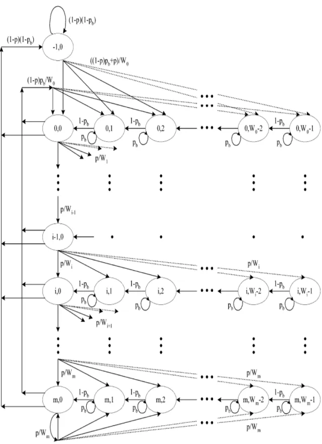
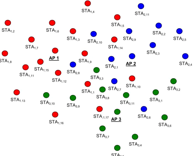
(10) 5.1.3 Calculation of p , pb and τ for any given station under Rayleigh Fading and Co-Channel Interference in a multicell IEEE 802.11 wireless system. 5.2 Saturation Throughput Analysis 5.2.1 Saturation Throughput for ideal channel conditions 5.2.2 Saturation Throughput under Rayleigh fading channels 5.2.3 Saturation Throughput under Rayleigh fading channels and the Capture Effect 5.3 Delay Analysis 5.3.1 Delay analysis on ideal channel conditions 5.3.2 Delay analysis on Rayleigh fading channels. 49 57 57 60 63 65 65 66. Chapter 6. Voice Over 802.11 6.1 Background on Voice over Internet Protocol 6.2 Interference Issues and QoS on Vo802.11 Wireless Networks 6.3 Importance of QoS on 802.11 Networks 6.4 Latency in Wireless Networks 6.5 QoS on Vo802.11 Networks 6.5.1 Measuring voice quality in Vo802.11 6.5.2 Detractors on Voice Quality in Vo802.11 Networks. 69 69 70 70 71 72 72 72. Chapter 7. Numerical Results 7.1 WLAN Scenario 1: One WLAN with a finite number of stations 7.1.1 Scenario: Signal to Noise Ratio = 6 dB at 5.5 Mbps 7.1.2 Scenario: Signal to Noise Ratio = 6 dB at 11 Mbps 7.1.3 Scenario: Signal to Noise Ratio = 6 dB at 54 Mbps 7.1.4 Scenario: Signal to Noise Ratio = 8 dB at 5.5 Mbps 7.1.5 Scenario: Signal to Noise Ratio = 8 dB at 11 Mbps 7.1.6 Scenario: Signal to Noise Ratio = 8 dB at 54 Mbps 7.1.7 Scenario: Signal to Noise Ratio = 10 dB at 5.5 Mbps 7.1.8 Scenario: Signal to Noise Ratio = 10 dB at 11 Mbps 7.1.9 Scenario: Signal to Noise Ratio = 10 dB at 54 Mbps 7.1.10 Optimal scenarios for the transmission of VoWLAN (when there are no other interfering WLANs) 7.2 WLAN scenario 2: One WLAN with a finite number of stations surrounded by other interfering WLAN’s 7.2.1. Interference Scenario 1: 5 Stations for each WLAN, SNR = 6 dB for all the WLAN’s, all WLAN’s at 54 Mbps, all WLAN’s with BAS mechanism, R1 = 20 meters and R2 variable. 76. X. 76 78 86 94 101 108 114 122 130 136 143 174. 175.

(11) 7.2.2. Interference Scenario 2: 5 Stations for each WLAN, SNR = 8 dB for all the WLAN’s, all WLAN’s at 54 Mbps, all WLAN’s with BAS mechanism, R1 = 20 meters and R2 variable 7.2.3. Interference Scenario 3: 5 Stations for each WLAN, SNR = 10 dB for all the WLAN’s, all WLAN’s at 54 Mbps, all WLAN’s with BAS mechanism, R1 = 20 meters and R2 variable 7.2.4. Interference Scenario 4: 6 Stations for each WLAN, SNR = 6 dB for all the WLAN’s, all WLAN’s at 54 Mbps, all WLAN’s with BAS mechanism, R1 = 20 meters and R2 variable 7.2.5. Interference Scenario 5: 6 Stations for each WLAN, SNR = 8 dB for all the WLAN’s, all WLAN’s at 54 Mbps, all WLAN’s with BAS mechanism, R1 = 20 meters and R2 variable 7.2.6. Interference Scenario 6: 6 Stations for each WLAN, SNR = 10 dB for all the WLAN’s, all WLAN’s at 54 Mbps, all WLAN’s with BAS mechanism, R1 = 20 meters and R2 variable 7.2.7. Interference Scenario 7: 7 Stations for each WLAN, SNR = 6 dB for all the WLAN’s, all WLAN’s at 54 Mbps, all WLAN’s with BAS mechanism, R1 = 20 meters and R2 variable 7.2.8. Interference Scenario 8: 7 Stations for each WLAN, SNR = 8 dB for all the WLAN’s, all WLAN’s at 54 Mbps, all WLAN’s with BAS mechanism, R1 = 20 meters and R2 variable 7.2.9. Interference Scenario 9: 7 Stations for each WLAN, SNR = 10 dB for all the WLAN’s, all WLAN’s at 54 Mbps, all WLAN’s with BAS mechanism, R1 = 20 meters and R2 variable. 176. 178. 179. 180. 181. 183. 184. 185. Chapter 8. Conclusions and Further Research 8.1 Conclusions 8.2 Further Research. 187 187 188. Bibliography. 189. Vita. 191. XI.

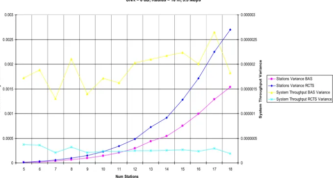
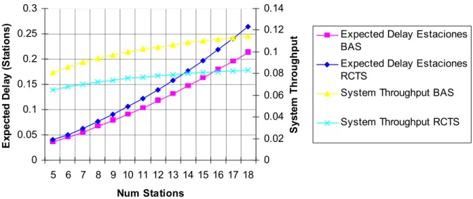
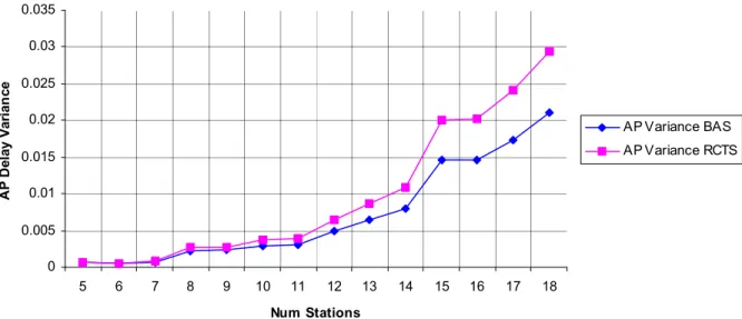
(12) List of Figures 2.1. 2.2. 2.3. 2.4. 2.5. 2.6. 2.7. 2.8. 2.9. 2.10. 2.11. 2.12. 2.13. 2.14. 2.15.. Components of an IEEE 802.11 WLAN System IEEE 802.11 and the OSI model Basic Channel Access Method Basic Service Set, showing the Hidden Node Problem Channel Access using RTS/CST IEEE 802.11 Contention Window Exponential Backoff Flowchart of the process of sending data packets under CSMA/CA RTS-CTS Access Mechanism Using the NAV in RTS-CTS Using the Backoff Counter in RTS-CTS Access Mechanism Decrementing the Backoff Counter in RTS-CTS Access Mechanism Suffering a collision in RTS-CTS Access Mechanism Channel Assignment in IEEE 802.11b Specification of the U-NII 5 GHz There are 8 non-overlapping channels in IEEE 802.11a. 9 11 13 14 15 17 19 20 20 20 21 22 23 23 24. 5.1. 5.2. 5.3.. The state transition diagram for the Markov chain model An IEEE 802.11 WLAN with a fixed number of stations η Three IEEE 802.11 WLANs operating in the same frequency band, making a total of η stations.. 42 48. Access Point Expected Delay for SNR = 6 dB, Radius = 10 m, Bit Rate = 5.5 Mbps 7.2. Stations Expected Delay and System Throughput for SNR = 6 dB, Radius = 10 m, at 5.5 Mbps 7.3. AP Delay Variance for SNR = 6 dB, Radius = 10 m, at 5.5 Mbps 7.4. Stations Delay Variance and System Throughput Variance for SNR = 6 dB, Radius = 10 m, at 5.5 Mbps 7.5. Access Point Expected Delay for SNR = 6 dB, Radius = 20 m, Bit Rate = 5.5 Mbps 7.6. Stations Expected Delay and System Throughput for SNR = 6 dB, Radius = 20 m, Bit Rate = 5.5 Mbps 7.7. AP Delay Variance for SNR = 6 dB, Radius = 20 m, Bit Rate = 5.5 Mbps 7.8. Stations Delay Variance and System Throughput Variance for SNR = 6 dB, Radius = 20 m, Bit Rate = 5.5 Mbps 7.9. AP Expected Delay for SNR = 6 dB, Radius = 30 m, Bit Rate = 5.5 Mbps 7.10. Stations Expected Delay and System Throughput for SNR = 6 dB, Radius = 30 m, Bit Rate = 5.5 Mbps. 50. 7.1.. XII. 78 79 80 81 82 82 83 84 84 85.

(13) 7.11. AP Delay Variance for SNR = 6 dB, Radius = 30 m, Bit Rate = 5.5 Mbps 7.12. Stations Delay Variance and System Throughput Variance for SNR = 6 dB, Radius = 30 m, Bit Rate = 5.5 Mbps 7.13. AP Expected Delay for SNR = 6 dB, Radius = 10 m, Bit Rate = 11 Mbps 7.14. Stations Expected Delay and System Throughput for SNR = 6 dB, Radius = 10 m, Bit Rate = 11 Mbps 7.15. AP Delay Variance for SNR = 6 dB, Radius = 10 m, Bit Rate = 11 Mbps 7.16. Stations Delay Variance and System Throughput Variance for SNR = 6 dB, Radius = 10 m, Bit Rate = 11 Mbps 7.17. AP Expected Delay for SNR = 6 dB, Radius = 20 m, Bit Rate = 11 Mbps 7.18. Stations Expected Delay and System Throughput for SNR = 6 dB, Radius = 20 m, Bit Rate = 11 Mbps 7.19. AP Delay Variance for SNR = 6 dB, Radius = 20 m, Bit Rate = 11 Mbps 7.20. Stations Delay Variance and System Throughput Variance for SNR = 6 dB, Radius = 20 m, Bit Rate = 11 Mbps 7.21. AP Expected Delay for SNR = 6 dB, Radius = 30 m, Bit Rate = 11 Mbps 7.22. Stations Expected Delay and System Throughput for SNR = 6 dB, Radius = 30 m, Bit Rate = 11 Mbps 7.23. AP Delay Variance for SNR = 6 dB, Radius = 30 m, Bit Rate = 11 Mbps 7.24. Stations Delay Variance and System Throughput Variance for SNR = 6 dB, Radius = 30 m, Bit Rate = 11 Mbps 7.25. AP Expected Delay for SNR = 6 dB, Radius = 10 m, Bit Rate = 54 Mbps 7.26. Stations Expected Delay and System Throughput for SNR = 6 dB, Radius = 10 m, Bit Rate = 54 Mbps 7.27. AP Delay Variance for SNR = 6 dB, Radius = 10 m, Bit Rate = 54 Mbps 7.28. Stations Delay Variance and System Throughput Variance for SNR = 6 dB, Radius = 10 m, Bit Rate = 54 Mbps 7.29. AP Expected Delay for SNR = 6 dB, Radius = 20 m, Bit Rate = 54 Mbps 7.30. Stations Expected Delay and System Throughput for SNR = 6 dB, Radius = 20 m, Bit Rate = 54 Mbps 7.31. AP Delay Variance for SNR = 6 dB, Radius = 20 m, Bit Rate = 54 Mbps 7.32. Stations Delay Variance and System Throughput Variance for SNR = 6 dB, Radius = 20 m, Bit Rate = 54 Mbps 7.33. AP Expected Delay for SNR = 6 dB, Radius = 30 m, Bit Rate = 54 Mbps XIII. 86 86 87 87 88 89 89 90 90 91 92 92 93 93 94 94 95 95 97 97 98 98 99.

(14) 7.34. Stations Expected Delay and System Throughput for SNR = 6 dB, Radius = 30 m, Bit Rate = 54 Mbps 7.35. AP Delay Variance for SNR = 6 dB, Radius = 30 m, Bit Rate = 54 Mbps 7.36. Stations Delay Variance and System Throughput Variance for SNR = 6 dB, Radius = 30 m, Bit Rate = 54 Mbps 7.37. AP Expected Delay for SNR = 8 dB, Radius = 10 m, Bit Rate = 5.5 Mbps 7.38. Stations Expected Delay and System Throughput for SNR = 8 dB, Radius = 10 m, Bit Rate = 5.5 Mbps 7.39. AP Delay Variance for SNR = 8 dB, Radius = 10 m, Bit Rate = 5.5 Mbps 7.40. Stations Delay Variance and System Throughput Variance for SNR = 8 dB, Radius = 10 m, Bit Rate = 54 Mbps 7.41. AP Expected Delay for SNR = 8 dB, Radius = 20 m, Bit Rate = 5.5 Mbps 7.42. Stations Expected Delay and System Throughput for SNR = 8 dB, Radius = 20 m, Bit Rate = 5.5 Mbps 7.43. AP Delay Variance for SNR = 8 dB, Radius = 20 m, Bit Rate = 5.5 Mbps 7.44. Stations Delay Variance and System Throughput Variance for SNR = 8 dB, Radius = 20 m, Bit Rate = 5.5 Mbps 7.45. AP Expected Delay for SNR = 8 dB, Radius = 30 m, Bit Rate = 5.5 Mbps 7.46. Stations Expected Delay and System Throughput for SNR = 8 dB, Radius = 30 m, Bit Rate = 5.5 Mbps 7.47. AP Delay Variance for SNR = 8 dB, Radius = 30 m, Bit Rate = 5.5 Mbps 7.48. Stations Delay Variance and System Throughput Variance for SNR = 8 dB, Radius = 30 m, Bit Rate = 5.5 Mbps 7.49. AP Expected Delay for SNR = 8 dB, Radius = 10 m, Bit Rate = 11 Mbps 7.50. Stations Expected Delay and System Throughput for SNR = 8 dB, Radius = 10 m, Bit Rate = 11 Mbps 7.51. AP Delay Variance for SNR = 8 dB, Radius = 10 m, Bit Rate = 11 Mbps 7.52. Stations Delay Variance and System Throughput Variance for SNR = 8 dB, Radius = 10 m, Bit Rate = 11 Mbps 7.53. AP Expected Delay for SNR = 8 dB, Radius = 20 m, Bit Rate = 11 Mbps 7.54. Stations Expected Delay and System Throughput for SNR = 8 dB, Radius = 20 m, Bit Rate = 11 Mbps 7.55. AP Delay Variance for SNR = 8 dB, Radius = 20 m, Bit Rate = 11 Mbps 7.56. Stations Delay Variance and System Throughput Variance for SNR = 8 dB, Radius = 20 m, Bit Rate = 11 Mbps XIV. 99 100 100 102 102 103 103 104 104 105 105 106 107 107 108 109 109 110 110 111 111 112 112.

(15) 7.57. AP Expected Delay for SNR = 8 dB, Radius = 30 m, Bit Rate = 11 Mbps 7.58. Stations Expected Delay and System Throughput for SNR = 8 dB, Radius = 30 m, Bit Rate = 11 Mbps 7.59. AP Delay Variance for SNR = 8 dB, Radius = 20 m, Bit Rate = 11 Mbps 7.60. Stations Delay Variance and System Throughput Variance for SNR = 8 dB, Radius = 20 m, Bit Rate = 11 Mbps 7.61. AP Expected Delay for SNR = 8 dB, Radius = 10 m, Bit Rate = 54 Mbps 7.62. Stations Expected Delay and System Throughput for SNR = 8 dB, Radius = 10 m, Bit Rate = 54 Mbps 7.63. AP Delay Variance for SNR = 8 dB, Radius = 10 m, Bit Rate = 54 Mbps 7.64. Stations Delay Variance and System Throughput Variance for SNR = 8 dB, Radius = 10 m, Bit Rate = 54 Mbps 7.65. AP Expected Delay for SNR = 8 dB, Radius = 20 m, Bit Rate = 54 Mbps 7.66. Stations Expected Delay and System Throughput for SNR = 8 dB, Radius = 20 m, Bit Rate = 54 Mbps 7.67. AP Delay Variance for SNR = 8 dB, Radius = 20 m, Bit Rate = 54 Mbps 7.68. Stations Delay Variance and System Throughput Variance for SNR = 8 dB, Radius = 20 m, Bit Rate = 54 Mbps 7.69. AP Expected Delay for SNR = 8 dB, Radius = 30 m, Bit Rate = 54 Mbps 7.70. Stations Expected Delay and System Throughput for SNR = 8 dB, Radius = 30 m, Bit Rate = 54 Mbps 7.71. AP Delay Variance for SNR = 8 dB, Radius = 30 m, Bit Rate = 54 Mbps 7.72. Stations Delay Variance and System Throughput Variance for SNR = 8 dB, Radius = 30 m, Bit Rate = 54 Mbps 7.73. AP Expected Delay for SNR = 10 dB, Radius = 10 m, Bit Rate = 5.5 Mbps 7.74. Stations Expected Delay and System Throughput for SNR = 10 dB, Radius = 10 m, Bit Rate = 5.5 Mbps 7.75. AP Delay Variance for SNR = 10 dB, Radius = 10 m, Bit Rate = 5.5 Mbps 7.76. Stations Delay Variance and System Throughput Variance for SNR = 10 dB, Radius = 10 m, Bit Rate = 5.5 Mbps 7.77. AP Expected Delay for SNR = 10 dB, Radius = 20 m, Bit Rate = 5.5 Mbps 7.78. Stations Expected Delay and System Throughput for SNR = 10 dB, Radius = 20 m, Bit Rate = 5.5 Mbps 7.79. AP Delay Variance for SNR = 10 dB, Radius = 10 m, Bit Rate = 5.5 Mbps XV. 113 113 114 114 115 115 116 116 117 118 118 119 120 120 121 121 122 123 123 124 125 125 126.

(16) 7.80. Stations Delay Variance and System Throughput Variance for SNR = 10 dB, Radius = 10 m, Bit Rate = 5.5 Mbps 7.81. AP Expected Delay for SNR = 10 dB, Radius = 30 m, Bit Rate = 5.5 Mbps 7.82. Stations Expected Delay and System Throughput for SNR = 10 dB, Radius = 30 m, Bit Rate = 5.5 Mbps 7.83. AP Delay Variance for SNR = 10 dB, Radius = 30 m, Bit Rate = 5.5 Mbps 7.84. Stations Delay Variance and System Throughput Variance for SNR = 10 dB, Radius = 30 m, Bit Rate = 5.5 Mbps 7.85. AP Expected Delay for SNR = 10 dB, Radius = 10 m, Bit Rate = 11 Mbps 7.86. Stations Expected Delay and System Throughput for SNR = 10 dB, Radius = 30 m, Bit Rate = 5.5 Mbps 7.87. AP Delay Variance for SNR = 10 dB, Radius = 10 m, Bit Rate = 11 Mbps 7.88. Stations Delay Variance and System Throughput Variance for SNR = 10 dB, Radius = 10 m, Bit Rate = 11 Mbps 7.89. AP Expected Delay for SNR = 10 dB, Radius = 20 m, Bit Rate = 11 Mbps 7.90. Stations Expected Delay and System Throughput for SNR = 10 dB, Radius = 20 m, Bit Rate = 11 Mbps 7.91. AP Delay Variance for SNR = 10 dB, Radius = 20 m, Bit Rate = 11 Mbps 7.92. Stations Delay Variance and System Throughput Variance for SNR = 10 dB, Radius = 20 m, Bit Rate = 11 Mbps 7.93. AP Expected Delay for SNR = 10 dB, Radius = 30 m, Bit Rate = 11 Mbps 7.94. Figure 7.94. Stations Expected Delay and System Throughput for SNR = 10 dB, Radius = 30 m, Bit Rate = 11 Mbps 7.95. AP Delay Variance for SNR = 10 dB, Radius = 30 m, Bit Rate = 11 Mbps 7.96. Stations Delay Variance and System Throughput Variance for SNR = 10 dB, Radius = 30 m, Bit Rate = 11 Mbps 7.97. AP Expected Delay for SNR = 10 dB, Radius = 10 m, Bit Rate = 54 Mbps 7.98. Stations Expected Delay and System Throughput for SNR = 10 dB, Radius = 10 m, Bit Rate = 54 Mbps 7.99. AP Delay Variance for SNR = 10 dB, Radius = 10 m, Bit Rate = 54 Mbps 7.100. Stations Delay Variance and System Throughput Variance for SNR = 10 dB, Radius = 10 m, Bit Rate = 54 Mbps 7.101. AP Expected Delay for SNR = 10 dB, Radius = 20 m, Bit Rate = 54 Mbps 7.102. Stations Expected Delay and System Throughput for SNR = 10 dB, Radius = 20 m, Bit Rate = 54 Mbps XVI. 126 127 128 128 129 130 130 131 131 132 132 135 135 134 134 135 135 136 137 137 138 138 139.

(17) 7.103. AP Delay Variance for SNR = 10 dB, Radius = 20 m, Bit Rate = 54 Mbps 7.104. Stations Delay Variance and System Throughput Variance for SNR = 10 dB, Radius = 20 m, Bit Rate = 54 Mbps 7.105. AP Expected Delay for SNR = 10 dB, Radius = 30 m, Bit Rate = 54 Mbps 7.106. Stations Expected Delay and System Throughput for SNR = 10 dB, Radius = 30 m, Bit Rate = 54 Mbps 7.107. AP Delay Variance for SNR = 10 dB, Radius = 30 m, Bit Rate = 54 Mbps 7.108. Stations Delay Variance and System Throughput Variance for SNR = 10 dB, Radius = 30 m, Bit Rate = 54 Mbps 7.109. Access Point Delay Distribution for 5 Stations, SNR = 6 dB 7.110. Stations Delay Distribution for 5 Stations, SNR = 6 dB 7.111. AP Delay Distribution for 5 Stations, SNR = 8 dB 7.112. Stations Delay Distribution for 5 Stations, SNR = 8 dB 7.113. AP Delay Distribution for 5 Stations, SNR = 10 dB 7.114. Stations Delay Distribution for 5 Stations, SNR = 10 dB 7.115. AP Delay Distribution for 6 Stations, SNR = 6 dB 7.116. Stations Delay Distribution for 6 Stations, SNR = 6 dB 7.117. AP Delay Distribution for 6 Stations, SNR = 8 dB 7.118. Stations Delay Distribution for 6 Stations, SNR = 8 dB 7.119. AP Delay Distribution for 6 Stations, SNR = 10 dB 7.120. Stations Delay Distribution for 6 Stations, SNR = 10 dB 7.121. AP Delay Distribution for 7 Stations, SNR = 6 dB 7.122. Stations Delay Distribution for 7 Stations, SNR = 6 dB 7.123. AP Delay Distribution for 7 Stations, SNR = 8 dB 7.124. Stations Delay Distribution for 7 Stations, SNR = 8 dB 7.125. AP Delay Distribution for 7 Stations, SNR = 10 dB 7.126. Stations Delay Distribution for 7 Stations, SNR = 10 dB 7.127. WLAN’s interfering with the desired WLAN of analysis. XVII. 139 140 141 141 142 142 153 154 155 156 157 158 159 160 161 162 163 164 165 166 167 168 169 170 174.

(18) List of Tables 2.1. Frequency Bands and Power Levels for WLANs 2.2. IEEE 802.11 Systems 2.3. Slot Time, Minimum, and Maximum W for different PHY Layers 2.4. Regulatory Domain and Channels in the 2.4 GHz License Free Band. 9 10 17 22. 7.1. Codec used characteristics 7.2. Optimal transmission of VoWLAN. SNR = 6 dB, Radius = 10 m, BAS Mechanism 7.3. Optimal transmission of VoWLAN. SNR = 6 dB, Radius = 20 m, BAS Mechanism 7.4. Optimal transmission of VoWLAN. SNR = 6 dB, Radius = 30 m, BAS Mechanism 7.5. Optimal transmission of VoWLAN. SNR = 8 dB, Radius = 10 m, BAS Mechanism 7.6. Optimal transmission of VoWLAN. SNR = 8 dB, Radius = 20 m, BAS Mechanism 7.7. Optimal transmission of VoWLAN. SNR = 8 dB, Radius = 30 m, BAS Mechanism 7.8. Optimal transmission of VoWLAN. SNR = 10 dB, Radius = 10 m, BAS Mechanism 7.9. Optimal transmission of VoWLAN. SNR = 10 dB, Radius = 20 m, BAS Mechanism 7.10. Optimal transmission of VoWLAN. SNR = 10 dB, Radius = 30 m, BAS Mechanism 7.11. Delay Distribution for 5 Stations, SNR = 6 dB, Radius = 20 m, 54 Mbps, BAS 7.12. Delay Distribution for 5 Stations, SNR = 8 dB, Radius = 20 m, 54 Mbps, BAS 7.13. Delay Distribution for 5 Stations, SNR = 10 dB, Radius = 20 m, 54 Mbps, BAS 7.14. Delay Distribution for 6 Stations, SNR = 6 dB, Radius = 20 m, 54 Mbps, BAS 7.15. Delay Distribution for 6 Stations, SNR = 8 dB, Radius = 20 m, 54 Mbps, BAS 7.16. Delay Distribution for 6 Stations, SNR = 10 dB, Radius = 20 m, 54 Mbps, BAS 7.17. Delay Distribution for 7 Stations, SNR = 6 dB, Radius = 20 m, 54 Mbps, BAS 7.18. Delay Distribution for 7 Stations, SNR = 8 dB, Radius = 20 m, 54 Mbps, BAS 7.19. Delay Distribution for 7 Stations, SNR =10 dB, Radius = 20 m, 54 Mbps, BAS. 77. XVIII. 143 144 145 147 148 149 150 151 152 171 171 171 171 172 172 172 172 173.

(19) 7.20. 5 Stations in all WLAN’s, SNR = 6 dB, 54 Mbps, BAS Mechanism, R2 = 10 m 7.21. 5 Stations in all WLAN’s, SNR = 6 dB, 54 Mbps, BAS Mechanism, R2 = 20 m 7.22. 5 Stations in all WLAN’s, SNR = 6 dB, 54 Mbps, BAS Mechanism, R2 = 30 m 7.23. 5 Stations in all WLAN’s, SNR = 8 dB, 54 Mbps, BAS Mechanism, R2 = 10 m 7.24. 5 Stations in all WLAN’s, SNR = 8 dB, 54 Mbps, BAS Mechanism, R2 = 20 m 7.25. 5 Stations in all WLAN’s, SNR = 8 dB, 54 Mbps, BAS Mechanism, R2 = 30 m 7.26. 5 Stations in all WLAN’s, SNR = 10 dB, 54 Mbps, BAS Mechanism, R2 = 10 m 7.27. 5 Stations in all WLAN’s, SNR = 10 dB, 54 Mbps, BAS Mechanism, R2 = 20 m 7.28. 5 Stations in all WLAN’s, SNR = 10 dB, 54 Mbps, BAS Mechanism, R2 = 30 m 7.29. 6 Stations in all WLAN’s, SNR = 6 dB, 54 Mbps, BAS Mechanism, R2 = 10 m 7.30. 6 Stations in all WLAN’s, SNR = 6 dB, 54 Mbps, BAS Mechanism, R2 = 20 m 7.31. 6 Stations in all WLAN’s, SNR = 6 dB, 54 Mbps, BAS Mechanism, R2 = 30 m 7.32. 6 Stations in all WLAN’s, SNR = 8 dB, 54 Mbps, BAS Mechanism, R2 = 10 m 7.33. 6 Stations in all WLAN’s, SNR = 8 dB, 54 Mbps, BAS Mechanism, R2 = 20 m 7.34. 6 Stations in all WLAN’s, SNR = 8 dB, 54 Mbps, BAS Mechanism, R2 = 30 m 7.35. 6 Stations in all WLAN’s, SNR = 10 dB, 54 Mbps, BAS Mechanism, R2 = 10 m 7.36. 6 Stations in all WLAN’s, SNR = 10 dB, 54 Mbps, BAS Mechanism, R2 = 20 m 7.37. 6 Stations in all WLAN’s, SNR = 10 dB, 54 Mbps, BAS Mechanism, R2 = 30 m 7.38. 7 Stations in all WLAN’s, SNR = 6 dB, 54 Mbps, BAS Mechanism, R2 = 10 m 7.39. 7 Stations in all WLAN’s, SNR = 6 dB, 54 Mbps, BAS Mechanism, R2 = 20 m 7.40. 7 Stations in all WLAN’s, SNR = 6 dB, 54 Mbps, BAS Mechanism, R2 = 30 m 7.41. 7 Stations in all WLAN’s, SNR = 8 dB, 54 Mbps, BAS Mechanism, R2 = 10 m 7.42. 7 Stations in all WLAN’s, SNR = 8 dB, 54 Mbps, BAS Mechanism, R2 = 20 m XIX. 175 176 176 177 177 177 178 178 179 179 180 180 180 181 181 182 182 182 183 183 184 184 184.

(20) 7.43. 7 Stations in all WLAN’s, SNR = 8 dB, 54 Mbps, BAS Mechanism, R2 = 30 m 7.44. 7 Stations in all WLAN’s, SNR = 10 dB, 54 Mbps, BAS Mechanism, R2 = 10 m 7.45. 7 Stations in all WLAN’s, SNR = 10 dB, 54 Mbps, BAS Mechanism, R2 = 20 m 7.46. 7 Stations in all WLAN’s, SNR = 10 dB, 54 Mbps, BAS Mechanism, R2 = 30 m. XX. 185 185 186 186.

(21) Chapter 1 Introduction Wireless LANs have recently gained attraction by the public. So-called hot spots have been installed in many cities around the world based on the IEEE 802.11 standard which is expected to evolve to an important access technology for future 4th generation (4G) mobile networks. The bandwidth of up to 54 Mbps in hot spot environments encourages ISPs to provide high-speed Internet access to wireless users. However, as more Wireless LAN cells are installed, the restrictions of the technology become more obvious. The IEEE 802.11b standard operating in the 2.4 GHz band provides only three non-overlapping channels using the DSSS physical layer technology, while the 5 GHz band provides eight non-overlapping channels using the OFDM physical layer. This will cause serious interference problems in highly populated areas especially if multiple providers are co-located and users are setting up a Wireless LAN as a replacement of a wired local area network in their private homes. On the other hand, the hardware is cheap compared to other wireless access technologies; the frequency band is free of any license fees, while the data rate is high. These factors make Wireless LAN an interesting alternative to other wireless access technologies. Voice over Internet Protocol (VoIP) over a wireless local area network (WLAN) is poised to become an important Internet application and is one of the fastest growing Internet applications today. Although, voice over WLAN suffers from a technical problem, which is that the system capacity for voice can be quite low if the number of stations increases and is also degraded if other interfering Wi-Fi systems are present. Various performance studies of the Wireless LAN Medium Access Control (MAC) protocol can be found in the literature, such as [1] and [2]. These publications, however, focus on MAC protocol performance issues within single cell scenarios, assuming ideal and interference free channel conditions and it is assumed that all frames involved in a collision are destroyed. This is not sufficient for the evaluation of Wireless LAN as a future access technology in 4G networks because the interference free and the ideal channel condition are unrealistic assumptions in mobile radio environment and the deterministic path loss attenuation, shadowing and multipath fading must be considered; also, due to the capture effect a frame with the strongest received signal strength can be correctly decoded at the receiver even in the presence of simultaneous transmission of multiple stations [3], [5]. This thesis presents a model to evaluate the performance of the IEEE 802.11 Distributed Coordination Function (DCF) under the presence of near/far effect, Rayleigh fading and co-channel interference (inherently to the model proposed, the. 1.

(22) CHAPTER 1. Introduction. hidden terminal problem is also included in the analysis). Under these conditions an analytical expression is obtained to estimate capture probabilities, and their impact over the channel throughput and delay in a traffic-saturated IEEE 802.11 Basic Service Set (BSS). An evaluation on the performance of the CSMA/CA MAC protocol for users in different cells is realized; and situations where the communication of a user is completely blocked due to high collision probabilities are identified.. 1. 1 Objective The objective of this work is to evaluate the performance of the IEEE 802.11 CSMA/CA for the transmission of voice over WLAN under high traffic conditions and high interference scenarios, in terms of the delay and the throughput; so that a theoretical maximum system’s capacity for the transmission of VoWLAN can be achieved.. 1.2 Justification Wireless local area networks (WLANs) are becoming ubiquitous and increasingly relied upon. From airport lounges and hotel meeting rooms to cafes and restaurants across the globe, wireless LANs are being built for mobile professionals to stay connected to the Internet. Since the year 2000, the sale of IEEE 802.11b wireless LAN adapters have increased dramatically from about 5,000 to 70,000 units per month [6]. Currently, nearly a million 802.11b adaptors are being sold per month and newer versions of notebook computers have such adapters integrated already. Although interference is an issue, unlicensed frequency bands provide a far more significant advantage in that they remove exorbitant overheads associated with acquiring radio spectrum, thereby lowering the barrier for new entrants. This in turn drives down product costs because of increased competition. This advantage, coupled with improved data rates and the proliferation of cheaper but more powerful personal devices, has accelerated the demand for wireless LANs tremendously in the last few years. The increasing attractiveness of public access networks that involve the integration of high speed wireless LANs and cellular networks under a unified billing/identification system is poised to launch another rich avenue of growth in the future. Wireless LANs need not to transfer purely data traffic. They can also support packetized voice and video transmission, [6]. Due to the continuous growth of multi-cell wireless LAN’s and the limited number of license free channels, we must consider interference interaction among different cells. It is the purpose of this thesis to provide a model, which gives us the behavior of the promising IEEE 802.11 systems in a more realistic scenario.. 2.

(23) CHAPTER 1. Introduction. 1.3 Contribution A model for the IEEE 802.11 system has been a research focus since the standard has been proposed. In most studies of the CSMA/CA protocol an infinite number of stations are considered for the channel traffic generation and is modeled as a Poisson process, as in the case of [7], where a co-channel interference model for the CSMA/CA is proposed. This approach is unsuitable for WLANs systems with a relatively small number of stations because it does not include the radio propagation problems as fading and near/far effect, and it calculates the channel throughput as a function of the offered load. Chhaya [10] calculates the throughput of CSMA/CA with a simple model that is space dependent and evaluates the fairness properties of the protocol, in the possibility of capture and presence of hidden stations for a single cell. And [11] gives the theoretical maximum throughput of IEEE802.11 based on a p – persistent variant. However, all the above performance evaluation of the IEEE 802.11 had been carried by means of simulation or by means of analytical models with simplified backoff rule assumptions. In particular, constant or geometrically distributed backoff window has been used in [10], [9] and [11]. None of these captures the effect of the Contention Window (CW) and binary slotted exponential back-off procedure used by the DCF in IEEE 802.11. Unlike those, [1] uses a Markov process to analyze the saturated throughput of IEEE 802.11 and shows that the Markov analysis works well. [2] modifies the model used in [1] by taking into account the busy medium condition and how they affect the use of the backoff mechanism. Both [1] and [2] assume ideal channel conditions. In [3] a slotted Aloha protocol with capture in presence of Rayleigh fading and log-normal shadowing is presented. The contribution of this thesis is to provide a new model which represents the behavior of an IEEE 802.11 system under the influence of co-channel interference, Rayleigh fading and near/far effect using the ideal channel model for the saturation throughput given by [2], and to extend it taking into account the channel capture based on the principles of radio propagation given by [3].We also study the cochannel interference due to systems operating in the same frequency band. With the objective to determine the average system throughput (channel utilization), the system’s throughput variance, the average expected delay of a station in the system, as well as the delay variance of a station and the probability density function for the delay in the system. A delay below 250 ms in one direction assures a good quality transmission of VoWLAN in the system.. 3.

(24) CHAPTER 1. Introduction. 1.4 Hypothesis The objective is to determine the throughput and the average delay of each station in a IEEE 802.11 system. The following results are expected to be obtained: •. • •. •. The throughput of the stations near de AP will be greater than the most distant ones. This is a consequence of the near/far effect: the instantaneous received power at the AP due to a distant station will be much smaller than the instantaneous power received due to a near station. As a consequence of the above hypothesis, the average delay for transmission of the far away stations will be greater than the near ones. When an overlap between IEEE 802.11 cells operating in the same frequency band exist, the throughput of all the station will be affected (adversely). The stations that will suffer the most, are the ones located exactly at the overlapped zone (their throughput will be the most deficient of all the stations). As a consequence their average delay will be the highest of the system. The throughput and the average delay are highly dependent on the number of stations in the system. If the number of stations increases, there will be more stations contending for the channel and trying to transmit, thus the probability of collision and the probability of sensing the channel busy will increase and the throughput will decrease and the average delay will increase.. As a result of the above hypothesis, it can be inferred that the throughput and the average delay are highly dependent on the position of the stations relative to the AP and highly dependent on the position relative to other stations on the same cell and from other co-channel interfering stations/systems and is also highly dependent on the number of stations in the system.. 4.

(25) Chapter 2 Fundamentals of Wireless Local Area Networks Proliferation of computers and wireless communications together has brought us into an era of wireless networking. Continual growth of wireless networks is driven by, to name a few aspects, ease of installation, flexibility and mobility. These benefits offer gains in efficiency, accuracy, and low business costs. The growth in the market brought forward several proprietary standards for wireless local area networks (WLANs). The resulting chaos was resolved by harmonizing efforts of IEEE, which brought forward an international standard on WLANs: IEEE 802.11. In this chapter, fundamental aspects of wireless LAN networks are presented and the IEEE 802.11 standard is briefly explained. 2.1 Classification of Channel Access In the organizational development of communications, one of the central tasks is to find an answer to the question of who can access the transfer channel and when they can do so. An endless variety of answers have evolved to allow this to be implemented technically, just like the many ways that human being has found to communicate with each other. All these implementations have one thing in common: try to restrict the number of rules they use to the minimum, and as far as possible attempt to avoid dealing with exceptions. Centralized vs. decentralized distribution It is essential to ask who actually manages the accesses. Here, there is a choice of centralized or non central management. In centralized management one central station, the master, assigns the channel to other stations. In decentralized management, all the station share responsibility for assigning the channel Deterministic vs. non-deterministic assignment In addition it is also important to define how the channel is assigned. In a deterministic assignment process each stations has a pre-defined maximum length of time (as in TDMA systems), or an assigned frequency band (as in FDMA) or a code (as in CDMA). In non-deterministic assignment no such maximum length of time is defined and the channel access is defined as random access; an example of this type of channel access is the Aloha network or the CSMA/CD used in Ethernet. This is not dependent on whether centralized or decentralized assignment is used.. 5.

(26) CHAPTER 2. Fundamentals of Wireless Local Area Networks. Introduction to time slots Given the various stations synchronized, timed access is a way of reducing the probability of collisions. In this way almost all modern transmission protocols use what is known as time slots, which are a fundamental time unit in data transfer. This also requires the stations functionality to be synchronized.. 2.2 Demands on transfer networks The demands on a network are categorized according to different types of traffic present. In particular, it is important to highlight the difference between voice and data transfer. Here it is clear that wireless networks are expected to do something that wired networks have until now either not been capable of, or only to a limited extent: transmit voice data over an Ethernet IP network, [14]. 2.2.1 Traffic types The quality of service at the network level is defined by four fundamental parameters: • Data rate • Delay time (latency time) • Jitter • Loss rate Many protocols have already taken the particular quality requirements of different traffic types into account. For pure data applications (classic data transfer) high data rates are required for short and medium-length transmission times. In the case of propagation delay time, if present, the only important thing is that the entire process must complete within a acceptable period of time. High bandwidths are usually not required for voice transfer. However, there are a few special requirements concerning the transfer latency time and jitter. These can usually only be met by reserving pre-defined channels. On the other hand the meaning of voice message is still clear, even if a few bits go missing during the transfer. By contrast multimedia data, as a combination of moving images and sound, presents a different combination of demands for applications such as transferring films. It requires high bandwidths along with low jitter levels. However, the amount of latency time is of secondary importance. To a certain extent the loss rate is not critical, because the human eye can fill in the missing incorrect pixels [14].. 6.

(27) CHAPTER 2. Fundamentals of Wireless Local Area Networks. 2.2.2 Transfer speed The bandwidth of a transfer channel is usually described by the bit rate in bits per second. When describing the performance of transfer networks we should take particular notice of the transfer efficiency as shown by the difference between the gross and net data rate. A data rate or 10 Mbps simply means that a new bit is output to the channel at an average rate of every 100 ns. However, in real life, this gross data rate is hardly ever achieved. The basic reasons for the reduced net data rates are: •. •. Time slots are not used. It sometime happens that no station wants to access the channel at various points in time. In many transmission protocols collision between tow stations may occur which then disrupt the data packets and make a new transfer attempt necessary. The station must also deal with protocols as well as the data itself. For example, in packet-switching networks, address and control information is added to the actual data, so that packets can find their way through the network. The stations exchange information about their own particular configuration. This communication usually takes place via normal transfer channel. Therefore these times are not available for the actual data traffic.. 2.3 Special features of wireless networks The wireless transfer of information has a number of special features, which do not affect wired systems (or only to a very limited extent). The crucial point is that the transfer takes place through the air, which is therefore a common medium. 2.3.1 Wireless networks use a common medium In wireless networks different stations access the same medium, and can therefore mutually influence each other. If they use the same transfer channel it is vital that they comply with specific regulation for accessing the medium. The regulation governing the use of air interfaces are issued by a range of authorities to ensure that general commercial interests are represented.. 2.3.2 Spatial Characteristics The installation of transmitters and receivers in a particular space leads to various effects that play an important role in the design of wireless networks. As the signals are distributed spatially it is no possible to monitor the channels from one location. In particular it is no possible for the transmitter to use collision identification, as supported in classic Ethernet architecture. This problem is known 7.

(28) CHAPTER 2. Fundamentals of Wireless Local Area Networks. as the Near-Far o Hidden Station Problem. Also, the signal’s spread is unrestricted. However, a signal’s strength reduces the relationship to the effects of attenuation. This has four particular effects: •. •. •. •. The relationship between the strength of the signal and the interference (Signal to Noise Ratio - SNR) is only large enough for satisfactory reception quality within a specific distance. If several radio cells are in operation it may happen that one device receives signals form several radios cells at the same time. The device must then decide which radio cell is active at the time. It is possible that unauthorized stations may also receive signals sent within the ratio range. To prevent unauthorized “eavesdropping” appropriate security measures will be needed. The spatial characteristics of the transfer channel may change over time. This is why the channel cannot be modified as in wired media when suppressing the reflections at the end of a cable. In the same way, transferred messages may not only be destroyed by the overlapping of two different messages packets but also by the overlapping of the original and the reflected signals.. 2.4 Frequency allocations The regulatory bodies in each country govern the ISM band. The FCC (U.S), IC (Canada), and ETSI (Europe) specify operation form 2.4 GHz to 2.4835 GHz. For Japan, operation is specified as 2.4 GHz to 2.497 GHz. France allows operation from 2.4465 GHz to 2.4832 GHz, and Spain allows operation from 2.445 GHz to 2.475 GHz. However, in France the availability of the 2.4 GHz ISM band from 2.4 to 2.4835 GHz is in progress. Further, Europe, the United States, and Japan have also allocated a 5 GHz unlicensed national information infrastructure (UNII) band for use as unlicensed spectrum. The maximum allowable output power measured in accordance with practices specified by the regulatory bodies is shown in Table 2.1. In the United States, the radiated emission should also conform to the ANSI uncontrolled radiation emission standards.. 8.

(29) CHAPTER 2. Fundamentals of Wireless Local Area Networks. Table 2.1 Frequency Bands and Power Levels for WLANs Ragulatory Maximum Output Power Standard Range (MHz) (mW) Europe 2,400-2,483.5 10mW/MHZ (max 100) IEEE 802.11b, HomeRF, Bluetooth 5,150-5350 200 HIPERLAN/2 5,470-5725 1,000 IEE 802.11a US, Canada and Latin 2,400-2,483.5 1,000 IEEE 802.11b America HomeRF, Bluetooth 5,150-5,250 2.5 mW/MHz (max 50) 5,250-5,350 12.5 mW/MHz (max 250) HIPERLAN 2, IEEE 5,725-5,825 50 mW/MHz (max 1,000) 802.11a Japan 2,400-2,497 10 mW/MHz (max 100) IEEE 802.11b, HomeRF, Bluetooth 5,150-5,250 200 (indoor) MMAC: HIPERLAN 1, IEEE 802.11a, wireless home-link. Country. 2.5 The IEEE 802.11 Standard An 802.11 network, in general, consists of Basic Service Sets (BSS) that are interconnected with a Distribution System (DS); see Figure 2.1.. Figure 2.1 Components of an IEEE 802.11 WLAN System. Each BSS consists of mobile nodes, henceforth referred to as stations that are controlled by a single Coordination Function (CF) — logical function that determines when a station transmits and receives via the wireless medium. Stations in a BSS gain access to the DS and to stations in ``remote'' BSSs through. 9.

(30) CHAPTER 2. Fundamentals of Wireless Local Area Networks. an Access Point (AP). An AP is an entity that implements both the 802.11 and the DS MAC protocols and can therefore communicate with stations in the BSS to which it belongs and to other APs (that are connected to the DS). Before a station can access the wireless medium it has to be associated with an AP. A station can be associated with only one AP at any given time. The DS supports mobility by providing services necessary to handle the address to destination mapping and the integration of BSS's in a manner that is transparent to stations, i.e., hosts (either mobile or wired) do not need to know the physical location of other hosts for communication. A network of interconnected BSSs, as in Figure 1, in which mobiles can roam without loss in connectivity, is frequently referred to as an Extended Service Set (ESS). Before describing the MAC layer protocols in detail it is relevant to first describe the IEEE 802.11 physical layers. The three most used physical layers of the IEEE 802.11 systems are the Direct Sequence Spread Spectrum for the IEEE 802.11b operating at the 2.4 GHz band; the IEEE 802.11g and IEEE 802.11a both use Orthogonal Frequency Division Multiplexing for the physical layer, operating at the 2.4 GHz band and at the 5 GHz band, respectively. It is important to notice when using DSSS a single spreading sequence is used in any given BSS; thus all stations use the same spreading sequence. The frequency bands used when employing DSSS in neighboring BSSs (which are potentially overlapping) are chosen to be different in order to minimize the interference between BSSs. The physical layer and some important characteristics for actual commercial IEEE 802.11 systems used in this thesis are shown in Table 2.2. System Year Frequency Bands Data Rate Physical Layer. Table 2.2 IEEE 802.11 Systems. 802.11b 802.11a 1999 2000 2.4-2.4835 GHz 5.150-5.350 GHz 5.725-5.825 GHz 1, 2, 5.5, 11 Mbps Up to 54 Mbps DSSS OFDM. 802.11g 2003 2.4-2.4835 GHz Up to 54 Mbps OFDM. It is important to mention that the physical layer is the technique of transferring the information throughout the channel, i.e., it is designed so it can transfer bits in the most effectively way possible. And it is very different to the Multiple Access Technique used which is the CSMA/CA and is common for all the IEEE 802.11 systems, i.e., the Multiple Access Technique can be seen as a moderator technique which controls which and when a station is going to transmit. The IEEE 802.11 wireless LAN standard specifies the lowest layer of the OSI network model (physical) and a part of the next higher layer (data link). In addition, the standard specifies the use of the 802.2 protocol for the logical link control (LLC) portion of the data link layer. See Figure 2.2. 10.

(31) CHAPTER 2. Fundamentals of Wireless Local Area Networks. Upper Layers. Logical Link Control Data Link Layer MAC Sublayer. 802.11a OFDM. 802.11b DSSS. 802.11g OFDM. Figure 2.2 IEEE 802.11 and the OSI model. 2.5.1 Channel Access The channel access layer (MAC layer) described in the 802.11 standard is very closely related to the definition in the Ethernet standard. However, the wireless standard must also take into account the special features of its transmission routes. In particular, collision monitoring, as carried out on wired transmission media, is impossible for wireless transmission (due to the near/far problem) The basic access method in the 802.11 MAC protocol is the Distributed Coordination Function (DCF) which is best described as the Carrier Sense Multiple Access with Collision Avoidance (CSMA/CA). In addition to the DCF the 802.11 also incorporates an alternative access method known as the Point Coordination Function (PCF), which is an access method that is similar to “polling'' and uses a point coordinator (usually the AP) to determine which station has the right to transmit. Further, an optional Distributed Time Bounded Service (DTBS) may be provided by the DCF. DTBS is a ``best effort'' service that provides bounded delay and bounded delay variance. We now describe the DCF in detail (since we do not analyze the PCF and the DTBS protocols, they are not described here).. 11.

(32) CHAPTER 2. Fundamentals of Wireless Local Area Networks. Distributed Coordination Function CSMA/CA The Distributed Coordination Function (DCF) describes the principal method used by the IEEE 802.11 algorithm standard to access the transmission channel. It is based on the CSMA/CA algorithm: • Multiple Access (MA) means that several communications participants can use the same transmission channel (shared medium). • Carrier Sense (CS) means that each communications participant can monitor the same channel and adjust their own activity to match the channel’s state. In particular, no station can start transmitting if it detects that the channel’s state is busy. Here the IEEE 802.11 standard differentiates field strength to evaluate a channel’s activity, and virtual listening (virtual sensing). A station can use a special protocol to reserve a specific channel for a particular time interval (RTS-CTS mechanism) However, in this context, it must be emphasized that avoidance does not guarantee that collision will never happen again. Even In 802.11 networks, collisions can still occur that lead to data loss on the transmission channel. In the same way as for wired transfer mechanisms, the sending station is responsible for storing the data until a transfer can be carried out successfully. So, the best way to think o the algorithms is that they are intended to reduce the probability of collisions as far as possible. Nevertheless, users should be aware that in normal operations, just like in wired Ethernet networks, collisions will still occur quite frequently and are not an exceptional event. When using the DCF, a station, before initiating a transmission, senses the channel to determine if another station is transmitting. The station proceeds with its transmission if the medium is determined to be idle for an interval that exceeds the Distributed Inter Frame Space (DIFS). In case the medium is busy the transmission is deferred until the end of the ongoing transmission. A random interval, henceforth referred to as the backoff interval, is then selected and is used to initialize the backoff timer. The backoff timer is decremented only when the medium is idle; it is frozen when the medium is busy. After a busy period the decrementing of the backoff timer resumes only after the medium has been free longer than DIFS. A station initiates a transmission when the backoff timer reaches zero. To reduce the probability of collisions, after each unsuccessful transmission attempt the value of the random backoff interval is increased exponentially until a predetermined maximum is reached. Immediate positive acknowledgments are employed to determine the successful reception of each data frame (note that explicit acknowledgments are required since a transmitter cannot determine if the data frame was successfully received by listening to its own transmission as in. 12.

(33) CHAPTER 2. Fundamentals of Wireless Local Area Networks. wired LANs). This is accomplished by the receiver initiating the transmission of an acknowledgment frame after a time interval Short Inter Frame Space (SIFS), which is less than DIFS, immediately following the reception of the data frame. Note that the acknowledgment is transmitted without the receiver sensing the state of the channel. In case an acknowledgment is not received the data frame is presumed lost and a retransmission is scheduled (by the transmitter). This access method, henceforth referred to as Basic Access is summarized in Figure 2.3.. Source. Destination. Data. ACK Figure 2.3 Basic Channel Access Method. A node on a wireless LAN cannot always tell by listening alone whether or not the medium is in fact clear. In a wireless network a device can be in range of two others, neither of which can hear the other but both of which can hear the first device. The access point in Figure 2.4 can hear both station A and station B, but neither A nor B can hear each other. This creates a situation in which the access point can be receiving a transmission from station B without station A sensing that node B is transmitting. Station A, sensing no activity on the channel, may then begin transmitting, jamming the access point’s reception of node B’s transmission already under the way. This is known as the “hidden node” problem. To solve the hidden node problem and overcame the impossibility of collision detection, 802.11 wireless LAN DCF also provides an alternative way of transmitting data frames that involve transmission of special short Request To 13.

(34) CHAPTER 2. Fundamentals of Wireless Local Area Networks. Send (RTS) and Clear To Send (CTS) frames prior to the transmission of the actual data frame. A successful exchange of RTS and CTS frames attempts to reserve the channel for the time duration needed to transfer the data frame under consideration. The rules for the transmission of an RTS frame are the same as those for a data frame under basic access, i.e., the transmitter sends an RTS frame after the channel has been idle for a time interval exceeding DIFS. On receiving an RTS frame the receiver responds with a CTS frame (the CTS frame acknowledges the successful reception of an RTS frame), which can be transmitted after the channel has been idle for a time interval exceeding SIFS. After the successful exchange of RTS and CTS frames the data frame can be sent by the transmitter after waiting for a time interval SIFS. In case a CTS frame is not received within a predetermined time interval, the RTS is retransmitted following the backoff rules as specified in the basic access procedures outlined above. The channel access method using RTS and CTS frames is summarized in Figure 2.5.. A. B. C A. C’s signal strength. A’s signal strength. B. space Figure 2.4 Basic Service Set, showing the Hidden Node Problem.. 14. C.

(35) CHAPTER 2. Fundamentals of Wireless Local Area Networks. Destination. Soruce. RTS CTS Data ACK. Figure 2.5 Channel Access using RTS/CTS. The RTS and CTS frames contain a duration field that indicates the period the channel is to be reserved for transmission of the actual data frame. This information is used by stations that can hear either the transmitter and/or the receiver to update their Net Allocation Vectors (NAV) -- a timer that is always decreasing if its value is non-zero. A station is not allowed to initiate a transmission if its NAV is non-zero. The use of NAV to determine the busy/idle status of the channel is referred to as the Virtual Carrier sense mechanism. Since stations that can hear either the transmitter or the receiver resist from transmitting during the transmission of the data frame under consideration the probability of its success is increased. However, this increase in the probability of successful delivery is achieved at the expense of the increased overhead involved with the exchange of RTS and CTS frames, which can be significant for short data frames as voice packets.. 15.

(36) CHAPTER 2. Fundamentals of Wireless Local Area Networks. Binary Exponential Backoff Before attempting to transmit, each station checks whether the medium is idle. If the medium is not idle, station defer to each other and employ an orderly exponential backoff algorithm to avoid collisions. A period called the contention window or backoff window follows the DIFS. This window is divided into slots. Slot length is medium-dependent; higher-speed physical layers use shorter slot times. After a station finds the channel busy, the station waits a NAV time and after the DIFS time, the stations pick a random slot and wait for that slot before attempting to access the medium; all slots are equally likely selections. When several stations are attempting to transmit, the station that picks the first slot (the station with the lowest random number) wins. As in Ethernet, the backoff time is selected from a large range each time a transmission fails or collides. Figure 2.6 illustrates the growth of the contention window, as the number of consecutive collisions exists, using the number from the direct sequence spread spectrum (DSSS) physical layer. Other physical layers use different sizes, but the principle is identical. Contention window sizes are always 1 less than a power of 2 (e.g., 31, 63 127, 255). Each time the retry counter increases, the contention window moves to the next greatest power of two. It means that under high utilization, the value of CW (contention window) increases to relative high values after successive retransmissions, When the contention window reaches its maximum size, it remains there until it can be reset. The contention window is reset to its minimum size when frames are transmitted successfully.. 16.

(37) CHAPTER 2. Fundamentals of Wireless Local Area Networks. Figure 2.6 IEEE 802.11 Contention Window Exponential Backoff. Some important time parameters for the IEEE 802.11a and IEEE 802.11b and IEEE 802.11g are shown in Table 2.3. Table 2.3. Slot Time, Minimum, and Maximum W for different PHY Layers CW min CW max System Slot Time 802.11a 9 µs 16 1024 802.11b 20µs 32 1024 802.11g 20 µs 32 1024. The binary exponential backoff can be resumed as follows: At each packet transmission, the backoff time is uniformly chosen in the range (0, ω - 1). The value ω is called contention window, and depends on the number of transmissions failed for the packet. At the first transmission attempt, ω is set to a value CWmin or Wmin,, called minimum contention window. After each unsuccessful transmission, ω is doubled, up to a maximum value CWmax = 2m CWmin. The values of CWmin and CWmax for different PHY are shown in Table 2.3. The backoff counter is decremented as long as the channel is sensed idle, and it’s ”frozen” when a transmission is detected on the channel and reactivated when the channel is sensed idle for more than a DIFS. The station transmits when the backoff time reaches zero. [1]. 17.

(38) CHAPTER 2. Fundamentals of Wireless Local Area Networks. As general overview of the IEEE 802.11 CSMA/CA functionality, [13] gives a step by step description of the system operation as follows: 1. In Figure 2.7, [12] shows a general flowchart representing how is sending a data under CSMA/CA protocol. When a station is turned on, first of all it identifies an existing network by the process called scanning, where a station scans all possible frequencies that could exist in the access points, until the station chooses the frequency sensed, and therefore, the station may establish communication with the Access Point. 2. A station when is associated to an AP, it waits for data to transmit, and when the data is ready to be transmitted, the station may start to transmit after a period of time DIFS, as long as the medium is idle, see Figure 2.8, and the part A of Figure 2.7 that represents the mentioned in this point. 3. If the medium is not idle after the period of time DIFS, the station defers a time until medium is idle, and this deferred time is known as NAV (Network Allocation Vector). In Figure 2.9 [12] shows a transmission of a frame, where after this transmission, a DIFS period of time starts and if the station after this period of time finds the channel busy, the station has to wait a time (NAV) until the channel is idle again. In Part B of Figure 2.7 is shown this process. 4. When the medium is already idle after waiting the NAV time, the station sets the backoff counter to a random number (see part C of Figure 2.7) between 0 and CW (Contention Window), where CW increases by exponential amount if the station collides more than once. CW was described before as ω, were at the first transmission attempt, ω = Wmin where Wmin = W is called minimum contention window (CWmin) and after each unsuccessful transmission, ω is doubled, up to a maximum value Wmax = 2mW. 5. After choosing the backoff counter, if the medium is not idle after the DIFS period of time, the station defers until the channel is idle again; when the medium is already idle the station listen for the DIFS period, and if the medium continues idle, the station decrements its backoff timer as long as the medium is idle, see Figure 2.10 and part C of Figure 2.7. 6. When the medium is not already idle, a station defer until the medium is idle again, when the medium is already idle, listen for a DIFS period and if it continues idle the station continues decrementing its backoff counter, and when the backoff counter arrives to 0, the station transmits, see Figure 2.11 and part C of Figure 2.7. 7. If there is a collision in the transmitting frame, the station increases CW by an exponential amount and continues with step 4 (but instead of NAV time is EIFS time), and if consecutively there is not collision the station resets CW to CWmin, and it waits for data to transmit, see Figure 2.12 and part D of Figure 2.7.. 18.

(39) CHAPTER 2. Fundamentals of Wireless Local Area Networks. Figure 2.7 Flowchart of the process of sending data packets under CSMA/CA [13]. 19.

(40) CHAPTER 2. Fundamentals of Wireless Local Area Networks. Here the station senses the channel to try transmitting. DIFS. SIFS. STA DATA. RTS. t. AP. CTS. CTS SIFS. SIFS. Figure 2.8 RTS-CTS Access Mechanism. The time is due to a frame transmission from other station. DIFS STA. SIFS. DIFS DATA. RTS. DIFS. t ACK. CTS. AP. NAV. SIFS. SIFS. Figure 2.9 Using the NAV in RTS-CTS. After a station finds the channel busy, the station picks a random number (backoff counter) BC= DIFS. DIFS 9 8 … 3. DIFS. STA NAV. Decrements its counter if the. NAV. t. AP In this case the station found the channel busy again. Figure 2.10. Using the Backoff Counter in RTS-CTS Access Mechanism. 20.

(41) CHAPTER 2. Fundamentals of Wireless Local Area Networks. Here the station sensed a transmission from the other station. DIFS 9 8 … 3. DIFS 2 1 0. STA. NAV. Decrements its counter if the. SIFS DATA. RTS CTS. AP. t. ACK. SIFS. SIFS. When the counter arrives to zero the station transmits its frame. Figure 2.11 Decrementing the Backoff Counter in RTS-CTS Access Mechanism. After the suffered collision, the station goes to the next stage and select other random numbers of the backoff counter (in this casa 34) DIFS STA. DIFS 7 6 … 2 EIFS 34 33 …0 NAV. If after a collision, the station transmits its frame, in the next choice of random numbers, the station resets its backoff counter to the initial stage. SIFS DATA. RT. NAV. CT. AP. 5432. DIFS. SIFS. AC. t. SIFS. Here there was a collision, therefore a station waits on EIFS time. Figure 2.12 Suffering a collision in RTS-CTS Access Mechanism. 2.5.2 IEEE 802.11 Frequency Allocations Since the electromagnetic spectrum is a limited resource, the use of its radio frequency bands is regulated by governments in most countries, in a process known as frequency allocation or spectrum allocation. Since radio propagation and RF technology markets do not stop at national boundaries, there are strong technical and economic incentives for governments to adopt harmonized spectrum allocation standards. IEEE 802.11b Channels 802.11b systems operate in the 2.4 GHz license free bands with a bit rate up to 11 Mbps. According to Table 2.4, there are 11 channels available for free use in North America; each channel has a separation of 5 MHz between center frequencies. In 802.11 systems different carrier frequencies are used to differentiate between the various channels, as part of an FDMA procedure. In this case a channel can achieve 22 MHz bandwidth when separated with an 11-bit PN code. 21.

(42) CHAPTER 2. Fundamentals of Wireless Local Area Networks. In North America and Europe this method can be used to operate three non overlapping channels. Although only channels 1, 6 and 11, with an interval between bands of 3 MHz, shown in Figure 2.13, can be operated in a nonoverlapping manner in North America, in Europe the 13 selection channels can provide different combinations or grater band intervals. For example, channels 1, 7 and 13 can be used to give a band interval of 8 MHz. If channels 1, 6 and 13 are used, the band interval between channel 6 and 13 is still 30 MHz.. Channel ID 1 2 3 4 5 6 7 8 9 10 11 12 13 14. Table 2.4. Regulatory Domain and Channels in the 2.4 GHz License Free Band. Center USA Canada Europe Australia France Japan Frequecy (FCC) (IC) (ETSI) (MKK) (MHZ) 2,412 X X X X X 2,417 X X X X X 2,422 X X X X X 2,427 X X X X X 2,432 X X X X X 2,437 X X X X X 2,442 X X X X X 2,447 X X X X X 2,452 X X X X X 2,457 X X X X X X 2,462 X X X X X X 2,467 X X X X 2,472 X X X X 2,484 X One channel with frequency overlapping (Channel 4). Three non overlapping channels. f 2412 (Channel 1). 2427. 2462. (Channel 6). (Channel 11). Figure 2.13 Channel assignment in IEEE 802.11b. IEEE 802.11g Channels The IEEE 802.11g systems operate in the same frequency band than IEEE 802.11b. The main difference is that the IEEE 802.11g utilizes OFDM as the. 22.

(43) CHAPTER 2. Fundamentals of Wireless Local Area Networks. physical layer and it can achieve up to 54 Mbps. It can be seen that due to the use of OFDM we can get more non-overlapping channels than 802.11b, which is true. But there is a compatibility problem between IEEE 802.11g and IEEE 802.11b due to the different physical layers. As mentioned, the IEEE 802.11b standard has 3 non overlapping channels in the 2 GHz frequency band (reuse factor of 3). When using OFDM as the physical layer we can use the orthogonally of the signals to compress the channel bandwidth and as a result we would have more available channels. Although both system must coexist in the same frequency band, and to avoid interference between both systems the IEEE 802.11g also utilizes the same 3 non overlapping channels in the 2 GHz frequency band as the IEEE 802.11b [12]. IEEE 802.11a Channels. 802.11a utilizes 300 MHz of bandwidth in the 5 GHz Unlicensed National Information and Infrastructure (U-NII) band. Although the lower 200 MHz is physically contiguous, the FCC has divided the total 300 MHz into three distinct 100 MHz domains, each with different legal maximum power output, see Figure 2.14. The “low” band operates form 5.15 to 5.25 GHz, and has a maximum power output of 50 mW. The “middle” band is located from 5.25 to 5.35 GHz, with maximum power output of 250 mW. The “high” bandwidth utilizes 5.725-5.825 GHz, with a maximum of 1 W. Because of the high power output, devices transmitting in the high band will tend to be building to building products. The low and medium bands are more suited to in-building wireless products. [12] Maximum Power Output. U-NII Band. Frecuency (GHZ). 5.15. 50 mW. 250 mW. 1W. Low. Middle. High. 5.20. 5.25. 5.30. 5.35. 5.725. 5.775. 5.825. Figure 2.14 Specification of the U-NII 5 GHz. 802.11a uses Orthogonal Frequency Division Multiplexing (OFDM), a new encoding scheme that offers benefits over spread spectrum in the channel availability and data rate. Channel availability is significant because the more independent channels that are available, the more scalable the wireless network becomes. The high data rate is accomplished by combining many lower speed subcarriers to create one high-speed channel. 802.11a uses OFDM to define a total of eight non-overlapping 20 MHz channels across the tow layer bands; each of these channels is divided into 52 subcarriers, each approximately 300 KHz wide, see Figure 2.15. By comparison, 802.11b uses three non-overlapping channels. A large (wide) channel can transport more information per transmission than a 23.

(44) CHAPTER 2. Fundamentals of Wireless Local Area Networks. small (narrow) one. As described above, 802.11a utilizes channels that are 20 MHz wide, with 52 subcarriers contained within. The subcarriers are transmited in “parallel”, meaning that they are sent and received simultaneously. The receiving device processes these individual signals, each one representing a fraction of the total data that, together, make up the actual signal. With this many subcarriers compressing each channel, a tremendous amount of information can be sent at once. To finalize it is important to recall that the IEEE 802.11a, IEEE 802.11b and the IEEE 802.11g use the same Medium Access Control (MAC) layer technology, CSMA/CA, for controlling the channel access.. 8 Channels in lower 5 GHz band. 52 carriers. Each carrier is about 300 kHz wide. One channel (detail) 20 MHz Figure 2.15 There are 8 non-overlapping channels in IEEE 802.11a.. 24.

(45) Chapter 3 Mobile Radio Propagation The mobile radio channel places fundamental limitation on the performance of wireless communications systems. The transmission path between the transmitter and the receiver can vary from simple line-of-sight (LOS) to on that is severely obstructed by objects. Unlike wired channels that are stationary and predictable, radio channels are extremely random and do not offer easy analysis. Modeling the radio channel has historically been one of the most difficult parts of mobile radio system design, and is typically done in a statistical fashion, based on measurements made specifically for an intended communication system or spectrum allocation, [15]. In this chapter a review of the radio propagation path loss is presented with emphasis on mathematical models in scenarios where there is no line of sight (LOS) between transmitter and receiver and small scale propagation effects such as fading are predominant.. 3.1 Introduction to Radio Wave Propagation Propagation models have traditionally focused on predicting the average received signal strength at a given distance from the transmitter, as well as the variability of the signal strength in close spatial proximity to a particular location. Propagation models that predict the mean signal strength for an arbitrary transmitter–receiver separation distance are useful in estimating the radio coverage area of a transmitter and are called large-scale propagation models, since the characterize signal strength over a large transmitter – receiver separation distances (several hundreds of thousands of meters). On the other hand, propagation model that characterize the rapid fluctuations of the received signal strength over a very short travel distances (a few wavelengths) or short time duration (on the order of seconds) are called small-scale or fading models [15]. As mobile moves over very small distances, the instantaneous received signal strength may fluctuate rapidly giving rise to small-scale fading; such is the case of wireless LAN network. The reason for this is that the received signal is a sum of many contributions coming form different directions. Since the phases are random, the sum of the contributions varies widely; it obeys a Rayleigh fading distribution. In small-scale fading the received signal power may vary by as much as three or four orders of magnitude (30 to 40 dB) when the receiver is moved by only a fraction of wavelength. As the mobile moves away from the transmitter over much larger distances, the local average received signal will gradually decrease, and it is. 25.