Modeling and controlling a robotized medical instrument

Technological Institute of Costa Rica Electronic Engineering School

Modeling and controlling a robotized medical instrument

Thesis document under consideration to qualify for the Master degree in Electronics with emphasis on Embedded Systems

Oscar Mauricio Caravaca Mora

This document states that the thesis has been entirely done by me, using and applying literature on the topic and introducing knowledge and own experimental results.

Where I used literature I proceeded indicating the sources with corresponding bibliographical references. Consequently, I take full responsibility for the thesis work performed and the contents of this document.

Oscar Mauricio Caravaca Mora Cartago, May 6, 2016

Abstract

During the last decade, Minimally Invasive Surgeries (MIS) have become a trend in the medical field, given the numerous benefits such as: reduced trauma, shorter recovery time and minimal postoperative complications. It has been promoted by the development of new technologies mainly in the field of robotics. Robotic technologies has emerged as a great option to create solutions that enhance the surgeon's perception and dexterity and allows access to often inaccessible human body places by keeping the smallest incision as possible.

This document describes the modeling and control of a hand-held robotized medical instrument using stereo vision feedback, with the purpose of providing automatic assistance to the surgeon during the surgical procedure. The system modeling, simulation, experimental evaluation and results will be presented in this thesis document.

Special Thanks

To my thesis supervisor, Salih Abdelaziz, for his orientation during the project course; to Director Philippe Poignet for giving me the opportunity to work at LIRMM laboratory, to the jury members: Alonso Sánchez and Nabil Zemiti, for their support and the everyone else at DEXTER team for the different constructive suggestions given during the development of such thesis.

i

Content

Introduction ... 1

General objective ... 2

Specific objectives ... 2

Chapter 1 Medical context ... 3

Chapter 2 Modeling ... 7

2.1 Kinematic model ... 7

2.1.1 Direct kinematic model ... 8

2.1.2 Jacobian computation ... 11

2.2 DC motor Model ... 14

2.3 Camera model ... 14

2.4 Solution Model ... 15

Chapter 3 Simulation ... 16

3.1 Simulation of kinematic model with ideal plant ... 16

Chapter 4 Experimental Evaluation ... 18

4.1 Platform Description ... 18

4.1.1 Controller Device ... 18

4.1.2 Camera Stereo Calibration... 20

4.1.3 System Identification ... 21

4.1.4 Software ... 23

4.2 Experimental Results ... 26

Conclusions and Perspectives ... 30

Bibliography ... 31

Appendix A ... 33

A.1 PI Controller Parameters, units conversion EPOS3 to SI Units ... 33

A.2 EPOS3 state machine ... 33

A.3 Software components ... 34

A.4 Graphic card information ... 35

ii

Figures Index

Figure 1. The proposed solution. ... 1

Figure 2. System proposed in [4], image taken from the same reference. ... 3

Figure 3. System described in [5], image taken from the same reference. ... 4

Figure 4. System presented in [6], image taken from the same reference. ... 4

Figure 5. Anubis platform, image taken from [10]... 5

Figure 6. a) Bending, tip rotation and grasping are the 3DOF of JAIMYTM ,... 5

Figure 7. JAIMYTM general description [2]. ... 6

Figure 8. Flexible section of the JAIMYTM instrument. ... 7

Figure 9. Kinematic model of the JAYMITM instrument... 7

Figure 10. Mathematical model of a commercial DC Motor where 𝒌𝒎 = 𝒌𝒃. ... 14

Figure 11. Image-based visual servoing of the JAIMYTM... 15

Figure 12. Closed loop to validate the kinematic model. ... 16

Figure 13. Kinematic model simulation result considering ideal dc motor model... 17

Figure 14. Controller architecture implemented by the EPOS3. ... 19

Figure 15. Current controller response after auto tuning, blue → current demand value, red → current actual value. ... 19

Figure 16. Velocity controller response after manual tuning, blue → velocity demand value, red → velocity actual value. ... 20

Figure 17. First pair image of the pictures used to do the stereo calibration. ... 20

Figure 18. Endoscopic lenses plus Basler cameras setup. ... 21

Figure 19. Image of the tip of the JAIMYTM being tracked by using markers. ... 21

Figure 20. Linear regression method to estimate the radius of the pulley... 23

Figure 21. User interface developed to control the system. ... 24

Figure 22. Block diagram of the solution. ... 25

Figure 23. Automatic positioning of the tip of the JAIMYTM in the desired point. ... 27

Figure 24. Position response of the system. ... 27

Figure 25. Velocity response of the system. ... 28

Figure 26. Disparity map and 3D information for different blocksize of disparity, a) Original image, b) Disparity map blocksize = 3, c) 3D map blocksize = 3, d) Disparity map blocksize = 17, e) 3D map blocksize = 17. ... 29

iii

Index of Tables

Table 1. Technical characteristics of the JAIMYTM. ... 18

Table 2. Experimental values of 𝜽𝒎𝒋, 𝜽𝑰𝒋. ... 22

Table 3. Device control commands, taken from [25]. ... 34

Table 4. Graphic card specifications used in the project, refer to [27]... 35

1

Introduction

In the medical area, there is always an interest for exploring new approaches that provide better results, with reduced trauma, shorter recovery time for the patient and enhanced perception and ability for the surgeon during the procedure. Minimally Invasive Surgeries offers solutions to reach the aforementioned objectives.

DEXTER is a research team which is part of the Robotic department at Montpellier Laboratory of Informatics, Robotics and Microelectronics (LIRMM). One of DEXTER’s research topics of interest is the development of robotic assistance for medical applications[1], therefore MIS is the field of interest for this research team. DEXTER has several platforms dedicated to research, one of them is the hand-held robotized instrument named JAIMY™ from Endocontrol company[2]. It has three 3 degrees of freedom (DOF): bending, tip rotation and grasping. It is equipped with two DC motors for bending and tip rotation, grasping is performed manually. JAIMY’s™ manipulation is manual. More details about this instrument will be presented in following sections. Since the instrument has two motors, the interest of incorporating external automatic control emerged from the need of providing new capabilities to assist the surgeon. The desired new capabilities are aiming to:

 add stereoscopic visualization,

 eliminate the fulcrum effect,

 improve the hand-eye coordination.

Figure 1. The proposed solution.

To reach these purposes, a vision platform has been developed to control the JAIMYTM. This platform provides a stereoscopic feedback. This system takes from the image the actual configuration of the end-effector, then using the instrument kinematic model it computes the current position of the tip in regards to any point in the image; this will allow the system to know how far or how close is the point of interest from the tip. If it is in the workspace of the surgical instrument, the system will automatically pose the tip of the end-effector in the desired location; this is possible by implementing a velocity controller. The Figure 1 above shows a scheme of the proposed solution.

Stereo camera Image processing PC/ _{Visualization}

2

General objective

Developing a system capable of assisting surgeons to manipulate the JAIMYTM instrument, based on stereoscopic visual feedback.

Specific objectives

 Determine the instrument kinematic model in order to define its workspace and pose estimation.

 Develop a visual feedback system in order to control the position of the end-effector.

 Identify the model missing parameters.

3

Chapter 1

Medical context

Minimally Invasive Surgery is described in [3] as the surgical process in which the size of the incisions are reduced to less than 1 cm, or by using natural access port of the human body in order to reach the region of interest. On the contrary, open surgery requires incisions large enough for the surgeon to see and place hands and instruments directly into the operating zone. As mentioned before, MIS provides important benefits to patient if compared to open surgery. However, the limited access and the reduced perception make MIS gestures tough to perform. Medical robotic intents to solve some difficulties associated to MIS, such as the eye-hand coordination and loss of internal mobility due to the kinematic constraints induced by the trocar. For the objective of this work, the intention is to improve visual perception when using the JAIMY™ instrument adding automatic positioning and guidance by stereoscopic visual servoing. Others works related have been done with different instruments and purposes. In [4] Krupa et al. developed a robotic vision system that automatically position a surgical instrument by using laser pointers and LEDs attached to the tip as optical markers. The surgical instrument is rigid and is mounted in a robotic together with an endoscope to get the visual feedback. In this case, a monocular endoscope was used. The image of the Figure 2 illustrates the system set up.

Figure 2. System proposed in [4], image taken from the same reference.

4 rigid, the objective of this project was to perform automatic partial knot tying, Figure 3 shows the system hardware configuration.

Figure 3. System described in [5], image taken from the same reference.

Becker et al. presented in [6] and [7], a system for robot-assisted laser photocoagulation using a hand-held micromanipulator known as Micron (cf. Figure 4). It uses specialized software for planning patterns of laser burns on the image of the patient’s retina; to apply then the patterns planned using visual servoing techniques. This system implements stereoscopic visual feedback through microscope which also provides tremor cancellation and, the target application is for vitreoretinal surgery.

Figure 4. System presented in [6], image taken from the same reference.

5 Vision-based control in surgeries is not limited only to control rigid instruments, there are also flexible instruments being developed in order to improve access in more complex procedures. For instance, in [9] maker-based and marker-less method for pose estimation of flexible instruments are explained. A comparison between model-based and learning algorithm are presented in [10], to estimate the position and configuration of Karl Storz Anubis platform (cf. Figure 5). Visual markers are used in this case to track the instrument; this platform is showed below in Figure 5.

Figure 5. Anubis platform, image taken from [10].

The objective of this work is implementing a visual-based control to pose the end-effector of the JAIMYTM instrument, using stereoscopic vision to provide 3D real world information to assist the surgeon. It is important to provide details about the surgical instrument. Developed by Endocontrol Company, JAIMYTM is a hand-held rigid instrument with 5 mm diameter. Designed for suturing in laparoscopic surgery, the JAIMYTM has 3 internal mobility functions: 80 degrees bending, infinite tip rotation and grasping. Bending and rotation are motorized, whereas grasping is performed manually using a trigger. It has a control ring to execute each movement. The system comes with its own power supply console, Figure 6 shows the 3DOF and Figure 7 illustrates an instrument general view.

a) b)

6

Figure 7. JAIMYTM general description [2].

7

Chapter 2

Modeling

The JAIMYTM instrument, as mentioned before, is a needle holder designed for suturing task. This task can be achieved thanks to the 3DOF provided by it, one of those is the flexion motion, and this is done by bending the end-effector from its straight position until it reaches 80 degrees with respect to the tool base line. It can be modeled as a geometric arc with a variable angle 𝛽 depending of the curvature radius, the dimensions of the parameters 𝐼, 𝐿 and 2𝑟 are known, see Figure 8. The next subsection describes the system kinematic model.

Figure 8. Flexible section of the JAIMYTM instrument.

2.1 Kinematic model

The objective of this section is determining the mathematical equation that relates the position of the tip with respect to the instrument base frame. The origin of the flexible part is considered as the system base frame. This point is represented as the intersection of

𝑥 − 𝑎𝑥𝑖𝑠, and 𝑦 − 𝑎𝑥𝑖𝑠 as shown Figure 9 below.

Figure 9. Kinematic model of the JAYMITM instrument. 2𝑟

8

2.1.1 Direct kinematic model

The position of the end-effector i.e. tip of the instrument can be computed as:

𝑥_𝐼 = 𝑥_𝑐 + 𝐼_𝑎 (2.1)

𝑦𝐼 = 𝑦𝑐+ 𝐼𝑜 (2.2)

where (𝑥𝐼, 𝑦𝐼) represents the coordinates of the tip of the flexible part in the base frame.

The followings relations can be determined:

 𝐼 → length of the fixed part,

 𝑟 → radius of the flexible part,

 𝑘 → curvature of the radius,

 𝑑⃗ → vector norm of (𝑥𝑐, 𝑦𝑐),

 𝐿 → length of the flexible part,

 The curvature radius can be computed as:

9

 Substituting 2.5 in 2.15 and 2.16,

𝜃 =𝑘𝐿 2

(2.17)

 Finally substituting 2.14 and 2.17,

10

 removing absolute bars knowing this value will be always positive,

11

 From equations 2.49-2.50 and defining a and b for better comprehension as follows:

12

 Defining the Jacobian as the mathematical expression that relates (𝑥_𝐼, 𝑦_𝐼) and the velocity of the motors,

𝐽 =

14

2.2 DC motor Model

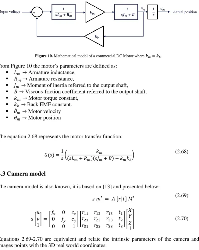
The flexion and rotation of JAIMYTM are driven by two DC motors. A DC motor model is a well-known model (see [11] for instance). Hence the motor model is represented in Figure 10.

Figure 10. Mathematical model of a commercial DC Motor where 𝒌𝒎= 𝒌𝒃. From Figure 10 the motor’s parameters are defined as:

 𝐿_𝑚 → Armature inductance,

 𝑅_𝑚 → Armature resistance,

 𝐽𝑚 → Moment of inertia referred to the output shaft,

 𝐵 → Viscous-friction coefficient referred to the output shaft,

 𝑘𝑚 → Motor torque constant,

 𝑘𝑏→ Back EMF constant.

 𝜃̇𝑚 → Motor velocity

 𝜃𝑚 → Motor position

The equation 2.68 represents the motor transfer function:

𝐺(𝑠) =1

The camera model is also known, it is based on [13] and presented below:

15

 (𝑋, 𝑌, 𝑍) → are the coordinates of a 3D point in the real world,

 (𝑢, 𝑣) → coordinates of projection point in pixels.

 𝐴 → camera matrix of intrinsic parameters,

 (𝑐𝑥, 𝑐𝑦) → principal point,

 𝑓𝑥, 𝑓𝑦 → focal lengths expressed in pixel units,

 𝑟 → rotation matrix,

 𝑡 → translation matrix,

 (𝑘₁, 𝑘₂, 𝑝₁, 𝑝₂, 𝑘₃) → Distortion coefficients are also needed.

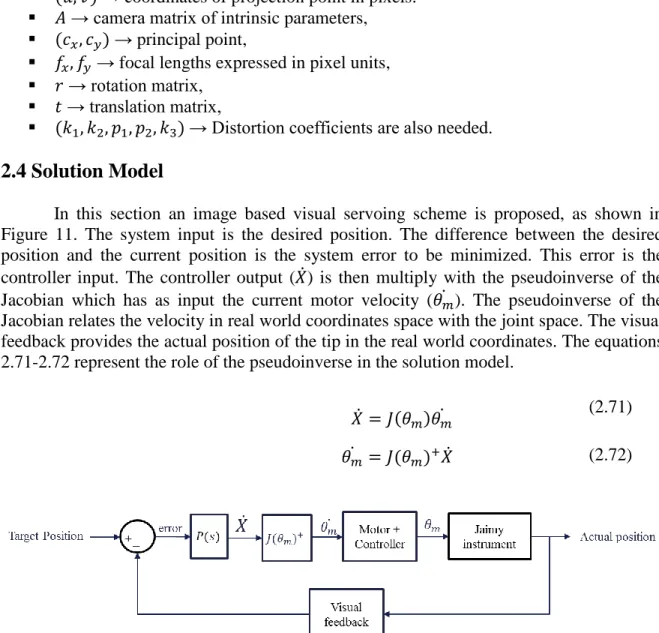
2.4 Solution Model

In this section an image based visual servoing scheme is proposed, as shown in Figure 11. The system input is the desired position. The difference between the desired position and the current position is the system error to be minimized. This error is the controller input. The controller output (𝑋̇) is then multiply with the pseudoinverse of the Jacobian which has as input the current motor velocity (𝜃_𝑚̇ ). The pseudoinverse of the Jacobian relates the velocity in real world coordinates space with the joint space. The visual feedback provides the actual position of the tip in the real world coordinates. The equations 2.71-2.72 represent the role of the pseudoinverse in the solution model.

𝑋̇ = 𝐽(𝜃𝑚)𝜃𝑚̇ (2.71)

𝜃_𝑚̇ = 𝐽(𝜃_𝑚)+_{𝑋̇ (2.72)}

16

Chapter 3

Simulation

This chapter describes simulations done using Matlab in order to validate the kinematic model, for this purpose an ideal motor model is used.

3.1 Simulation of kinematic model with ideal plant

In section 2.1 the kinematic model of the JAIMYTM instrument was determined. The equations 2.48-2.49 represent the position of the end-effector with respect to JAIMYTM base frame. In order to validate the kinematic model a closed loop configuration is implemented. The dc motor model is considered ideal. Figure 12 shows the structure of the closed loop. The simulation consisted in entering a desired angle of flexion in the left input block, the second block (Desired position) compute the components (𝑥_𝑑, 𝑦_𝑑) of the desired position from a given angle. The Kinematic model block determines the components

(𝑥_𝑎, 𝑦_𝑎) of the actual position. A simple proportional gain is considered. The pseudoinverse of the Jacobian receives the controller output and the current angular position to finally feed the last block to implement the system animation. An oscilloscope has been added to visualize the input position angle versus the actual angle.

Figure 12. Closed loop to validate the kinematic model.

To verify if the simulation is correct the relation expressed in equation 2.18 is used. This equation represents half the angle of end-effector with respect to the axis 𝑦 of instrument base frame; it is illustrated in Figure 9, so that equation can be expressed as follow:

𝜃_𝐼 = 2𝜃 =𝑟𝑝𝜃𝑚 𝑟

(3.1)

where 𝜃_𝐼 is the angle of instrument tip.

Equation 3.1 is used to compute the expected angle of the tip after simulation. The result is presented in Figure 13, for this simulation the desired position angle entered is 𝜃_𝑚 =

17

18

Chapter 4

Experimental Evaluation

The experimental evaluation of proposed control scheme is described in this chapter. First, a platform overview is described. Second, camera calibration stereo is detailed. Then, the software developed is introduced. Finally, system identification and experimental results are presented.

4.1 Platform Description

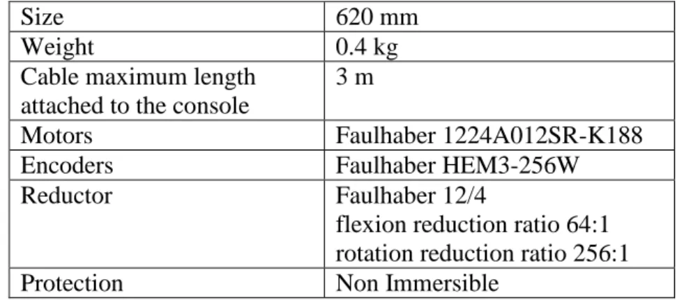
As already mentioned before, Figure 1 shows a general description of the proposed solution. It has four general components. The first one is the hand-held surgical instrument. Table 1 summarizes the technical characteristics of the JAIMYTM.

Size 620 mm

Table 1. Technical characteristics of the JAIMYTM.

The Controller Device is the input to the surgical instrument, which is in charge of controlling the flexion-rotation motions of JAIMYTM motors. The hardware used to control the motors is EPOS3 from maxon motor. It will be described in section 4.1.1. Refer to [14] for further details. The Image processing PC/Visualization incorporates the User Interface (section 4.1.4) which implements the algorithms to process the images taken from the Stereo Camera (section 4.1.2), the communication software, motion commands and visualization.

4.1.1 Controller Device

19

Figure 14. Controller architecture implemented by the EPOS3.

To determine the appropriate values for the parameters of each PI controller the auto tuning function of EPOS Studio software is used. This software is provided by maxon motor. Since the motors of JAIMYTM have load attached, the auto tuning give an appropriate response for the current controller but is not enough in the case of velocity controller. As a consequence, a manual tuning is required to get a better response for this case, Figure 15 shows the response for the current controller after auto tuning. It can be observed that the current actual value in red is following to the current demand value in blue and it is under the maximal admissible current 440mA as expected, see [15].

Figure 15. Current controller response after auto tuning, blue → current demand value, red → current actual value.

Figure 16 shows the velocity controller response after manual tuning, from this data the velocity demand value is 3000 rpm, the arithmetic average of the velocity actual value is 3000.84 rpm with a standard deviation of 10.48 rpm between 0.20 and 1 second in steady state, for the purpose of this project this response is acceptable.

-100.00 -50.00 0.00 50.00 100.00 150.00 200.00 250.00

0.00 0.10 0.20 0.30 0.40 0.50 0.60 0.70 0.80 0.90 1.00

Current (mA)

20

Figure 16. Velocity controller response after manual tuning, blue → velocity demand value, red → velocity actual value.

4.1.2 Camera Stereo Calibration

The camera stereo calibration is done based on the algorithms described in the chapter 12 of [16]. 25 pair images of a chessboard of 54 internal corners with a square size of 7.5mm are used. Figure 17 shows one of the image pairs used to do the stereo calibration. The cameras used are two scA640-70fc by Basler AG [17] plus two endoscopic lenses attached to them. These lenses are from Karl Storz. Figure 18 displays the whole setup of endoscope, cameras and JAIMYTM.

Figure 17. First pair image of the pictures used to do the stereo calibration.

0.00 500.00 1000.00 1500.00 2000.00 2500.00 3000.00 3500.00

0.00 0.10 0.20 0.30 0.40 0.50 0.60 0.70 0.80 0.90 1.00

Velocity (rpm)

21

Figure 18. Endoscopic lenses plus Basler cameras setup.

4.1.3 System Identification

Equations 2.48-2.49 represent the position of the tip with respect to JAIMYTM base frame. From those equations, 𝑟, 𝐿 and 𝐼 are known. As mentioned before in section 3.1 the pulley (𝑟𝑝) radius is missing therefore an identification procedure is needed. In order to

identify the missing parameter, the equation 3.1 is used. After the stereo camera system is calibrated and the tracking algorithms are implemented, experimental values 𝜃_𝐼 are taken by using the stereo vision feedback, these values are presented in Table 2. Figure 19 shows the tip of JAIMYTM being tracked by using green markers. The points 𝑃₁, 𝑃₂, 𝑃₃ and 𝑃₄ are located strategically in order to make easier tracking the object, the vector 𝐴⃗ = 𝑃⃗⃗⃗⃗⃗⃗⃗⃗⃗₁𝑃₂ is used to define JAIMYTM base frame, whereas 𝐵⃗⃗ = 𝑃⃗⃗⃗⃗⃗⃗⃗⃗⃗3𝑃4 represent the instrument rigid section.

The point 𝑃2 is considered as the origin of JAIMYTM base frame and the beginning of

flexible section, and 𝑃₃ the end of this section. Since the stereo camera system is already calibrated, it is possible to get the real 3D information of those points. Accordingly the real angle between the vectors 𝐴⃗ and 𝐵⃗⃗ can be measured, this angle is 𝜃_𝐼.

Figure 19. Image of the tip of the JAIMYTM being tracked by using markers.

𝑷_𝟏 𝑷_𝟐 𝑷_𝟑

𝑷_𝟒 𝑨

⃗⃗⃗

22 It can be observed from equation 3.1 that the angle of instrument tip (𝜃_𝐼) is linearly related with the motor angle (𝜃𝑚), being 𝜃𝐼 the product of 𝜃𝑚 multiplied by the constant factor𝑟_𝑟𝑝.

Therefore this expression is in the form of a linear equation as shown below:

𝑦 = 𝑚𝑥 + 𝑏 (4.1) equation 4.3 with the experimental data collected in Table 2.

Table 2 presents the collected data for the optimization procedure in order to estimate the pulley radius. The variable 𝜃_𝑚𝑗 is the experimental value of motor angle, 𝜃_𝐼𝑗 is the tip angle experimental value and 𝑒 is the squared error function to be minimized. The value of 𝜃_𝐼𝑗and

23

0.078 𝑚𝑚 and 𝑒 = 0.0149 (𝑟𝑎𝑑)2. The method of linear regression is also used in order to verify the previously estimated value. For this case the Matlab Curve Fitting Tool is used.

Figure 20. Linear regression method to estimate the radius of the pulley.

Figure 20 shows the result of optimization using the linear regression method. The resulting slope after optimization is 𝑚 = 0.0313, it was mentioned before that this data represents the factor 𝑟_𝑟𝑝, and knowing that 𝑟 = 2.5 𝑚𝑚 then 𝑟𝑝 = 0,078 𝑚𝑚. It is important to

mention that the parameters 𝑚 and 𝑏 in the Matlab Curve Fitting Tool were limited to be equal or greater than 0, since they cannot be negative for the real system. The adjusted

𝑅𝑠𝑞𝑢𝑎𝑟𝑒 and 𝑅𝑠𝑞𝑢𝑎𝑟𝑒 are equal to 0.9947, it means that the estimated model explains the

99,47% of the variation in the experimental data, the values for SSE (sum of squares due to error) and RMSE (Root Mean Squared Error) are 0.0149 𝑟𝑎𝑑2 and 0.03268 𝑟𝑎𝑑 correspondingly. RMSE represents the standard deviation. For the estimated value of 𝑟𝑝, the

same value was obtained and verified from both optimization tools. Therefore is possible to predict values of 𝜃_𝐼 based on 𝜃_𝑚 with 99,47% of goodness with a standard deviation of

0.03268 𝑟𝑎𝑑.

4.1.4 Software

Image processing, visualization and user interaction are done by software running in a PC workstation HP Z400. This software implements all the algorithms to process the images to track the JAIMYTM tip and determining its 3D location with respect to the point of interest. It also performs the EtherCAT communication with the EPOS3, and provides the user interface to control the motion of JAIMYTM motors. The software is developed using QT libraries [18] for the user interface, OpenCV [19] for image processing and Debian 8 [20] as operating system and the EhterCAT drivers for linux provided by [21] to communicate with EPOS3. The Figure 21 below describes the user interface developed to control the system.

0.00 10.00 20.00 30.00 40.00 50.00

24

Figure 21. User interface developed to control the system.

Figure 22 shows the block diagram of the solution including the hardware and software. The software flow diagram starts after receiving the image information from the cameras via Firewire. The user makes the segmentation of the green markers manually; the user interface provides this functionality. After the segmentation is done, the BGR image is converted to HSV representation, then the hue histogram of each marker is extracted and filtered by back projection [22]. The Camshift algorithm [23] is used to track the markers using the histogram and the back projection image. Since the stereo calibration is already done, the intrinsic and extrinsic parameters of the camera are known, therefore the relation between the image plane and the real world coordinates is also known. Using the parameters of the camera and the block matching algorithm [24] to find stereo correspondences the disparity map is computed. From the disparity map and the relation 4.4 (also refer to [13]) the 3D map information is also calculated. Once having those information maps that relates the image pixels and the 3D real world coordinates, the location of each pixel of the image with disparity is known with respect to the camera base frame, it includes the location of the markers and any other point which disparity information has been found. It is important to mention that the algorithms used to find stereo correspondences and 3D reconstruction are implemented by using OpenCV libraries, in this case the CUDA support is used to make the image processing faster. Mathematical computations block in Figure 22 uses the disparity/3D map information, the location of the markers and the point of interest to determine the real position of the point of interest with respect to JAIMYTM base frame. Besides to implementing the pseudoinverse of the Jacobian to compute the velocity demand value (𝜃_𝑚̇ ), this demand velocity value is sent by the EPOS3 commands library trough the linux based EtherCAT drivers, it is important to mention that the software is also reading the position actual value (𝜃𝑚) from the EPOS3 via

EtherCAT communication.

25

Figure 22. Block diagram of the solution.

Another important task done by the Mathematical computations block is calculating the relation between the JAIMYTM base frame and the camera’s frame, this is done by defining the vectors 𝑷⃗⃗⃗⃗⃗⃗_𝟐, 𝑨⃗⃗⃗ and 𝑩⃗⃗⃗ from Figure 19 as:

𝑷_𝟐

⃗⃗⃗⃗⃗⃗= 𝑷_𝟐𝒙+ 𝑷_𝟐𝒚+ 𝑷_𝟐𝒛 (4.5)

𝑨

⃗⃗⃗ = 𝑷⃗⃗⃗⃗⃗⃗⃗⃗⃗⃗⃗𝟏𝑷𝟐 (4.6)

𝑩

⃗⃗⃗ = 𝑷⃗⃗⃗⃗⃗⃗⃗⃗⃗⃗⃗𝟑𝑷𝟒 (4.7)

Considering unit vector of 𝑨⃗⃗⃗ as the axis 𝑥 of JAIMYTM base frame:

𝒙𝒖

⃗⃗⃗⃗⃗ = 𝑨⃗⃗⃗

‖𝑨⃗⃗⃗‖= 𝒙𝒖𝒙𝒙̂ + 𝒙𝒖𝒚𝒚̂ + 𝒙𝒖𝒛𝒛̂ (4.8)

Unit vector of axis 𝑧 of JAIMYTM base frame:

𝒛_𝒖

⃗⃗⃗⃗⃗ = 𝑨⃗⃗⃗ × 𝑩⃗⃗⃗

‖𝑨⃗⃗⃗ × 𝑩⃗⃗⃗‖= 𝒛𝒖𝒙𝒙̂ + 𝒛𝒖𝒚𝒚̂ + 𝒛𝒖𝒛𝒛̂ (4.9)

26 JAIMYTM base frame origin with respect to the camera base frame.

4.2 Experimental Results

This section describes the experimental results obtained after implementing the solution proposed in page 1. The kinematic model was determined in chapter 1 in order to implement the Jacobian which is the element that relates the real world coordinates space with the joint space. The missing parameter, pulley radius 𝑟_𝑝 was experimentally identified in section 4.2. The velocity controller device used and its PI controller explained in section 4.1.1, the camera stereo calibration and the user interface were also presented in chapter 4. This section presents functional results after putting together the solution´s components previously mentioned.

The system functionality consists in choosing a point in the workspace of the instrument by using the visual feedback, then the system will pose the tip of the JAIMYTM in the desired position, Figure 23 shows the experiments when the system is positioning the tip of the instrument in the desired point, from the picture the error for the component 𝑥 is

−0.857 𝑚𝑚 and the error for component 𝑦 is 0.0889 𝑚𝑚, error less than 1 mm in both axis, all the values are in mm, the final velocity is 0 rpm, which means that the system has reached the steady state.

27

Figure 23. Automatic positioning of the tip of the JAIMYTM in the desired point.

Figure 24 shows the position response of the system for a given desired point, for this experiment the desired point is (𝑥_𝑑, 𝑦_𝑑) = (39.50, 34.14), the final position reached in steady state is (𝑥_𝑎, 𝑦_𝑎) = (39.27, 34.50), the error for the component 𝑥 is 0.23 𝑚𝑚 and the error for the component 𝑦 is −0.36 𝑚𝑚, error less than 1 mm in both axis. It is important to mention that this response is being affected by the noise caused for the variation of the image amount frames, improving the image processing and tracking algorithm this noise can be reduced.

Figure 24. Position response of the system.

Figure 25 displays the velocity response for the same experiment in Figure 23, this graphic shows in blue the velocity demand value and the actual value in red. The velocity actual value is following the velocity demand value as expected. The velocity is increased in order to reach the desired position and then decreased as the error is being reduced.

39.50

0.00 1.00 2.00 3.00 4.00 5.00

28

Figure 25. Velocity response of the system.

Figure 26 presents the disparity map and 3D information for different block sizes of the same image. This information is used by the software that implements the tracking and visual control algorithms. The disparity map represents the differences between the stereoscopic images, then by reprojecting the disparity map to 3D space the 3D map information is obtained, images b) and d) are the disparity maps, images c) and e) the corresponding 3D map information. It can be observed that the smaller is the block size the more difficult is to find the disparities and more details can be observed, therefore the higher is the block size the easier is to find the disparities and less details can be observed. Hence a trade-off between the detail of the image and the smoothness of the disparity must be stablished. For this project, it is experimentally determined that a block size between 17 and 29 works properly.

0.00 1.00 2.00 3.00 4.00 5.00 6.00

29

a) b)

c) d)

e)

30

Conclusions and Perspectives

In this thesis, the development of a system with the capability of assisting surgeons to pose the end-effector of the JAIMYTM instrument is presented as the main objective; it is done by using stereoscopic vision feedback. As part of the work flow to reach the general objective, specific objectives in Introduction section are proposed, concluding the following:

 For the specific objective of determining the kinematic model of the instrument, it is determined and validated in a closed loop simulation; refer to sections 3.1-3.2.

 Missing parameter radius of the pulley identification is successfully estimated.

 For the objective of using stereoscopic vision as feedback to estimate the actual position of the instrument and the point of interest, it is developed according to Figure 11, with a unit proportional gain.

 The position controller of the system provides a response with an error less than 1 mm in steady state based on the data presented in Figure 23 and Figure 24.

The general and specific objectives have been reached during the project development, the probe of concept of its functionality has been successfully validated, however there is more work to do in order to improve the system and make it feasible in real surgical environment, it is translated as next steps for futures works, such as the implementation of a profile to reach the desired position to help avoiding high velocity steps at the moment of positioning the tip of the instrument, besides of improving the controller position response by adjusting the controller parameters instead of using only a unit proportional gain, also knowing the camera parameters is possible to add augmented reality to provide more information to be displayed to improve assistance during the surgical procedure. Another important improvement would be taking advantage of the new JAIMYTM’s version with bidirectional flexion motion, also improving the algorithms to track the instrument and 3D reconstruction can reduce the noise affecting the position controller, a measurement of the accuracy of the system is also needed with the appropriate instrumentation since the scope of this stage of the project was focus on functional results not in accuracy.

31

Bibliography

[1] LIRMM, “DEXTER / Teams / Research / Homepage / Lirmm.fr / - LIRMM,”

www.lirmm.fr, 2014. [Online]. Available:

http://www.lirmm.fr/lirmm_eng/research/teams/dexter. [Accessed: 23-Nov-2015]. [2] Endocontrol, “JAIMYTM - Endocontrol,” 2015. [Online]. Available:

http://www.endocontrol-medical.com/produits/jaimy-oui/. [Accessed: 24-Nov-2015]. [3] F. Tendick, S. S. Sastry, R. S. Fearing, and M. Cohn, “Applications of

micromechatronics in minimally invasive surgery,” IEEE/ASME Trans. Mechatronics, vol. 3, no. 1, pp. 34–42, Mar. 1998.

[4] A. Krupa, J. Gangloff, C. Doignon, M. F. de Mathelin, G. Morel, J. Leroy, L. Soler, and J. Marescaux, “Autonomous 3-d positioning of surgical instruments in robotized laparoscopic surgery using visual servoing,” IEEE Trans. Robot. Autom., vol. 19, no. 5, pp. 842–853, Oct. 2003.

[5] P. Hynes, G. I. Dodds, and A. J. Wilkinson, “Uncalibrated Visual-Servoing of a Dual-Arm Robot for MIS Suturing,” in The First IEEE/RAS-EMBS International Conference on Biomedical Robotics and Biomechatronics, 2006. BioRob 2006., 2006, pp. 420–425.

[6] B. C. Becker, C. R. Valdivieso, J. Biswas, L. A. Lobes, and C. N. Riviere, “Active guidance for laser retinal surgery with a handheld instrument.,” Conf. Proc. ... Annu. Int. Conf. IEEE Eng. Med. Biol. Soc. IEEE Eng. Med. Biol. Soc. Annu. Conf., vol. 2009, pp. 5587–90, Jan. 2009.

[7] B. C. Becker, R. A. Maclachlan, L. A. Lobes, G. D. Hager, and C. N. Riviere, “Vision-Based Control of a Handheld Surgical Micromanipulator with Virtual Fixtures.,” IEEE Trans. Robot., vol. 29, no. 3, pp. 674–683, Feb. 2013.

[8] A. Agustinos, R. Wolf, J. A. Long, P. Cinquin, and S. Voros, “Visual servoing of a robotic endoscope holder based on surgical instrument tracking,” in 5th IEEE RAS/EMBS International Conference on Biomedical Robotics and Biomechatronics, 2014, pp. 13–18.

[9] R. Reilink, S. Stramigioli, and S. Misra, “3D position estimation of flexible

instruments: marker-less and marker-based methods.,” Int. J. Comput. Assist. Radiol. Surg., vol. 8, no. 3, pp. 407–17, May 2013.

[10] P. Cabras, D. Goyard, F. Nageotte, P. Zanne, and C. Doignon, “Comparison of methods for estimating the position of actuated instruments in flexible endoscopic surgery,” in 2014 IEEE/RSJ International Conference on Intelligent Robots and Systems, 2014, pp. 3522–3528.

[11] Katsuhiko Ogata, Modern Control Engineering, 5/E, 5th ed. Pearson, 2010. [12] F. Monasterio-Huelin and Á. Gutiérrez, “Modelo lineal de un motor de corriente

continua.,” Robolabo, 2012. [Online]. Available:

http://www.robolabo.etsit.upm.es/asignaturas/seco/apuntes/motor_dc.pdf. [Accessed: 01-Dec-2015].

[13] OpenCV, “Camera Calibration and 3D Reconstruction — OpenCV 2.4.12.0 documentation.” [Online]. Available:

32 [14] “maxon motor - Online Shop.” [Online]. Available:

http://www.maxonmotor.com/maxon/view/product/control/Positionierung/411146?et cc_med=1column&etcc_cmp=comp_00003AC8&etcc_cu=onsite&etcc_var=%5bco m%5d%23en%23_d_&etcc_plc=product_overview_controller_epos. [Accessed: 04-Dec-2015].

[15] “FAULHABER.” [Online]. Available:

https://fmcc.faulhaber.com/details/overview/PGR_1049_13818/PGR_13818_13813/ en/GLOBAL/#. [Accessed: 04-Dec-2015].

[16] G. Bradski and A. Kaehler, Learning OpenCV - O’Reilly Media, First Edit. O’Reilly

Media, 2008.

[17] “Basler scout scA640-70fc - Area Scan Camera.” [Online]. Available:

http://www.baslerweb.com/en/products/area-scan-cameras/scout/sca640-70fc. [Accessed: 07-Dec-2015].

[18] “Qt.” [Online]. Available: https://www.qt.io/. [Accessed: 07-Dec-2015].

[19] “OpenCV | OpenCV.” [Online]. Available: http://opencv.org/. [Accessed: 07-Dec-2015].

[20] “Debian -- El sistema operativo universal.” [Online]. Available: https://www.debian.org/. [Accessed: 07-Dec-2015].

[21] “IgH EtherCAT Master for Linux.” [Online]. Available:

http://www.etherlab.org/en/ethercat/index.php. [Accessed: 07-Dec-2015]. [22] “Back Projection — OpenCV 2.4.12.0 documentation.” [Online]. Available:

http://docs.opencv.org/2.4/doc/tutorials/imgproc/histograms/back_projection/back_p rojection.html. [Accessed: 09-Dec-2015].

[23] “OpenCV: Meanshift and Camshift.” [Online]. Available:

http://docs.opencv.org/master/db/df8/tutorial_py_meanshift.html#gsc.tab=0. [Accessed: 09-Dec-2015].

[24] “OpenCV: cv::cuda::StereoBM Class Reference.” [Online]. Available:

http://docs.opencv.org/master/db/d8a/classcv_1_1cuda_1_1StereoBM.html#gsc.tab= 0. [Accessed: 09-Dec-2015].

[25] Maxon motor, “EPOS3 ETherCAT Position Controllers, Firmware Specification,” 2014. [Online]. Available:

http://www.maxonmotor.com/medias/sys_master/root/8815100592158/EPOS3-EtherCAT-Firmware-Specification-En.pdf. [Accessed: 11-Dec-2015].

[26] “IgH EtherCAT Master 1.52 Documentation.” [Online]. Available:

http://www.etherlab.org/download/ethercat/ethercat-1.5.2.pdf. [Accessed: 17-Dec-2015].

[27] “Quadro 4000 – Workstation graphics card for 3D design, styling, visualization, CAD, and more.” [Online]. Available: http://www.nvidia.com/object/product-quadro-4000-us.html. [Accessed: 16-Dec-2015].

[28] Endocontrol, JAiMY - SPY Manuel Utilisateur. EndoControl, 2013. [29] Maxon motor, “EPOS3 70/10 EtherCAT Positioning Controller Hardware

Reference,” 2014. [Online]. Available:

33

Appendix A

A.1 PI Controller Parameters, units conversion EPOS3 to SI Units

𝐾𝑃_𝑆𝐼 = 20

𝜇𝐴

(𝑟𝑎𝑑/𝑠)∙ 𝐾𝑃_𝐸𝑃𝑂𝑆3 A.1.1

𝐾_{𝐼_𝑆𝐼} = 5 𝑚𝐴/𝑠

(𝑟𝑎𝑑/𝑠)∙ 𝐾𝐼_𝐸𝑃𝑂𝑆3 A.1.2

A.2 EPOS3 state machine

34

Command LowByte of Controlword [binary]

*1) Automatic transition to “Enable Operation” after executing “Switched On” functionality.

Table 3. Device control commands, taken from [25].

A.3 Software components

 Debian

Operating system https://www.debian.org/

 Camwire

Generic Firewire camera communication in linux http://kauri.auck.irl.cri.nz/~johanns/camwire/

 Ethercat version: 1.52

Linux driver

http://www.etherlab.org/en/ethercat/index.php

Suggestion of configuration for Ethercat driver installation:

./configure --with-linux-dir=/usr/src/linux --enable-8139too=no --enable-cycles=yes --with-e1000e-kernel=yes

Check if the NIC is compatible with the Ethercat driver, look for the linux kernel that support your hardware:

http://www.etherlab.org/en/ethercat/hardware.php Refer to [26] for further details about installation.

 QT Libraries

 Download and install QTCreator.

https://www.qt.io/download-open-source/

 Install opengl libraries for qt

$sudo apt-get install libqt5opengl5-dev

 OpenCV

http://opencv.org/

 CUDA Toolkit

35 A.4 Graphic card information

GPU Specs:

NVIDIA Quadro GPU Quadro 4000

CUDA Cores 256

Total Frame Buffer 2 GB GDDR5

Memory Interface 256-bit

Memory Bandwidth

(GB/sec) 89.6 GB/s Software

Linux NVIDIA Driver

versión 340.52 Cuda Toolkit version 6.5

Table 4. Graphic card specifications used in the project, refer to [27].

A.5 Connections

JAIMYTM,Sub-d connector 15 wires 1: + flexion motor 2: - flexion motor 10: channel 𝑍 rotation encoder 11: GND flexion encoder 12: GND rotation encoder 13: +2.5V

14: setpoint rotation 15: setpoint flexion

EPOS3 Encoder connector J4 1: do not connect 2: +5 VDC / 100mA

EPOS3 Power supply connector 1 Ground of supply voltage 2 +VCC, Power supply voltage