Identification and energy calibration of hadronically decaying tau leptons with the ATLAS experiment in pp collisions at root s=8 TeV

Texto completo

(1)EUROPEAN ORGANISATION FOR NUCLEAR RESEARCH (CERN). CERN-PH-EP-2014-227. arXiv:1412.7086v2 [hep-ex] 15 Jul 2015. Submitted to: Eur. Phys. J. C. Identification and energy calibration of hadronically decaying tau leptons with the ATLAS √ experiment in pp collisions at s=8 TeV. The ATLAS Collaboration. Abstract This paper describes the trigger and offline reconstruction, identification and energy calibration algorithms for hadronic decays of tau leptons employed for the data collected from pp collisions in √ 2012 with the ATLAS detector at the LHC center-of-mass energy s = 8 TeV. The performance of these algorithms is measured in most cases with Z decays to tau leptons using the full 2012 dataset, corresponding to an integrated luminosity of 20.3 fb−1 . An uncertainty on the offline reconstructed tau energy scale of 2 − 4%, depending on transverse energy and pseudorapidity, is achieved using two independent methods. The offline tau identification efficiency is measured with a precision of 2.5% for hadronically decaying tau leptons with one associated track, and of 4% for the case of three associated tracks, inclusive in pseudorapidity and for a visible transverse energy greater than 20 GeV. For hadronic tau lepton decays selected by offline algorithms, the tau trigger identification efficiency is measured with a precision of 2 − 8%, depending on the transverse energy. The performance of the tau algorithms, both offline and at the trigger level, is found to be stable with respect to the number of concurrent proton-proton interactions and has supported a variety of physics results using hadronically decaying tau leptons at ATLAS.. c 2015 CERN for the benefit of the ATLAS Collaboration. Reproduction of this article or parts of it is allowed as specified in the CC-BY-3.0 license..

(2) Noname manuscript No. (will be inserted by the editor). Identification and energy calibration of hadronically decaying tau √ leptons with the ATLAS experiment in pp collisions at s=8 TeV The ATLAS Collaboration. Received: date / Accepted: date. Abstract This paper describes the trigger and offline reconstruction, identification and energy calibration algorithms for hadronic decays of tau leptons employed for the data collected from pp collisions in 2012 with the ATLAS detector at the LHC center-of-mass energy √ s = 8 TeV. The performance of these algorithms is measured in most cases with Z decays to tau leptons using the full 2012 dataset, corresponding to an integrated luminosity of 20.3 fb−1 . An uncertainty on the offline reconstructed tau energy scale of 2−4%, depending on transverse energy and pseudorapidity, is achieved using two independent methods. The offline tau identification efficiency is measured with a precision of 2.5% for hadronically decaying tau leptons with one associated track, and of 4% for the case of three associated tracks, inclusive in pseudorapidity and for a visible transverse energy greater than 20 GeV. For hadronic tau lepton decays selected by offline algorithms, the tau trigger identification efficiency is measured with a precision of 2 − 8%, depending on the transverse energy. The performance of the tau algorithms, both offline and at the trigger level, is found to be stable with respect to the number of concurrent proton-proton interactions and has supported a variety of physics results using hadronically decaying tau leptons at ATLAS. Keywords LHC · ATLAS · tau 1 Introduction With a mass of 1.777 GeV and a proper decay length of 87 µm [1], tau leptons decay either leptonically (τ → ℓνℓ ντ , ℓ = e, µ) or hadronically (τ → hadrons ντ , denoted τhad ) and do so typically before reaching active. regions of the ATLAS detector. They can thus only be identified via their decay products. In this paper, only hadronic tau lepton decays are considered. The hadronic tau lepton decays represent 65% of all possible decay modes [1]. In these, the hadronic decay products are one or three charged pions in 72% and 22% of all cases, respectively. Charged kaons are present in the majority of the remaining hadronic decays. In 78% of all hadronic decays, up to one associated neutral pion is also produced. The neutral and charged hadrons stemming from the tau lepton decay make up the visible decay products of the tau lepton, and are in the following referred to as τhad-vis . The main background to hadronic tau lepton decays is from jets of energetic hadrons produced via the fragmentation of quarks and gluons. This background is already present at trigger level (also referred to as online in the following). Other important backgrounds are electrons and, to a lesser degree, muons, which can mimic the signature of tau lepton decays with one charged hadron. In the context of both the trigger and the offline event reconstruction (shortened to simply offline in the following), discriminating variables based on the narrow shower shape, the distinct number of charged particle tracks and the displaced tau lepton decay vertex are used. Final states with hadronically decaying tau leptons are an important part of the ATLAS physics program. Examples are measurements of Standard Model processes [2,3,4,5,6], Higgs boson searches [7], searches for new physics such as Higgs bosons in models with extended Higgs sectors [8,9,10], supersymmetry (SUSY) [12,13,11], heavy gauge bosons [14] and leptoquarks [15]. This places strong requirements on the τhad-vis identification algorithms (in the following, referred to as tau identification): robustness and high.

(3) 2. performance over at least two orders of magnitude in transverse momentum with respect to the beam axis (pT ) of τhad-vis , from about 15 GeV (decays of W and Z bosons or scalar tau leptons) to a few hundred GeV (SUSY Higgs boson searches) and up to beyond 1 TeV (Z ′ searches). At the same time, an excellent energy resolution and small energy scale uncertainty are particularly important where resonances decaying to tau leptons need to be separated (e.g. Z → τ τ from H → τ τ mass peaks). The triggering for final states which rely exclusively on tau triggers is particularly challenging, e.g. H → τ τ where both tau leptons decay hadronically. At the trigger level, in addition to the challenges of offline tau identification, bandwidth and time constraints need to be satisfied and the trigger identification is based on an incomplete reconstruction of the event. The ATLAS trigger system, together with the detector and the simulation samples used for the studies presented, are briefly described in Sect. 2. The ATLAS offline tau identification uses various discriminating variables combined in Boosted Decision Trees (BDT) [16,17] to reject jets and electrons. The offline tau energy scale is set by first applying a local hadronic calibration (LC) [18] appropriate for a wide range of objects and then an additional tau-specific correction based on simulation. The online tau identification is implemented in three different steps, as is required by the ATLAS trigger system architecture [19]. The same identification and energy calibration procedures as for offline are used in the third level of the trigger, while the first and second trigger levels rely on coarser identification and energy calibration procedures. A description of the trigger and offline τhad-vis reconstruction and identification algorithms is presented in Sect. 3, and the trigger and offline energy calibration algorithms are discussed in Sect. 5. The efficiency of the identification and the energy scale are measured in dedicated studies using a Z → τ τ enhanced event sample of collision data recorded by the ATLAS detector [20] at the LHC [21] in 2012 at a centre-of-mass energy of 8 TeV. This is described in Sect. 4 and Sect. 5. Conclusions and outlook are presented in Sect. 6. 2 ATLAS detector and simulation 2.1 The ATLAS detector The ATLAS detector [20] consists of an inner tracking system surrounded by a superconducting solenoid, electromagnetic (EM) and hadronic (HAD) calorimeters, and a muon spectrometer (MS). The inner detector (ID) is immersed in a 2 T axial magnetic field, and. The ATLAS Collaboration. consists of pixel and silicon microstrip (SCT) detectors inside a transition radiation tracker (TRT), providing charged-particle tracking in the region |η| < 2.5.1 The EM calorimeter uses lead and liquid argon (LAr) as absorber and active material, respectively. In the central rapidity region, the EM calorimeter is divided in three layers, one of them segmented in thin η strips for optimal γ/π 0 separation, and completed by a presampler layer for |η| < 1.8. Hadron calorimetry is based on different detector technologies, with scintillator tiles (|η| < 1.7) or LAr (1.5 < |η| < 4.9) as active medium, and with steel, copper, or tungsten as the absorber material. The calorimeters provide coverage within |η| < 4.9. The MS consists of superconducting air-core toroids, a system of trigger chambers covering the range |η| < 2.4, and high-precision tracking chambers allowing muon momentum measurements within |η| < 2.7. Physics objects are identified using their specific detector signatures; electrons are reconstructed by matching a track from the ID to an energy deposit in the calorimeters [22,23], while muons are reconstructed using tracks from the MS and ID [24]. Jets are reconstructed using the anti-kt algorithm [25] with a distance parameter R = 0.4. Three-dimensional clusters of calorimeter cells called TopoClusters [26], calibrated using a local hadronic calibration [18], serve as inputs to the jet algorithm. The missing transverse momentum miss (with magnitude ET ) is computed from the combination of all reconstructed physics objects and the remaining calorimeter energy deposits not included in these objects [27]. The ATLAS trigger system [19] consists of three levels; the first level (L1) is hardware-based while the second (L2) and third (Event Filter, EF) levels are software-based. The combination of L2 and the EF are referred to as the high-level trigger (HLT). The L1 trigger identifies regions-of-interest (RoI) using information from the calorimeters and the muon spectrometer. The delay between a beam crossing and the trigger decision (latency) is approximately 2 µs at L1. The L2 system typically takes the RoIs produced by L1 as input and refines the quantities used for selection after taking into account the information from all subsystems. The latency at L2 is on average 40 ms, but can be as large 1 ATLAS uses a right-handed coordinate system with its origin at the nominal interaction point (IP) in the centre of the detector and the z-axis along the beam direction. The xaxis points from the IP to the centre of the LHC ring, and the y-axis points upward. Cylindrical coordinates (r, φ) are used in the transverse (x, y) plane, φ being the azimuthal angle around the beam direction. The pseudorapidity is defined in terms of the polar angle θ as η = − ln tan(θ/2). The distance p ∆R in the η–φ space is defined as ∆R = (∆η)2 + (∆φ)2 ..

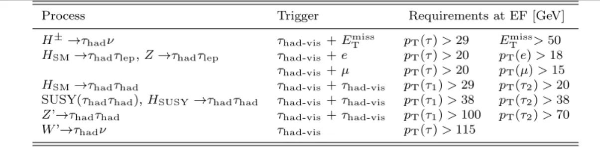
(4) Identification and energy calibration of hadronically decaying tau leptons in ATLAS at Process ±. H →τhad ν HSM →τhad τlep , Z →τhad τlep HSM →τhad τhad SUSY(τhad τhad ), HSUSY →τhad τhad Z’→τhad τhad W ’→τhad ν. Trigger τhad-vis τhad-vis τhad-vis τhad-vis τhad-vis τhad-vis τhad-vis. √. s=8 TeV. 3. Requirements at EF [GeV] + + + + + +. miss ET. e µ τhad-vis τhad-vis τhad-vis. pT (τ ) > 29 pT (τ ) > 20 pT (τ ) > 20 pT (τ1 ) > 29 pT (τ1 ) > 38 pT (τ1 ) > 100 pT (τ ) > 115. miss ET > 50 pT (e) > 18 pT (µ) > 15 pT (τ2 ) > 20 pT (τ2 ) > 38 pT (τ2 ) > 70. Table 1 Tau triggers with their corresponding kinematic requirements. Examples of physics processes targeted by each trigger are also listed, where τhad and τlep refer to hadronically and leptonically decaying tau leptons, respectively.. as 100 ms at the highest instantaneous luminosities. At the EF level, algorithms similar to those run in the offline reconstruction are used to select interesting events with an average latency of about 1 s. During 2012, the ATLAS detector was operated with a data-taking efficiency greater than 95%. The highest peak luminosity obtained was 8 · 1033 cm−2 s−1 at the end of 2012. The observed average number of pile-up interactions (meaning generally soft proton– proton interactions, superimposed on one hard proton– proton interaction) per bunch crossing in 2012 was 20.7. At the end of the data-taking period, the trigger system was routinely working with an average (peak) output rate of 700 Hz (1000 Hz).. 2.2 Tau trigger operation In 2012, a diverse set of tau triggers was implemented, using requirements on different final state configurations to maximize the sensitivity to a large range of physics processes. These triggers are listed in Table 1, along with the targeted physics processes and the associated kinematic requirements on the triggered objects. For the double hadronic triggers, in the lowest threshold version (29 and 20 GeV requirement on transverse momentum for the two τhad-vis ) two main criteria are applied: isolation at L12 , and full tau identification at the HLT. The isolation requirement is dropped for the intermediate threshold version, and both criteria are dropped in favour of a looser (more than 95% efficient), non-isolated trigger for the version with the highest thresholds. As the typical rejection rates of τhad-vis identification algorithms against the dominant multi-jet backgrounds are considerably smaller than those of electron or muon identification algorithms, τhad-vis triggers must have considerably higher pT requirements in order to maintain manageable trigger rates. Therefore, 2. A detailed definition of the isolation requirement is provided in Sect. 3.3.. most analyses using low-pT τhad-vis in 2012 depend on the use of triggers which identify other objects. However, by combining tau trigger requirements with requirements on other objects, lower thresholds can be accommodated for the tau trigger objects as well as the other objects. Figure 1 shows the tau trigger rates at L1 and the EF as a function of the instantaneous luminosity during the 8 TeV LHC operation. The trigger rates do not increase more than linearly with the luminosity, due the robust performance of the trigger algorithms under different pile-up conditions. The only exception is the miss τhad-vis + ET trigger, where the extra pile-up associated with the higher luminosity leads to a degradation miss of the resolution of the reconstructed event ET . At the highest instantaneous luminosities, the rates are affected by deadtime in the readout systems, leading to a general drop in the rates.. 2.3 Simulation and event samples The optimization and measurement of tau performance requires simulated events. Events with Z/γ ∗ and W boson production were generated using alpgen [28] interfaced to herwig [29] or Pythia6 [30] for fragmentation, hadronization and underlying-event (UE) modelling. In addition, Z → τ τ and W → τ ν events were generated using Pythia8 [31], and provide a larger statistical sample for the studies. For optimization at high pT , Z ′ → τ τ with Z ′ masses between 250 GeV and 1250 GeV were generated with Pythia8. Top-quark-pair as well as single-top-quark events were generated with mc@nlo+herwig [32], with the exception of t-channel single-top production, where AcerMC+Pythia6 [33] was used. W Z and ZZ diboson events were generated with herwig, and W W events with alpgen+herwig. In all samples with τ leptons, except for those simulated with Pythia8, Tauola [34] was used to model the τ decays, and Photos [35] was used for soft QED radiative corrections to particle decays..

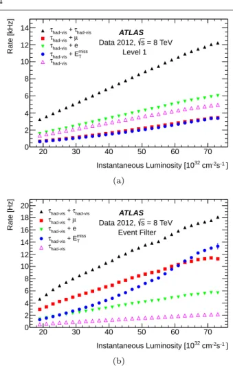
(5) The ATLAS Collaboration Rate [kHz]. 4 τhad-vis + τhad-vis τhad-vis + µ τhad-vis + e τhad-vis + Emiss T τhad-vis. 14 12 10. crossings (called pile-up). Prior to any analysis, the simulated events were reweighted such that the distribution of the number of pile-up interactions matched that in data. The simulated events were reconstructed with the same algorithm chain as used for collision data.. ATLAS Data 2012, s = 8 TeV Level 1. 8 6. 3 Reconstruction and identification of hadronic tau lepton decays. 4 2 0. 20. 30. 40. 50. 60. 70. Instantaneous Luminosity [1032 cm-2s-1 ]. Rate [Hz]. (a) 20. τhad-vis + τhad-vis τhad-vis + µ τhad-vis + e. 18 16. τhad-vis + Emiss T τhad-vis. 14. ATLAS Data 2012, s = 8 TeV Event Filter. 12 10 8. In the following, the τhad-vis reconstruction and identification at online and offline level are described. The trigger algorithms were optimized with respect to hadronic tau decays identified by the offline algorithms. This typically leads to online algorithms resembling their offline counterparts as closely as possible with the information available at a given trigger level. To reflect this, the details of the offline reconstruction and identification are described first, and then a discussion of the trigger algorithms follows, highlighting the differences between the two implementations.. 6 4. 3.1 Reconstruction. 2 0. 20. 30. 40. 50. 60. 70 32. Instantaneous Luminosity [10. cm-2s-1 ]. (b) Fig. 1 Tau trigger rates at (a) Level 1 and (b) √ Event Filter as a function of the instantaneous luminosity for s = 8 TeV. The triggers shown are described in Table 1, with the τhad-vis +τhad-vis being the rate for the lowest threshold trigger reported in the table. The rates for the higher threshold triggers are approximately three and five times lower at L1 and HLT, respectively, and are partially included in the rate of the lowest threshold item.. All events were produced using CTEQ6L1 [36] parton distribution functions (PDFs) except for the mc@nlo events, which used CT10 PDFs [37]. The UE simulation was tuned using collision data. Pythia8 events employed the AU2 tune [38], herwig events the AUET2 tune [39], while alpgen+Pythia6 used the Perugia2011C tune [40] and AcerMC+Pythia6 the AUET2B tune [41]. The response of the ATLAS detector was simulated using GEANT4 [42,43] with the hadronic-shower model QGSP BERT [44,45] as baseline. Alternative models (FTFP BERT [46] and QGSP) were used to estimate systematic uncertainties. Simulated events were overlaid with additional minimum-bias events generated with Pythia8 to account for the effect of multiple interactions occurring in the same and neighbouring bunch. The τhad-vis reconstruction algorithm is seeded by calorimeter energy deposits which have been reconstructed as individual jets. Such jets are formed using the anti-kt algorithm with a distance parameter of R = 0.4, using calorimeter TopoClusters as inputs. To seed a τhad-vis candidate, a jet must fulfil the requirements of pT > 10 GeV and |η| < 2.5. Events must have a reconstructed primary vertex with at least three associated tracks. In events with multiple primary vertex candidates, the primary vertex is chosen to be the one with the highest Σp2T,tracks value. In events with multiple simultaneous interactions, the chosen primary vertex does not always correspond to the vertex at which the tau lepton is produced. To reduce the effects of pileup and increase reconstruction efficiency, the tau lepton production vertex is identified, amongst the previously reconstructed primary vertex candidates in the event. The tau vertex (TV) association algorithm uses as input all tau candidate tracks which have pT > 1 GeV, satisfy quality criteria based on the number of hits in the ID, and are in the region ∆R < 0.2 around the jet seed direction; no impact parameter requirements are applied. The pT of these tracks is summed and the primary vertex candidate to which the largest fraction of the pT sum is matched to is chosen as the TV [47]. This vertex is used in the following to determine the τhad-vis direction, to associate tracks and to build the coordinate system in which identification variables are calculated. In Z → τ τ events, the TV coincides.

(6) Identification and energy calibration of hadronically decaying tau leptons in ATLAS at. Σp2T,tracks. with the highest vertex (for the pile-up profile observed during 2012) roughly 90% of the time. For physics analyses which require higher-pT objects, the two coincide in more than 99% of all cases. The τhad-vis three-momentum is calculated by first computing η and φ of the barycentre of the TopoClusters of the jet seed, calibrated at the LC scale, assuming a mass of zero for each constituent. The fourmomenta of all clusters in the region ∆R < 0.2 around the barycentre are recalculated using the TV coordinate system and summed, resulting in the momentum magnitude pLC and a τhad-vis direction. The τhad-vis mass is defined to be zero. Tracks are associated with the τhad-vis if they are in the core region ∆R < 0.2 around the τhad-vis direction and satisfy the following criteria: pT > 1 GeV, at least two associated hits in the pixel layers of the inner detector, and at least seven hits in total in the pixel and the SCT layers. Furthermore, requirements are imposed on the distance of closest approach of the track to the TV in the transverse plane, |d0 | < 1.0 mm, and longitudinally, |z0 sin θ| < 1.5 mm. When classifying a τhad-vis candidate as a function of its number of associated tracks, the selection listed above is used. Tracks in the isolation region 0.2 < ∆R < 0.4 are used for the calculation of identification variables and are required to satisfy the same selection criteria. A π 0 reconstruction algorithm was also developed. In a first step, the algorithm measures the number of reconstructed neutral pions (zero, one or two), Nπ0 , in the core region, by looking at global tau features measured using strip layer and calorimeter quantities, and track momenta, combined in BDT algorithms. In a second step, the algorithm combines the kinematic information of tracks and of clusters likely stemming from π 0 decays. A candidate π 0 decay is composed of up to two clusters among those found in the core region of τhad-vis candidates. Cluster properties are used to assign a π 0 likeness score to each cluster found in the core region, after subtraction of the contributions from pile-up, the underlying event and electronic noise (estimated in the isolation region). Only those clusters with the highest scores are used, together with the reconstructed tracks in the core region of the τhad-vis candidate, to define the input variables for tau identification described in the next section.. √. s=8 TeV. 5. 3. the dominant particle is a quark or a gluon are referred to as quark-like and gluon-like jets, respectively. Quark-like jets are on average more collimated and have fewer tracks and thus the discrimination from τhad-vis is less effective than for gluon-like jets. Rejection against jets is provided in a separate identification step using discriminating variables based on the tracks and TopoClusters (and cells linked to them) found in the core or isolation region around the τhad-vis candidate direction. The calorimeter measurements provide information about the longitudinal and lateral shower shape and the π 0 content of tau hadronic decays. The full list of discriminating variables used for tau identification is given below and is summarized in Table 2.. 3.2 Discrimination against jets. Central energy fraction (fcent ): Fraction of transverse energy deposited in the region ∆R < 0.1 with respect to all energy deposited in the region ∆R < 0.2 around the τhad-vis candidate calculated by summing the energy deposited in all cells belonging to TopoClusters with a barycentre in this region, calibrated at the EM energy scale. Biases due to pile-up contributions are removed using a correction based on the number of reconstructed primary vertices in the event. Leading track momentum fraction (ftrack ): The transverse momentum of the highest-pT charged particle in the core region of the τhad-vis candidate, divided by the transverse energy sum, calibrated at the EM energy scale, deposited in all cells belonging to TopoClusters in the core region. A correction depending on the number of reconstructed primary vertices in the event is applied to this fraction, making the resulting variable pile-up independent. Track radius (Rtrack ): pT -weighted distance of the associated tracks to the τhad-vis direction, using all tracks in the core and isolation regions. Leading track IP significance (Sleadtrack ): Transverse impact parameter of the highest-pT track in the core region, calculated with respect to the TV, divided by its estimated uncertainty. iso Number of tracks in the isolation region (Ntrack ): Number of tracks associated with the τhad-vis in the region 0.2 < ∆R < 0.4. Maximum ∆R (∆RMax ): The maximum ∆R between a track associated with the τhad-vis candidate and the τhad-vis direction. Only tracks in the core region are considered. flight Transverse flight path significance (ST ): The decay length of the secondary vertex (vertex recon-. The reconstruction of τhad-vis candidates provides very little rejection against the jet background. Jets in which. 3 This is often interpreted as the parton initiating the jet or the highest-pT parton within a jet; however, none of these concepts can be defined unambiguously..

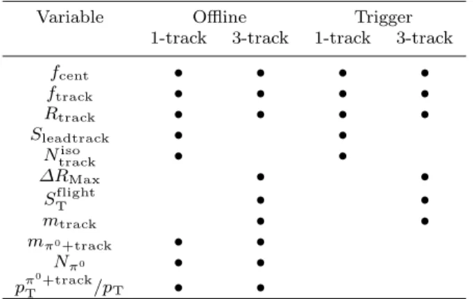
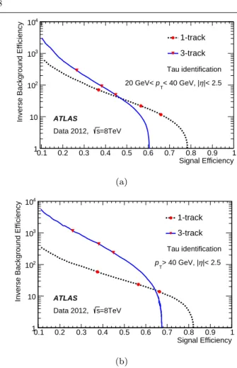
(7) The ATLAS Collaboration. Variable fcent ftrack Rtrack Sleadtrack iso Ntrack ∆RMax flight ST mtrack mπ0 +track Nπ 0 π 0 +track pT /pT. Offline 1-track 3-track • • • • •. • • •. • • • • • • • • •. Trigger 1-track 3-track • • • • •. • • • • • •. Table 2 Discriminating variables used as input to the tau identification algorithm at offline reconstruction and at trigger level, for 1-track and 3-track candidates. The bullets indicate whether a particular variable is used for a given selection. The π 0 -reconstruction-based variables, mπ0 +track , Nπ0 , 0 +track pπ /pT are not used in the trigger. T. The distributions of some of the important discriminating variables listed in Table 2 are shown in Figs. 2 and 3. Separate BDT algorithms are trained for 1-track and 3-track τhad-vis decays using a combination of simulated tau leptons in Z, W and Z ′ decays. For the jet background, large collision data samples collected by jet triggers, referred from now on as the multi-jet data samples, are used. For the signal, only reconstructed τhad-vis candidates matched to the true (i.e., generatorlevel) visible hadronic tau decay products in the region true around ∆R < 0.2 with ptrue T,vis > 10 GeV and |ηvis | < 2.3 are used. In the following, the signal efficiency is defined as the fraction of true visible hadronic tau decays. Z, Z’ → ττ, W → τν (Simulation). 0.25. Multi-Jet (Data 2012). 0.2. p > 15 GeV, |η |< 2.5 T. 0.15 0.1. 1-track. ATLAS. s = 8 TeV. 0.05 0 0. 0.2. 0.4. 0.6. 0.8. 1. f cent. (a) Arbitrary Units. structed from the tracks associated with the core region of the τhad-vis candidate) in the transverse plane, calculated with respect to the TV, divided by its estimated uncertainty. It is defined only for multi-track τhad-vis candidates. Track mass (mtrack ): Invariant mass calculated from the sum of the four-momentum of all tracks in the core and isolation regions, assuming a pion mass for each track. Track-plus-π 0 -system mass (mπ0 +track ): Invariant mass of the system composed of the tracks and π 0 mesons in the core region. Number of π 0 mesons (Nπ0 ): Number of π0 mesons reconstructed in the core region. π0 +track /pT ): Ratio of track-plus-π 0 -system pT (pT Ratio of the pT estimated using the track + π 0 information to the calorimeter-only measurement.. Arbitrary Units. 6. 1. ATLAS s = 8 TeV. 0.8. Z, Z’ → ττ, W → τν (Simulation) Multi-Jet (Data 2012). 0.6. p > 15 GeV, |η |< 2.5. 0.4. T. 1-track 0.2 0. 0. 1. 2. 3. 4. 5. 6. N iso track. (b) Fig. 2 Signal and background distribution for the 1-track τhad-vis decay offline tau identification variables (a) fcent iso and (b) Ntrack . For signal distributions, 1-track τhad-vis decays are matched to true generator-level τhad-vis in simulated events, while the multi-jet events are obtained from the data.. with n charged decay products, which are reconstructed with n associated tracks and satisfy tau identification criteria. The background efficiency is the fraction of reconstructed τhad-vis candidates with n associated tracks which satisfy tau identification criteria, measured in a background-dominated sample. Three working points, labelled tight, medium and loose, are provided, corresponding to different tau identification efficiency values. Their signal efficiency values (defined with respect to 1-track or 3-track reconstructed τhad-vis candidates matched to true τhad-vis ) can be seen in Fig. 4. The requirements on the BDT score are chosen such that the resulting efficiency is independent of the true τhad-vis pT . Due to the choice of input variables, the tau identification also shows stability with respect to the pile-up conditions as shown in Fig. 4. The performance of the tau identification algorithm in terms of the inverse background efficiency versus the signal efficiency is shown in Fig. 5. At low transverse.

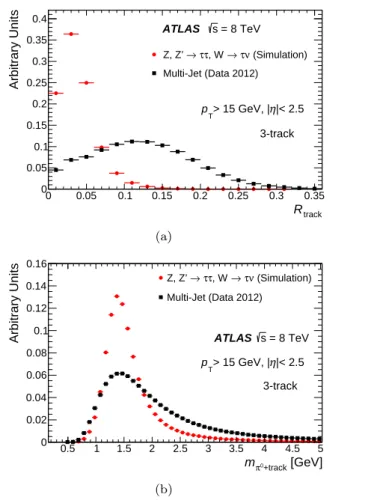
(8) 0.4. Signal Efficiency. Arbitrary Units. Identification and energy calibration of hadronically decaying tau leptons in ATLAS at. s = 8 TeV. ATLAS. 0.35 Z, Z’ → ττ, W → τν (Simulation). 0.3. Multi-Jet (Data 2012). 0.25 0.2. p > 15 GeV, |η |< 2.5. √. s=8 TeV. 7. 1.2 loose medium tight. 1. ATLAS Simulation, s=8 TeV p > 15 GeV, |η |< 2.5 T. 1-track. 0.8 0.6. T. 0.15. 0.4. 3-track. 0.1. 0.2. 0.05 0 0. 0.05. 0.1. 0.15. 0.2. 0.25. 0.3. 0. 0.35. 5. 10. R track. 20. 25. (a). 0.16. Signal Efficiency. Arbitrary Units. (a) Z, Z’ → ττ, W → τν (Simulation). 0.14. 15. Number of primary vertices. Multi-Jet (Data 2012). 0.12 0.1. ATLAS s = 8 TeV. 0.08. p > 15 GeV, |η |< 2.5. 1.2 ATLAS Simulation, s=8 TeV. loose medium tight. 1. p > 15 GeV, |η |< 2.5 T. 3-track. 0.8 0.6. T. 0.06. 0.4. 3-track 0.04. 0.2. 0.02 0. 0.5. 1. 1.5. 2. 2.5. 3. 3.5. 4. 4.5. 5. m π0+track [GeV]. 0. 5. 10. 15. 20. 25. Number of primary vertices. (b). (b). Fig. 3 Signal and background distribution for the 3-track τhad-vis decay offline tau identification variables (a) Rtrack and (b) mπ0 +track . For signal distributions, 3-track τhad-vis decays are matched to true generator-level τhad-vis in simulated events, while the multi-jet events are obtained from data.. Fig. 4 Offline tau identification efficiency dependence on the number of reconstructed interaction vertices, for (a) 1-track and (b) 3-track τhad-vis decays matched to true τhad-vis (with corresponding number of charged decay products) from SM and exotic processes in simulated data. Three working points, corresponding to different tau identification efficiency values, are shown.. momentum of the τhad-vis candidates, 40% signal efficiency for an inverse background efficiency of 60 is achieved. The signal efficiency saturation point, visible in these curves, stems from the reconstruction efficiency for a true τhad-vis with one or three charged decay products to be reconstructed as a 1-track or 3-track τhad-vis candidate. The main sources of inefficiency are track reconstruction efficiency due to hadronic interactions and migration of the number of reconstructed tracks due to conversions or underlying-event tracks being erroneously associated with the tau candidate.. 3.3 Tau trigger implementation The tau reconstruction at the trigger level has differences with respect to its offline counterpart due to the technical limitations of the trigger system. At L1, no inner detector track reconstruction is available, and the. full calorimeter granularity cannot be accessed. Latency limits at L2 prevent the use of the TopoCluster algorithm, and only allow the candidate reconstruction to be performed within the given RoI. At the EF, the same tau reconstruction and identification methods as offline are used, except for the π 0 reconstruction. In this section, the details of the tau trigger reconstruction algorithm are described. Level 1 At L1, the τhad-vis candidates are selected using calorimeter energy deposits. Two calorimeter regions are defined by the tau trigger for each candidate, using trigger towers in both the EM and HAD calorimeters: the core region, and an isolation region around this core. The trigger towers have a granularity of ∆η × ∆φ = 0.1 × 0.1 with a coverage of |η| < 2.5. The core region is defined as a square of 2 × 2 trigger towers, corresponding to 0.2 × 0.2 in ∆η × ∆φ space..

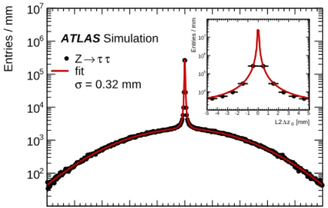
(9) The ATLAS Collaboration Inverse Background Efficiency. 8 104. 1-track 3. 3-track. 10. Tau identification 20 GeV< p < 40 GeV, |η |< 2.5. 102. 10. T. ATLAS Data 2012,. 1 0.1. 0.2. 0.3. s=8TeV. 0.4. 0.5. 0.6. 0.7. 0.8 0.9 1 Signal Efficiency. Inverse Background Efficiency. (a) 4. 10. 1-track 103. 3-track Tau identification p > 40 GeV, |η |< 2.5. 2. 10. 10. 1 0.1. T. ATLAS Data 2012,. s=8TeV. 0.2. 0.4. 0.3. 0.5. 0.6. 0.7. 0.8 0.9 1 Signal Efficiency. (b) Fig. 5 Inverse background efficiency versus signal efficiency for the offline tau identification, for (a) a low-pT and (b) a high-pT τhad-vis range. Simulation samples for signal include a mixture of Z, W and Z ′ production processes, while data from multi-jet events is used for background. The red markers correspond to the three working points mentioned in the text. The signal efficiency shown corresponds to the total efficiency of τhad-vis decays to be reconstructed as 1-track or 3-track and pass tau identification selection.. The ET of a τhad-vis candidate at L1 is taken as the sum of the transverse energy in the two most energetic neighbouring central towers in the EM calorimeter core region, and in the 2 × 2 towers in the HAD calorimeter, all calibrated at the EM scale. For each τhad-vis candidate, the EM isolation is calculated as the transverse energy deposited in the annulus between 0.2 × 0.2 and 0.4 × 0.4 in the EM calorimeter. To suppress background events and thus reduce trigger rates, an EM isolation energy of less than 4 GeV is required for the lowest ET threshold at L1. Hardware limitations prevent the use of an ET -dependent selection. This requirement reduces the efficiency of τhad-vis events by less than 2% over most of the kinematic range. Larger efficiency losses occur for τhad-vis events at high ET values; those are recovered through the use of trig-. gers with higher ET thresholds but without any isolation requirements. The energy resolution at L1 is significantly lower than at the offline level. This is due to the fact that all cells in a trigger tower are combined without the use of sophisticated clustering algorithms and without τhad-vis -specific energy calibrations. Also, the coarse energy and geometrical position granularity limits the precision of the measurement. These effects lead to a significant signal efficiency loss for low-ET τhad-vis candidates. Level 2 At L2, τhad-vis candidate RoIs from L1 are used as seeds to reconstruct both the calorimeter- and tracking-based observables associated with each τhad-vis candidate. The events are then selected based on an identification algorithm that uses these observables. The calorimeter observables associated with the τhad-vis candidates are calculated using calorimeter cells, where the electronic and pile-up noise are subtracted in the energy calibration. The centre of the τhad-vis energy deposit is taken as the energy-weighted sum of the cells collected in the region ∆R < 0.4 around the L1 seed. The transverse energy of the τhad-vis is calculated using only the cells in the region ∆R < 0.2 around its centre. To calculate the tracking-based observables, a fast tracking algorithm [48] is applied, using only hits from the pixel and SCT tracking layers. Only tracks satisfying pT > 1.5 GeV and located in the region ∆R < 0.3 around the L2 calorimeter τhad-vis direction are used. The tracking efficiency with respect to offline reaches a plateau of 99% at 2 GeV (with an efficiency of about 98% at 1.5 GeV). The fast tracking algorithm required an average of 37 ms to run at the highest pile-up conditions at peak luminosity in 2012 (approximately forty pile-up interactions). As there is no vertex information available at this stage, an alternative approach is used to reject tracks coming from pile-up interactions. A requirement is placed on the ∆z0 between a candidate track and the highest-pT track inside the RoI. The distribution of ∆z0 is shown in Fig. 6 for simulated Z → τ τ events with an average of eight interactions per bunch crossing. High values of ∆z0 typically correspond to pile-up tracks while the central peak corresponds to the main interaction tracks. The ∆z0 distribution is fit to the sum of a Breit– Wigner function to describe the central peak and a Gaussian function to describe the broad distribution from tracks in pile-up events. The half-width of the Breit–Wigner σ=0.32 mm is taken as the point where 68% of the signal events are included in the central peak. A dependence of the trigger variables on pile-.

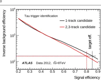
(10) Identification and energy calibration of hadronically decaying tau leptons in ATLAS at. up conditions is minimized by considering only tracks within −2 mm < ∆z0 < 2 mm and ∆R < 0.1 with respect to the highest-pT track. Track isolation requirements are applied to τhad-vis candidates to increase background rejection. For multitrack candidates (candidates with two or three associated tracks, defined to be as inclusive as possible with respect to their offline counterpart), the ratio of the sum of the track pT in 0.1 < ∆R < 0.3 to the sum of the track pT in ∆R < 0.1 is required to be lower than 0.1. Any 1-track candidate with a reconstructed track in the isolation region is rejected.. 107 106 5. 10. Entries / mm. Entries / mm. In the last step, identification variables combining calorimeter and track information are built as described in Sect. 3.2. The calorimeter-based isolation variable fcent uses an expanded cone size of ∆R < 0.4 without the pile-up correction term to estimate the fraction of transverse energy deposited in the region ∆R < 0.1 around the τhad-vis candidate. The variables ftrack and Rtrack , measuring respectively the ratio of the transverse momentum of the leading pT track to the total transverse energy (calibrated at the EM energy scale) and the pT -weighted distance of the associated tracks to the τhad-vis direction, are calculated using selected tracks in the region ∆R < 0.3 around the highest-pT track. Cuts on the chosen identification variables are optimized to provide an inverse background efficiency of roughly ten while keeping the signal efficiency as high as possible (approximately 90% with respect to the offline medium tau identification).. ATLAS Simulation Z→ τ τ fit σ = 0.32 mm. 107 6. 10. 5. 10. 104. 104. -5. -4. -3. -2. -1. 0. 1. 2. 3. 4. 5. L2 ∆ z 0 [mm]. 103 102 -250 -200 -150 -100 -50. 0. 50 100 150 200 250 L2 ∆z 0 [mm]. Fig. 6 Distribution of ∆z0 for the tau trigger at L2 in simulated Z → τ τ events with an average of eight interactions per bunch crossing. The wide Gaussian distribution corresponds to pile-up tracks while the central peak, displayed in the upper-right corner, corresponds to the main interaction tracks. A Breit–Wigner function is fitted to the central peak and 68% of the signal events are found within a distance σ = 0.32 mm from the peak.. √. s=8 TeV. 9. Event Filter At the EF level, the τhad-vis reconstruction is very similar to the offline version. First, the TopoCluster reconstruction and calibration algorithms are run within the RoI. Then, track reconstruction inside the RoI is performed using the EF tracking algorithm. In the last step, the full offline τhad-vis reconstruction algorithm is used. The EF tracking is almost 100% efficient over the entire pT range with respect to the offline reconstructed tracks. It is, however, considerably slower than the L2 fast tracking algorithm, requiring about 200 ms per RoI under severe pile-up conditions (forty pile-up interactions). The TopoClustering algorithms need only about 15 ms. The τhad-vis candidate four-momentum and input variables to the EF tau identification are then calculated. The main difference with respect to the offline tau reconstruction is that π 0 -reconstruction-based inπ 0 +track put variables (mπ0 +track , Nπ0 and pT /pT ) are not used; the methodology to compute these variables had not yet been developed when the trigger was implemented. Furthermore, no pile-up correction is applied to the input variables at trigger level. Since full-event vertex reconstruction is not available at trigger level (vertices are only formed using the tracks in a given RoI), the selection requirements applied to the input tracks are also different with respect to the offline τhad-vis reconstruction. Similarly to L2, the ∆z0 requirement for tracks is computed with respect to the leading track, and loosened to 1.5 mm with respect to the offline requirement. The ∆d0 requirement is calculated with respect to the vertex found inside of the RoI, and is loosened to 2 mm. A BDT with the input variables listed in Table 2 is used to suppress the backgrounds from jets misidentified as τhad-vis . The BDT was trained on 1- and 3-track τhad-vis candidates with simulated Z, W and Z ′ events for the signal and data multi-jet samples for the background, respectively. Only events passing an L1 tau trigger matched with an offline reconstructed τhad-vis with pT > 15 GeV and |η| < 2.2 are used, where the medium identification is required for the τhad-vis candidates. For the signal, in addition, a geometrical matching to a true τhad-vis is required. The performance of the EF tau trigger is presented in Fig. 7. The signal efficiency is defined with respect to offline reconstructed τhad-vis candidates matched at generator level, and the inverse background efficiency is calculated in a multijet sample. The working points are chosen to obtain a signal efficiency of 85% and 80% with respect to the offline medium candidates for 1-track and multi-track candidates respectively, where the inverse background efficiency is of the order of 200 for the multi-jet sample..

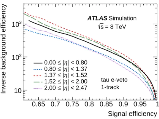
(11) The ATLAS Collaboration. Tau trigger identification. 1-track candidate 2,3-track candidate. 103. 102. ATLAS. 0.2. 0.3. Data 2012,. 0.4. s=8TeV. 0.5. 0.6. 0.7. 0.8. 0.9. Signal efficiency. the reasons for this is that the variable associated with transition radiation (the leading track’s ratio of highthreshold TRT hits to low-threshold TRT hits) is not available for |η| > 2.0. Three working points, labelled tight, medium and loose are chosen to yield signal efficiencies of 75%, 85%, and 95%, respectively.. Arbitrary Units. 104. target eff.. Inverse background efficiency. 10. Fig. 7 Inverse background efficiency versus signal efficiency for the tau trigger at the EF level, for τhad-vis candidates which have satisfied the L1 requirements. The signal efficiency is defined with respect to offline medium tau identification τhad-vis candidates matched at generator level, and the inverse background efficiency is calculated in a multi-jet sample.. 0.25. Z → ττ Z → ee. 0.2. ATLAS Simulation, s = 8 TeV. 0.1 0.05 0 0 0.05 0.1 0.15 0.2 0.25 0.3 0.35 0.4 0.45 0.5 f HT (a). Arbitrary Units. Electron veto The characteristic signature of 1-track τhad-vis can be mimicked by electrons. This creates a significant background contribution after all the jet-related backgrounds are suppressed via kinematic, topological and τhad-vis identification criteria. Despite the similarities of the τhad-vis and electron signatures, there are several properties that can be used to discriminate between them: transition radiation, which is more likely to be emitted by an electron and causes a higher ratio fHT of high-threshold to low-threshold track hits in the TRT for an electron than for a pion; the angular distance of the track from the τhad-vis calorimeterbased direction; the ratio fEM of energy deposited in the EM calorimeter to energy deposited in the EM and HAD calorimeters; the amount of energy leaking into the hadronic calorimeter (longitudinal shower information) and the ratio of energy deposited in the region 0.1 < ∆R < 0.2 to the total core region ∆R < 0.2 (transverse shower information). The distributions for two of the most powerful discriminating variables are shown in Fig. 8. These properties are used to define a τhad-vis identification algorithm specialized in the rejection of electrons misidentified as hadronically decaying tau leptons, using a BDT. The performance of this electron veto algorithm is shown in Fig. 9. Slightly different sets of variables are used in different η regions. One of. T. 0.15. 3.4 Discrimination against electrons and muons Additional dedicated algorithms are used to discriminate τhad-vis from electrons and muons. These algorithms are only used offline.. 1-track p > 15 GeV, |η| < 2.0. 0.5 Z → ττ Z → ee. 0.4. 1-track p > 15 GeV, |η| < 2.5 T. ATLAS. 0.3. Simulation,. s = 8 TeV. 0.2 0.1 0. 0. 0.2. 0.4. 0.6. 0.8. 1 f EM. (b) Fig. 8 Signal and background distribution for two of the electron veto variables, (a) fHT and (b) fEM . Candidate 1track τhad-vis decays are required to not overlap with a reconstructed electron candidate which passes tight electron identification [23]. For signal distributions, 1-track τhad-vis decays are matched to true generator-level τhad-vis in simulated Z → τ τ events, while the electron contribution is obtained from simulated Z → ee events where 1-track τhad-vis decays are matched to true generator-level electrons.. Muon veto Tau candidates corresponding to muons can in general be discarded based on the standard muon identification algorithms [24]. The remaining contamination level can typically be reduced to a negligible level by a cut-based selection using the following char-.

(12) Inverse background efficiency. Identification and energy calibration of hadronically decaying tau leptons in ATLAS at. ATLAS Simulation s = 8 TeV. 103. 102. 10. 0.00 0.80 1.37 1.52 2.00. ≤ |η | < 0.80 ≤ |η | < 1.37 ≤ |η | < 1.52 ≤ |η | < 2.00 ≤ |η | < 2.47. tau e-veto 1-track. 0.65 0.7 0.75 0.8 0.85 0.9 0.95 1 Signal efficiency Fig. 9 Electron veto inverse background efficiency versus signal efficiency in simulated samples, for 1-track τhad-vis candidates. The background efficiency is determined using simulated Z → ee events.. acteristics. Muons are unlikely to deposit enough energy in the calorimeters to be reconstructed as τhad-vis candidates. However, when a sufficiently energetic cluster in the calorimeter is associated with a muon, the muon track and the calorimeter cluster together may be misidentified as a τhad-vis . Muons which deposit a large amount of energy in the calorimeter and therefore fail muon spectrometer reconstruction are characterized by a low electromagnetic energy fraction and a large ratio of track-pT to ET deposited in the calorimeter. Lowmomentum muons which stop in the calorimeter and overlap with calorimeter deposits of different origin are characterized by a large electromagnetic energy fraction and a low pT -to-ET ratio. A simple cut-based selection based on these two variables reduces the muon contamination to a negligible level. The resulting efficiency is better than 96% for true τhad-vis , with a reduction of muons misidentified as τhad-vis of about 40%. However, the performance can vary depending on the τhad-vis and muon identification levels.. 4 Efficiency measurements using Z tag-and-probe data. √. s=8 TeV. 11. (tag) and containing a hadronically decaying tau lepton candidate (probe) in the final state and extracting the efficiencies directly from the number of reconstructed τhad-vis before and after tau identification algorithms are applied. In practice, it is impossible to obtain a pure sample of hadronically decaying tau leptons, or electrons misidentified as a tau signal, and therefore backgrounds have to be taken into account. This is described in the following sections. 4.1 Offline tau identification efficiency measurement To estimate the number of background events for the purpose of tau identification efficiency measurements, a variable with high separation power, which is modelled well for simulated τhad-vis decays is chosen: the sum of the number of core and outer tracks associated to the τhad-vis candidate. Outer tracks in 0.2 < ∆R < 0.6 are only considered if they fulfill the requirement outer Douter = min([ pcore ] · ∆R(core, outer)) < 4, T /pT core where pT refers to any track in the core region, and ∆R(core, outer) refers to the distance between the candidate outer track and any track in the core region. This requirement suppresses the contribution of outer tracks from underlying and pile-up events, due to requirements on the relative momentum and separation of the tracks. This allows the signal track multiplicity to retain the same structure as the core track multiplicity distribution. For backgrounds from multi-jet events, the track multiplicity is increased by the addition of tracks with significant momentum in the outer cone. The requirement on Douter was chosen to offer optimal signal to background separation. A fit is then performed using the expected distributions of this variable for both signal and background to extract the τhad-vis signal. This fit is performed for each exclusive tau identification working point, corresponding to: candidates failing the loose requirement, candidates satisfying the loose requirement but failing the medium requirement, candidates satisfying the medium requirement but failing the tight requirement and candidates satisfying the tight requirement. 4.1.1 Event selection. To perform physics analyses it is important to measure the efficiency of the reconstruction and identification algorithms used online and offline with collision data. For the τhad-vis signal, this is done on a sample enriched in Z → τ τ events. For electrons misidentified as a tau signal (after applying the electron veto) this is done on a sample enriched in Z → ee events. The chosen tag-and-probe approach consists of selecting events triggered by the presence of a lepton. Z → τlep τhad events are selected by a triggered muon or electron coming from the leptonic decay of a tau lepton, and the hadronically decaying tau lepton is then searched for in the rest of the event, considered as the probe for the tau identification performance measurement. These events are triggered by a single-muon or a single-electron trigger requiring one isolated trigger muon or electron with a pT of at least 24 GeV..

(13) 12. Offline, muons and electrons with pT > 26 GeV are thereafter selected, representing the tag objects. Additional track and calorimeter isolation requirements are applied to the muon and electron. Identified muons are required to have |η| < 2.4. Identified electrons are required to have |η| < 1.37 or 1.52 < |η| < 2.47, therefore excluding the poorly instrumented region at the interface between the barrel and endcap calorimeters. In addition to the requirement of exactly one isolated muon or electron (ℓ), a τhad-vis candidate is selected in the kinematic range pT > 15 GeV and |η| < 2.5, requiring one or three associated tracks in the core region and an absolute electric charge of one and no geometrical overlap with muons with pT > 4 GeV or with electrons with pT > 15 GeV of loose or medium quality (depending on η). For τhad-vis with one associated track, a muon veto and a medium electron veto is applied. In addition to this, a very loose requirement on the tau identification BDT score is made which strongly suppresses jets while being more than 99% efficient for Z → τ τ signal. The tag and the probe objects are required to have opposite-sign electric charges (OS). Additional requirements are made in order to suppress (Z → ℓℓ) + jets and (W → ℓνℓ ) + jets events: – On the invariant mass calculated from the lepton and the τhad-vis four-momenta (mvis (ℓ, τhad-vis )): for pτThad-vis < 20 GeV, 45 GeV < mvis (ℓ, τhad-vis ) < 80 GeV. Otherwise, for the µ channel, 50 GeV < mvis (µ, τhad-vis ) < 85 GeV, and for the e channel: 50 GeV < mvis (e, τhad-vis ) < 80 GeV. For the signal, this variable peaks in these regions. miss – On the transverse q mass of the lepton and ET. miss (1 − cos ∆φ(ℓ, E miss ))): system (mT = 2pℓT · ET T mT < 50 GeV. For most backgrounds (e.g. (W → ℓνℓ ) + jets), this variable peaks at larger values. – On the distance in the azimuthal plane between miss the lepton and ET (neutrinos) and between the miss miss τhad-vis and ET (Σ cos ∆φ = cos ∆φ(ℓ, ET )+ miss cos ∆φ(τhad-vis , ET )): Σ cos ∆φ > −0.15. For the signal, this variable tends to peak at zero, indicating that the neutrinos point mainly in the direction of one of the two leptons from Z decay products. For W + jets background events, the value is typically negative, indicating that the neutrino points away from the two lepton candidates.. 4.1.2 Background estimates and templates The signal track multiplicity distribution is modelled using simulated Z → τlep τhad events. Only reconstructed τhad-vis matched to a true hadronic tau decay are considered.. The ATLAS Collaboration. A single template is used to model the background from quark- and gluon-initiated jets that are misidentified as hadronic tau decays. The background is mainly composed of multi-jet and W +jets events with a minor contribution from Z+jets events. The template is constructed starting from a enriched multi-jet control region in data that uses the full signal region selection but requires that the tag and probe objects have samesign charges (SS). The contributions from W +jets and Z+jets in the SS control region are subtracted. The template is then scaled by the ratio of OS/SS multijet events, measured in a control region which inverts the very loose identification requirement of the signal region. Finally, the OS contributions from W +jets and Z+jets are added to complete the template. The Z+jets contribution is estimated using simulated samples. The shape of the W +jets contribution is estimated from a high-purity W +jets control region, defined by removing the mT requirement and inverting the requirement on Σ cos ∆φ. The normalization of the W +jets contribution is estimated using simulation. An additional background shape is used to take into account the contamination due to misidentified electrons or muons. This small background contribution (stemming mainly from Z → ℓℓ events) is modelled by taking the shape predicted by simulation using candidates which are not matched to true τhad-vis in events of type Z → τlep τhad , tt̄, diboson, Z → ee, µµ where the reconstructed tau candidate probe is matched to a electron or muon. For the fit, the contribution of these backgrounds is fixed to the value predicted by the simulation, which is typically less than 5% of the total signal yield. To measure both the 1-track and 3-tracks τhad-vis efficiencies, a fit of the data to the model (signal plus background) is performed, using two separate signal templates. The signal templates are obtained by requiring exactly one or three tracks reconstructed in the core region of the τhad-vis candidate. To improve the fit stability in the background-dominated region where the tau candidates fail the loose requirements, the ratio of the 1-track to 3-track normalization is fixed to the value predicted by the simulation. For other exclusive regions, the ratio is allowed to vary during the fit. In the fit to extract the efficiencies for real tau leptons passing different levels of identification, the ratio of jet to other τhad-vis candidates is determined in a preselection step (where no identification is required) and then extrapolated to regions where identification is required by using jet misidentification rates determined in an independent data sample..

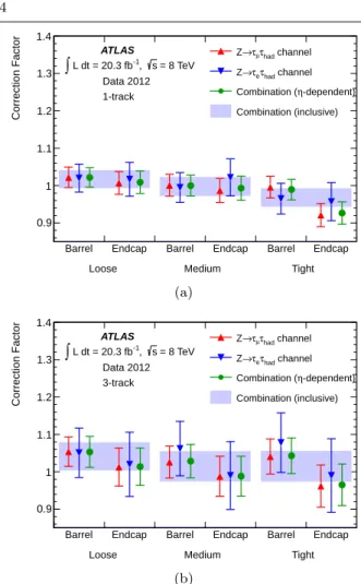
(14) Figure 10 shows an example of the track multiplicity distribution after the tag-and-probe selection, before and after applying the tau identification requirements, with the results of the fit performed. The peaks in the one- and three-track bins are due to the signal contribution. These are visible before any identification requirements are applied, and become considerably more prominent after identification requirements are applied, due to the large amount of background rejection provided by the identification algorithm. To account for the small differences between data and simulations, correction factors, defined as the ratio of the efficiency in data to the efficiency in simulation for τhad-vis signal to pass a certain level of identification, are derived. Their values are compatible with one, except for the tight 1-track working point, where the correction factor is about 0.9.. √. s=8 TeV. 13. 50000 ATLAS. 40000. ∫ Ldt = 20.3 fb , Zs→= τ8 TeV τ. 30000. Data 2012. -1. µ had. Fit 1-track τ. 20000. 3-track τ Jets Electrons. 10000 0. 0. 1. 2. 3. 4. 5. 6. 7. 8. 9 10 11 12 Number of tracks. (a) Events. 4.1.3 Results. Events. Identification and energy calibration of hadronically decaying tau leptons in ATLAS at. 30000. ∫. 25000. ATLAS -1. Ldt = 20.3 fb , s = 8 TeV Z →τ µ τ had. 20000. Data 2012. Results from the electron- and muon-tag analysis are combined to improve the precision of the correction factors, shown in Fig. 11. No significant dependency on the pT of the τhad-vis is observed and hence the results are provided separately only for the barrel (|η| < 1.5) and the endcap (1.5 < |η| < 2.5) region, and for one and three associated tracks. Uncertainties depend slightly on the tau identification level and kinematic quantities. In Table 3, the most important systematic uncertainties for the working point used by most analyses, medium tau identification, are shown, together with the total statistical and systematic uncertainty. Uncertainties due to the underlying event (UE) are the dominant ones for the signal template, and are estimated by comparing alpgen-Herwig and Pythia simulations. The shower model and the amount of detector material are also varied and included in the number reported in Table 3. The W +jets shape uncertainty accounts for differences between the W +jets shape in the signal and control regions and is derived from comparisons to simulated W +jets events. The jet background fraction uncertainty accounts for the effect of propagating the statistical uncertainty on the jet misidentification rates. The results apply to τhad-vis candidates with pT > 20 GeV. For pT < 20 GeV, uncertainties increase to a maximum of 15% for inclusive τhad-vis candidates. For pT > 100 GeV, there are no abundant sources of hadronic tau decays to allow for an efficiency measurement. Previous studies using high-pT dijet events indicate that there is no degradation in the modelling of tau identification in this pT range, within the statistical uncertainty of the measurement [14].. Fit. 15000. 1-track τ 3-track τ. 10000. Jets Electrons. 5000 0. 0. 1. 2. 3. 4. 5. 6. 7 8 9 Number of tracks. (b) Fig. 10 Template fit result in the muon channel, inclusive in η and pT for pT > 20 GeV for the offline τhad-vis candidates (a) before the requirement of tau identification, and (b) fulfilling the medium tau identification requirement.. Source. Uncertainty [%] 1-track 3-track. Jet background fraction Jet template shape Tau energy scale Shower model/UE Statistics. 0.8 0.9 0.7 1.8 1.0. 1.5 1.4 0.8 2.5 2.2. Total. 2.5. 4.0. Table 3 Dominant uncertainties on the medium tau identification efficiency correction factors estimated with the Z tagand-probe method, and the total uncertainty, which combines systematic and statistical uncertainties. These uncertainties apply to τhad-vis candidates with pT > 20 GeV..

(15) The ATLAS Collaboration Correction Factor. 14 1.4 1.3. ∫. Z→τµτhad channel. ATLAS L dt = 20.3 fb-1, s = 8 TeV. Z→τeτhad channel. Data 2012 1-track. Combination (η-dependent). 1.2. Combination (inclusive). 1.1. 1 0.9 Barrel. Endcap. Loose. Barrel. Endcap. Medium. Barrel. Endcap. Tight. Correction Factor. (a) 1.4 Z→τµτhad channel. ATLAS. 1.3. ∫ L dt = 20.3 fb-1,. s = 8 TeV. Z→τeτhad channel. Data 2012 3-track. Combination (η-dependent). 1.2. Combination (inclusive). 1.1. 1 0.9 Barrel. Endcap. Loose. Barrel. Endcap. Medium. Barrel. Endcap. Tight. (b) Fig. 11 Correction factors needed to bring the offline tau identification efficiency in simulation to the level observed in data, for all tau identification working points as a function of η. The combinations of the muon and electron channels are also shown, and the results are displayed separately for (a) 1-track and (b) 3-track τhad-vis candidates with pT > 20 GeV. The combined systematic and statistical uncertainties are shown.. 4.2 Trigger efficiency measurement The tau trigger efficiency is measured with Z → τ τ events using tag-and-probe selection similar to the one described in Sect. 4.1. The only difference is that the efficiency is measured with respect to identified offline τhad-vis candidates and thus, offline tau identification selection criteria are applied during the event selection. Only the muon channel is considered, as the background contamination is smaller than in the electron channel. The statistical uncertainty improvements that could be obtained by the addition of the electron channel are offset by the larger systematic uncertainties associated with this channel. The systematic uncertainties are also different from those in the offline identification measurement, since the purity after identification is already. high. The systematics are dominated by the uncertainties on the modelling of the kinematics of the background events, rather than the total normalization, as is the case for the offline identification measurement. The dominant background contribution is due to W + jets and multi-jet events, where a jet is misidentified as a τhad-vis . These backgrounds are estimated using a method similar to the one described in Sect. 4.1.2. The same multi-jet and W + jets control regions are used. The shape of other backgrounds is taken from simulation but the normalizations of the dominant backgrounds are estimated from data control regions. The contribution of top quark events is normalized in a control region requiring one jet originating from a b-quark. Z+jets events with leptonic Z decays and one of the additional jets being misidentified as τhad-vis are normalized by measuring this misidentification rate in a control region with two identified oppositely charged same-flavour leptons. In total, more than 60,000 events are collected, with a purity of about 80% when the offline medium tau identification requirement is applied. With the addition of the tau trigger requirement, the purity increases to about 88%. Most of the backgrounds accumulate in the region pT < 30 GeV. Figure 12 shows the measured tau trigger efficiency for τhad-vis candidates identified by the offline medium tau identification as functions of the offline τhad-vis transverse energy and the number of primary vertices in the event, for each level of the trigger. The tau trigger considered has calorimetric isolation and a pT threshold of 11 GeV at L1, a 20 GeV requirement on pT , the number of tracks restricted to three or less, and medium selection on the BDT score at EF. The efficiency depends minimally on pT for pT > 35 GeV or on the pile-up conditions. The measured tau trigger efficiency is compared to simulation in Fig. 13; the efficiency is shown to be modelled well in simulation. Correction factors, as defined in Sect. 4.1, are derived from this measurement. The correction factors are in general compatible with unity, except for the region pT < 40 GeV where a difference of a few per cent is observed. In the pT range from 30 GeV to 50 GeV, the uncertainty on the correction factors is about 2% but increases to about 8% for pT = 100 GeV. The uncertainty is also sizeable in the region pT < 30 GeV, where the background contamination is the largest. 4.3 Electron veto efficiency measurement To measure the efficiency for electrons reconstructed as τhad-vis to pass the electron veto in data, a tag-andprobe analysis singles out a pure sample of Z → ee.

(16) Efficiency. Efficiency. Identification and energy calibration of hadronically decaying tau leptons in ATLAS at 1 0.8 0.6. ATLAS. ∫ Ldt = 20.3 fb , -1. L1. Data 2012, Z → τ µ τ had. L1 + L2. 0.2 0 0. 20 GeV tau trigger. L1 + L2 + EF. 20. 40. s = 8 TeV. 60. 80. 100. Offline tau p T [GeV]. Efficiency. (a). εData/εSim.. 0.4. 1 0.9 0.8 0.7 0.6 0.5 0.4 0.3 0.2 0.1 0 1.2 1.1 1 0.9 0.8 0. √. s=8 TeV. ATLAS. ∫ Ldt = 20.3 fb. -1. s = 8 TeV Z → τ µ τ had. Sim. Z → τ τ. Data stat. error. Sim. stat. error. Data sys. error. Stat. (Data) Stat. (Sim.) Sys.. 20. 40. 0.6. ATLAS. ∫ Ldt = 20.3 fb , -1. 0.2 0 0. 80 100 Offline tau p T [GeV]. 20 GeV tau trigger. L1 + L2 + EF. 5. s = 8 TeV. Data 2012, Z → τ µ τ had. L1 + L2. 60. Fig. 13 The measured tau trigger efficiency in data and simulation, for the offline τhad-vis candidates passing the medium tau identification, as a function of offline τhad-vis transverse energy. The expected background contribution has been subtracted from the data. The uncertainty band on the ratio reflects the statistical uncertainties associated with data and simulation and the systematic uncertainty associated with the background subtraction in data.. 0.8. L1. 20 GeV tau trigger. Data 2012. 1. 0.4. 15. 10. 15. 20. 25. (b). bution is obtained from simulation but normalized to dedicated data control regions for each background.. Fig. 12 The tau trigger efficiency for τhad-vis candidates identified by the offline medium tau identification, as a function of (a) the offline τhad-vis transverse energy and (b) the number of primary vertices. The error bars correspond to the statistical uncertainty in the efficiency.. Differences in the modelling of the electron veto algorithm’s performance in simulation compared to data are parameterized as correction factors in bins of η of the τhad-vis candidate, by comparing distributions similar to the one shown in Fig. 14 (b).. Number of primary vertices. events, as illustrated in Fig. 14 (a). The measurement uses probe 1-track τhad-vis candidates in the opposite hemisphere to the identified tag electron. The tag electron is required to fulfil ptag T > 35 GeV in order to suppress backgrounds from Z → τ τ events. The probe is required not to overlap geometrically with an identified electron, e.g. in the case of Fig. 14 a loose electron identification is used. Different veto algorithms are tested in combination with different levels of jet discrimination, and the effects estimated. Efficiencies are extracted directly from the number of reconstructed τhad-vis before and after identification, in bins of η of the τhad-vis candidate, after subtracting the background modelled by simulation (normalized to data in dedicated control regions). The shape and normalization of the multi-jet background distribution for the η of the τhad-vis are estimated using events with SS tag electron and probe τhad-vis in data after subtracting backgrounds in the SS region using simulation. To estimate the W → eν, Z → τ τ , and tt̄ backgrounds, the shape of this distri-. Uncertainties on the correction factors (which are typically close to unity) are η-dependent and amount to about 10% for the loose electron veto and get larger for the medium and tight electron veto working points, mainly driven by statistical uncertainties. A summary of the main uncertainties for the working point shown in Fig. 14 is provided in Table 4.. Source. Uncertainty [%]. Tag selection (pT , isolation) Background rejection Statistics. 5–28 1–8 7–12. Total. 8–30. Table 4 Dominant uncertainties on the loose electron veto efficiency correction factors estimated with the Z tag-andprobe method. The range of the uncertainties reflects their variation with η..

(17) Events / 2 GeV. 16. The ATLAS Collaboration. 50000. ATLAS s = 8 TeV. 40000. Data 2012. W → eν. Z → ee. other. ∫ Ldt = 20.3 fb-1 5.1 Offline τhad-vis energy calibration. 30000 20000 10000 0 60. 70. 80. 90. 100. 110. 120 130 mvis [GeV]. Taus / 0.2. (a). 1200 ATLAS. 1000 800. s = 8 TeV. Data 2012. W → eν. Z → ee. other. ∫ Ldt = 20.3 fb-1. 600 400 200 0 -3. constructed and true TES or the modelling of the TES in simulation is more important.. -2. -1. 0. 1. 2. 3 ηtrack. (b) Fig. 14 (a) Visible mass of electron–positron pairs for the offline electron veto efficiency measurement, after tag-andprobe selection, where the probe lepton passes medium tau identification and does not overlap with loose electrons, before the electron veto is applied. (b) η distribution for τhad-vis candidates (electrons misidentified as hadronic tau decays) after applying a loose electron veto. Uncertainties shown are only statistical.. 5 Calibration of the τhad-vis energy The τhad-vis energy calibration is done in several steps. First, a calibration described in Sect. 5.1 and derived from simulation brings the tau energy scale (TES) into agreement with the true energy scale at the level of a few per cent and removes any significant dependencies of the energy scale on the pseudorapidity, energy, pile-up conditions and track multiplicity. Then, additional small corrections to the TES are derived using one of two independent data-driven methods described in Sect. 5.2. Which of the two methods is used depends on whether for a given study the agreement between re-. The clusters associated with the τhad-vis reconstruction are calibrated at the LC scale. For anti-kt jets with a distance parameter R = 0.4, this calibration accounts for the non-compensating nature of the ATLAS calorimeters and for energy deposited outside the reconstructed clusters and in non-sensitive regions of the calorimeters. However, it is neither optimized for the cone size used to measure the τhad-vis momentum (∆R = 0.2) nor for the specific mix of hadrons observed in tau decays; and it does not correct for the underlying event or for pile-up contributions. Thus an additional correction is needed to obtain an energy scale which is in agreement with the true visible energy scale, thereby also improving the τhad-vis energy resolution. This correction (also referred to as a response curve) τ is computed as a function of ELC using Z → τ τ , W → ′ τ ν and Z → τ τ events simulated with Pythia8. Only τhad-vis candidates with reconstructed ET > 15 GeV true and |η| < 2.4 matched to a true τhad-vis with ET,vis > 10 GeV are considered. Additionally, they are required to satisfy medium tau identification criteria and to have a distance ∆R > 0.5 to other reconstructed jets. The response is defined as the ratio of the reconstructed τ τhad-vis energy at the LC scale ELC to the true visible true energy Evis . The calibration is performed in two steps: first, the response curve is computed; then, additional small corrections for the pseudorapidity bias and for pile-up effects are derived. true The response curve is evaluated in intervals of Evis and of the absolute value of the reconstructed τhad-vis pseudorapidity for τhad-vis candidates with one or more tracks. In each interval, the distribution of this ratio is fitted with a Gaussian function to determine the mean value. This mean value as a function of the average τ ELC in a given interval is then fitted with an empirically derived functional form. The resulting functions are shown in Fig. 15. After using this response curve to calibrate hadronically decaying tau leptons their reconstructed mean energy is within 2% of the final scale, which is set using two additional small corrections. First, a pseudorapidity correction is applied, which is necessary to counter a bias due to underestimated reconstructed cluster energies in poorly instrumented regions. The correction depends only on |η LC | and is smaller than 0.01 units in the transition region between the barrel and end-.

(18) τ true E LC / Evis. Identification and energy calibration of hadronically decaying tau leptons in ATLAS at. √. s=8 TeV. 17. duces to about 5% for energies above a few hundred GeV. The resolution is worst in the transition region 1.3 < |η| < 1.6.. 1.1. 1.05. 0.95 0.9. | η | < 0.3 0.3 < |η | < 0.8 0.8 < |η | < 1.3 1.3 < |η | < 1.6 1.6 < |η | < 2.4. ATLAS Simulation 1−track. 0.85 0.8 20. 30 40. 102. 2×102. E. τ LC. 103 [GeV]. true σ(E reco - E true [%] vis )/ E vis. 1. τ true E LC / Evis. (a). 25. ATLAS 20. | η | < 0.3 0.3 < |η | < 0.8 0.8 0.8< <|η|| < 1.3 1.3 < |η | < 1.6 1.6 < |η | < 2.4. Simulation, 1−track. 15 10 5. 1.1. ATLAS Simulation. 1.05. 0. 100. 200. 300. 400. 500. 2,3−track. 600 true. E vis. 700 [GeV]. (a). 0.95 | η | < 0.3 0.3 < |η | < 0.8 0.8 < |η | < 1.3 1.3 < |η | < 1.6 1.6 < |η | < 2.4. 0.9 0.85 0.8 20. 30 40. 102. 2×102. 103 τ E LC [GeV]. (b) Fig. 15 Offline τhad-vis energy response curves as a funcτ tion of the reconstructed τhad-vis energy ELC for hadronic tau decays with (a) one and (b) more than one associated tracks. One curve per pseudorapidity region |η LC | is shown. The region where markers are shown corresponds approxiτ mately to a transverse energy ET,LC > 15 GeV. For very low and very high energies, the response curves are assumed to be constant. Uncertainties are statistical only.. cap electromagnetic calorimeters and negligible elsewhere, leading to the final reconstructed pseudorapidity η rec = η LC − η bias . Pile-up causes response variations of typically a few per cent. This is corrected by subtracting an amount of energy which is proportional to the number of reconstructed proton–proton interaction vertices nvtx in a given event. The parameter describing the proportionality is derived for different regions of |η rec | using a linear fit versus nvtx , for τhad-vis candidates with one or more tracks. The correction varies in the range 90–420 MeV per reconstructed vertex, increasing with |η|. The energy resolution, as determined from simulated data, as a function of the true visible energy after the complete tau calibration is shown in Fig. 16. The resolution is about 20% at very low E and re-. true σ(E reco - E true [%] vis )/ E vis. 1 25. ATLAS 20. | η | < 0.3 0.3 < |η | < 0.8 0.8 0.8< <|η|| < 1.3 1.3 < |η | < 1.6 1.6 < |η | < 2.4. Simulation, 3−track. 15 10 5 0. 100. 200. 300. 400. 500. 600. 700. E true [GeV] vis. (b) Fig. 16 Offline energy resolution for hadronically decaying tau leptons, separately for (a) one and (b) three associated tracks and for different pseudorapidity regions. The resolution shown is the standard deviation of a Gaussian function fit to true true the distribution of (Ereco − Evis )/Evis in a given range of true true Evis and |ηvis |.. 5.2 Additional offline tau calibration corrections and systematic uncertainties The systematic uncertainties on the tau energy scale are evaluated with two complementary methods. The deconvolution method gives access to uncertainties on both the absolute TES (differences between reconstructed and true visible energy) and the modelling (differences between data and simulation) and is based on dedicated measurements (such as test beam data and low-luminosity runs) and simulation. The in-situ.