Properties of submillimetre galaxies in a semi analytic model using the 'Count Matching' approach: application to the ECDF S
21
0
0
Texto completo
(2) 2. A. M. Muñoz Arancibia et al.. lines (Tacconi et al. 2006, Smolčić et al. 2012, Weiss et al. 2013, Hodge et al. 2013, Hatsukade et al. 2013, Chen et al. 2014, among others). Identification of counterparts at other wavelengths for different samples of SMGs has been carried out, either through deep optical/near infrared (NIR) spectroscopy or deep intermediate/high resolution radio imaging. This allows the spectroscopic follow-up of SMGs, as well as multiwavelength studies. The largest sample of SMGs with spectroscopic follow-up to date was obtained by Chapman et al. (2005), who measured a median spectroscopic redshift of 2.2 for 73 SMGs belonging to several fields, having a median 850 µ m flux density of 5.7 mJy. Moreover, using multiwavelength data Wardlow et al. (2011) derived a median photometric redshift of 2.2 ± 0.1 for 78 single-dish detected SMGs in the Extended Chandra Deep Field South (ECDF-S) over ∼ 4 mJy at 870 µ m. More recent studies have been successful identifying counterparts of single-dish detected SMGs using interferometers at millimeter (mm) wavebands. For instance, Smolčić et al. (2012) performed interferometric observations at 1.3 mm of SMGs in the central region of the Cosmic Evolution Survey (COSMOS) field, which had been discovered through single-dish observations at 870 µ m down to a signal-to-noise ratio (S/N) of 3.8; complementing this with additional multiwavelength catalogs, they derived a mean photometric redshift of 2.6 ± 0.4 for 16 of these SMGs. Having redshift information and multiwavelength photometry allows the performance of spectral energy distribution (SED) fitting, and then deriving other SMG properties as stellar mass and star formation rate (SFR). From several studies exploring these properties (Smail et al. 2004, Borys et al. 2005, Michałowski et al. 2010, Wardlow et al. 2011 and others), there is now some consensus regarding the quite high SFRs of single-dish detected SMGs, having several hundreds and even thousands of M⊙ /yr and hosting significant stellar populations. These findings place them among the most powerful starburst galaxies in the Universe. Additionally, making these sources evolve through models, it has been found that SMGs are likely the progenitors of local luminous early-type galaxies (Smail et al. 2004, Swinbank et al. 2006 and Wardlow et al. 2011). Samples of SMGs are commonly modeled through hydrodynamical simulations (Dekel et al. 2009, Davé et al. 2014) and semi-analytic models (Baugh et al. 2005, Swinbank et al. 2008, Somerville et al. 2012) within a ΛCDM cosmology. Since the emission at FIR wavelengths for these sources comes from ultraviolet (UV) light dust-reprocessing, a key process that needs to be addressed by these models is how the dust present in the galaxy absorbs and re-radiates this light. While some of the models relate the parameters controlling the dust attenuation with other galaxy properties and constrain their values with local observations, others make use of radiative transfer codes (Silva et al. 1998, Jonsson 2006 and Noll et al. 2009, among others) to compute the FIR luminosity in a self-consistent way. This last method can be very timeconsuming when the sample to be modeled comprises thousands or even millions of galaxies, requiring supercomputing facilities. There is still a controversy between the modeled and observed abundance of SMGs. The lack of enough sources recovered by adopting a Kennicutt (Kennicutt 1983) initial mass function (IMF) reported by Granato et al. (2000) was possibly resolved by Baugh et al. (2005), claiming the need of a flat IMF in starbursts, while still reproducing basic properties of the local galaxy population. This was motivated by the increase both in the total UV light radiated per unit mass of stars and in the yield of metals from corecollapse supernovae, which in turn produces more dust to absorb. it. However, the assumption subsequently led to underpredict the K-band magnitudes for model SMGs (Swinbank et al. 2008). Like these works, other studies were able to predict the abundance of SMGs via the change in a given assumption or process, but failing in the agreement with other observational statistics like their redshift distribution (Fontanot et al. 2007). Another possible explanation for the discrepancy between observed and modeled counts is that the low resolution achieved with single-dish telescopes masks multiple sources within a beam. This influence on the number of detected sources can be solved through a follow-up of single-dish detected SMGs with (sub)mm interferometry. Hayward et al. (2013b) and Cowley et al. (2014) have discussed the effects of the beamsize on the counts, using models that give the submm emission of galaxies in a self-consistent way. The present work is motivated by recent 870 µ m continuum Atacama Large Millimeter/submillimeter Array (ALMA) observations of the ECDF-S, which was previously surveyed using the Large APEX BOlometer CAmera (LABOCA) on the Atacama Pathfinder EXperiment (APEX) telescope (Siringo et al. 2009). Karim et al. (2013) show that the brightest sources detected in the LABOCA ECDF-S Submillimeter Survey (LESS, Weiss et al. 2009) are comprised by emission from multiple fainter sources, namely the ALMA LESS sources (ALESS, Hodge et al. 2013). With the aim of exploring the properties of SMGs in this field, and inspired by the now-standard abundance matching technique (Conroy et al. 2006), we perform a “Count Matching” approach using lightcones drawn from a semi-analytic model of galaxy formation and evolution. We choose various physical galaxy properties given by the model as proxies for their submm luminosities, assuming a monotonic relationship so that the combined LABOCA plus bright-end ALMA observed number counts are reproduced. After turning the catalogs of galaxy positions and fluxes given by the different proxies into submm maps, we perform a source extraction. With this we study the effects of the observational process on the recovered counts, as well as the galaxy properties derived from the detected sources. For finding the best proxy, we explore the redshift, stellar mass and host halo mass distributions. Once the best proxy is determined, several properties for SMGs (as well as for their descendants) can be predicted. This paper is organized as follows. Section 2 gives a brief explanation of the semi-analytic model used. In Section 3 we detail the procedure for constructing lightcones of galaxies, while in Section 4 the count matching technique is described. Section 5 outlines the observational process for constructing the submm maps of simulated galaxies. In Section 6 results are discussed, ending with a summary in Section 7.. 2 GALAXY FORMATION MODEL We use a combination of a cosmological N-body simulation of the concordance ΛCDM universe and the semi-analytic model of galaxy formation SAG, acronym for Semi-Analytic Galaxies. Details about the semi-analytic model are given in Cora (2006), Lagos, Cora & Padilla (2008) and Tecce et al. (2010). The cosmological simulation was run using the GADGET2 code (Springel 2005). It gives the dark matter halos and their embedded substructures, in a periodic box of 150 h−1 Mpc a side, with 6403 particles having a mass resolution of 1 × 10⁹ h−1 M⊙ ; 100 snapshots giving information for halos at each epoch are collected, being equally spaced in logarithm of the scale factor between z = 20 and z = 0. From those outputs, merger trees are conc 2014 RAS, MNRAS 000, 1–21.
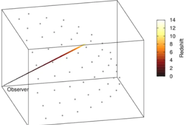
(3) The “Count Matching” Approach for SMGs in the ECDF-S structed and are then used by SAG to generate the galaxy population. The cosmological parameter values assumed are Ωm = 0.28, ΩΛ = 0.72, Ωb = 0.046, H0 = 100 h km s−1 Mpc−1 with h = 0.7 and σ8 = 0.81. These parameters are consistent with WMAP7 data (Jarosik et al. 2011). Below we present a big picture of the SAG model, referring the reader to the papers cited above for a deeper insight on the physical processes included. Hot gas in dark matter halos is isothermally distributed, being drawn from the assumed baryon fraction. It cools according to a cooling rate, forming a galaxy disc that follows an exponential distribution. Stars form at a rate that depends on the amount of cold gas that gives origin to them, besides dark matter halo properties (virial radii and velocities). Cold gas inflows (Dekel et al. 2009) are not included in the current version of the SAG model. Stars can form quiescently as well as in starbursts. Starbursts can be triggered by mergers (both major and minor, defined according to the relative masses of the galaxies involved) and disc instabilities, exhausting all the available cold gas instantaneously and contributing to the bulge growth. A merger of two dark matter halos leads to the merging of the galaxies within them. When a merger occurs, satellite galaxies are accreted by a central one after keeping a circular orbit around it, decaying via dynamical friction. Furthermore, a disc becomes unstable when it is massive enough to be dominated by self-gravity, and therefore sensitive to small external perturbations. Both mergers and disc instabilities, besides cold gas accretion, contribute to the growth of a central black hole. The stellar mass created in each star formation event gives a distinctive number of core-collapse supernovae according to the adopted IMF, which in this model is Salpeter (Salpeter 1955). These supernovae in turn will reheat the cold gas through galactic outflows, transferring it to the hot gas phase. Apart from this kind of feedback, the model considers the heating produced by the active galactic nucleus (AGN) through black hole accretion as responsible of the gas cooling suppression. Star formation events lead to metal pollution in galaxies, yielded via mass losses through stellar winds in stars having low or intermediate mass, as well as supernovae explosions. The chemical enrichment of the gas affects cooling rates and so star formation. The degree of efficiency, as well as the fulfillment of several criteria involved in the different physical processes, are regulated by free parameters. These are tuned in order to reproduce a number of z = 0 observables (see Appendix A, where also some of the galaxy properties predicted by the model and not used as constraints are presented). After assuring this, those parameters remain fixed throughout this work, such that none of the values used is dependent on SMG properties (neither from the model itself nor from observational ones).. 3 CONSTRUCTING LIGHTCONES We use the SAG semi-analytic model within the ΛCDM framework to follow the history of galaxies, obtaining information about them at different epochs which are given by the chosen output redshifts for the model (i.e., the snapshots mentioned in the previous section). We assume that the galaxy sample inside the periodic comoving box of 150 h−1 Mpc a side is statistically representative of the overall galaxy population in the Universe, such that we can build a simulated universe repeating (if necessary) in our simulated catalogs semi-analytic galaxies at different epochs of their evolution. For constructing the simulated universe, the observer is placed at the center of a sphere whose radius extends to the highest redshift c 2014 RAS, MNRAS 000, 1–21. 3. Figure 1. Lightcone construction scheme. Consider the first octant of a sphere filled with semi-analytic galaxies and centered on the observer. A given interval in RA and Dec (sky plane) and redshift z (line of sight) is chosen, collecting all the model galaxies that fall within that region (dots coloured by z). This section of the sphere is mapped taking different orientations (centers indicated by gray points).. where a semi-analytic galaxy exists. The whole spherical volume is populated with galaxies taken from the simulated boxes. Since the redshift separation between two consecutive snapshots is smaller than that corresponding to the side of the box, only one box per epoch is needed in the radial direction. A lightcone consists of all the galaxies that belong to a particular region in the sky and redshift range (see Fig. 1), so the choice of a line of sight and limits in right ascension (RA) and declination (Dec) around it are needed. These are chosen as follows1 . Since our aim is to study the counts in the ECDF-S field, we select the same angular area surveyed by LESS, i.e., ∼ 30′ × 30′ . At the redshifts of interest, this area is smaller than the area subtended by the simulation box, so at a given epoch galaxies appear only once in the area covered by the lightcone. For a given line of sight, the repetition of a model galaxy at various redshifts is limited as much as possible, since the repetition of simulated structure might lead to a wrong interpretation of how model galaxies are spatially distributed once we turn them into a map. In order to test the amount of sources appearing in the lightcone at more than one epoch, we map the first octant of the sphere in the redshift range 0 < z < 5 with 58 lightcones having 0.3 deg2 and orientations with roughly uniform coverage in RA and Dec. Instead of using semi-analytic galaxies, the periodic boxes are filled with a Cartesian grid of dots; they emulate galaxies, so these dots are labeled for keeping control of their frequency of appearance at different epochs. A catalog is then created for each lightcone containing all the “grid galaxies” that fall within it, and a quality factor is computed for evaluating the repetition of structures. This factor is defined as Q=. # points appearing more than once , # points appearing just once. (1). i.e., the ratio between the amount of sources that appear at more than one epoch and the amount of sources that are not repeated. 1 In the following, we do not include any characteristic of the real sky in the simulated celestial sphere, so none of the selected orientations need to be corrected for the presence of the Milky Way, closeness to bright stars, etc..
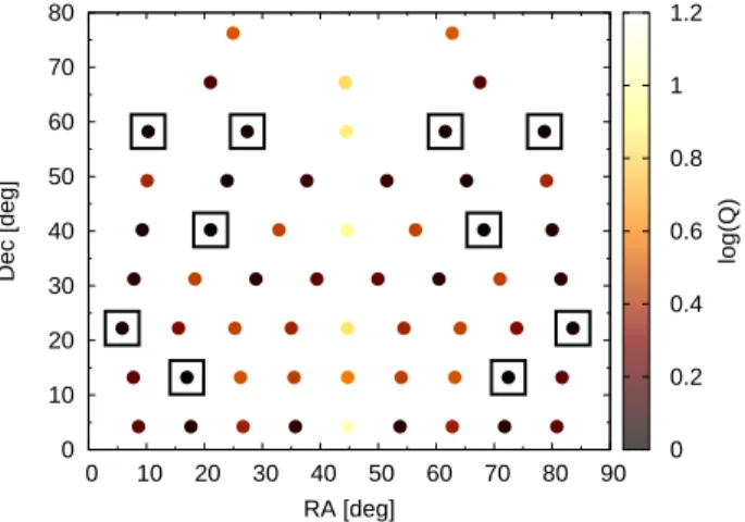
(4) 4. A. M. Muñoz Arancibia et al. 80. Table 1. Quantities used as proxies for the rest-frame submm luminosity.. 1.2. 70. 1 0.8. 50 40. 0.6. 30. log(Q). Dec [deg]. 60. 0.4. 20 0.2. 10 0. Proxy. Definition. Stellar Mass SFR SFR Surface Density sSFR Dust Mass MDA MDD MDS H13. Mstellar Star formation rate SFR/rd2 (for rd > 0) SFR/Mstellar Mdust Mdust /tstellar Mdust × SFR/rd2 (for rd > 0) Mdust × SFR 0.54 × SFR0.43 Mdust. 0 0. 10. 20. 30. 40 50 RA [deg]. 60. 70. 80. 90. Figure 2. Study of the best orientations for the lightcones in RA and Dec, according to the Q quality factor (see text). Orientations indicated in Fig. 1 are filled with dots representing galaxies, drawn from a cubic grid in the range z = 0 to 5, taking angular areas of 0.3 deg2 . For each orientation, Q is computed (colour code gives its logarithm). The n best orientations are such that Q is lowest (black squares). For this paper n = 10 lightcones were selected.. within the lightcone. With this definition, a low repetition of structure is expressed as low Q. We choose the n best orientations as those with the lowest Q. For this paper, n = 10 lightcones were selected (see Fig. 2). The choice of this number of orientations has the aim of testing the effects of cosmic variance over the results. The 58 orientations tested span a range in Q from 1.14 to 12.66, with the ten chosen lightcones in the range Q = 1.14 − 1.24. Through the analysis of galaxy properties presented in this work, we have checked that there are no trends between Q values and the recovered distributions for these ten lightcones. This technique for choosing the best orientations for lightcones was tested only up to z = 5. Since we are interested in galaxy redshift distributions of observed SMGs, which peak at z ∼ 2, this upper limit is adequate for our purposes. Once a lightcone is constructed, the redshifts of galaxies are computed from their coordinates within it. Identifying the particular snapshots of the simulation to which they belong, several galaxy properties given by SAG can be recovered, e.g., stellar masses, SFRs, etc.. 4 THE COUNT MATCHING TECHNIQUE Motivated by abundance matching techniques (e.g., Conroy et al. 2006), we propose a new approach for exploring the properties of SMGs, namely the count matching technique. Here, a given physical galaxy property (or a combination of several ones) is chosen as a proxy for another property whose numerical value is unknown, assuming a monotonic relationship. In our case, the unknowns are the 870 µ m luminosities of a galaxy sample. We use this monotonic relationship to assign a third property, namely, the 870 µ m flux density, to the simulated galaxies in such a way that an observational statistics for the latter is reproduced. The chosen observational statistics are the observed galaxy number counts at this wavelength. This allows to explore several other statistics for simulated galaxies selected using the matched fluxes, like redshifts, masses, luminosities, etc. By comparing them with distributions de-. rived from observations, the quality of the proposed proxies can be analyzed. The selection of properties used in the proxies is motivated by the theoretical understanding of the mechanism that triggers FIR and submm emission in luminous and ultraluminous infrared galaxies (LIRGs and ULIRGs, respectively, Sanders & Mirabel 1996), with the SMGs being thought of as the high-z cousins of these sources. These galaxies emit the bulk of their bolometric emission in the FIR, corresponding to absorbed UV light by dust that is thermally re-radiated at FIR wavelengths; this UV light comes mostly from young stars, with a minor contribution from AGN2 . Within this picture, it makes sense to propose that the bright submm fluxes measured for these sources are correlated in some way with the stellar mass, for instance, in a very simplistic model motivated by the strong correlation of many galaxy properties with stellar mass and the observation of large stellar masses for SMGs (e.g., Michałowski et al. 2010). Or with the dust mass, that partially reprocesses the short wavelength light, or with the star formation rate, as high values give rise to more stars and then more UV emission. Given its low computational cost, the technique offers us the advantage to explore the relationship between several properties (or combinations of them) available from the simulation, and the FIR emission in a galaxy. We are interested in applying this technique when simulating sources in the ECDF-S, given the well studied SMGs detected using the LABOCA bolometer (Weiss et al. 2009) and the recently detected sources using the ALMA interferometer at high submm flux densities (Karim et al. 2013). The steps for this approach are the following: (i) Select a galaxy sample. We take all the galaxies within each lightcone with stellar mass over 108 M⊙ . This lower limit is imposed by the mass resolution of the underlying cosmological simulation; the luminosity functions obtained for our semi-analytic galaxies can be considered complete till that limit (see Ruiz et al. 2014). (ii) Choose a physical galaxy property as a proxy for the 870 µ m rest-frame luminosity, assuming that sources having higher values of the property have higher luminosities. With this we are imposing a monotonic relationship between proxy and luminosity, without placing any restriction about the exact shape of this relation (which can vary depending on the chosen proxy). We test several properties given by SAG, as well as combinations of two or more. The chosen Wang et al. (2013) found a fraction of AGN of 17+16 −6 per cent for ALESS SMGs having a rest-frame 0.5 − 8 keV absorption-corrected luminosity greater than 7.8 × 1042 erg/s. Moreover, Laird et al. (2010) found that in at least ∼ 85 per cent of GOODS-N SMGs the star formation dominates the FIR emission, via the study of their X-ray spectra. 2. c 2014 RAS, MNRAS 000, 1–21.
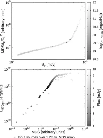
(5) The “Count Matching” Approach for SMGs in the ECDF-S 109. to the observed 870 µ m flux density through. MDS/fk/DL2 [arbitrary units]. 32. 31 30.5 30 29.5. 107. log(L870um [erg/s/Hz]). 31.5. 108. 29. 100. 101. Sν [mJy]. 1032. 28.5 10 9. 7 6 5. 1030. 4. Flux [mJy]. L870um [erg/s/Hz]. 8. 1031. 3. 10. 2. 29. 1011. 1012. 1013. 1014. MDS [arbitrary units]. 1015. 1016. 1. Input sources over 1.2mJy, MDS proxy. Figure 3. The count matching process. Top panel: relation between the 870 µ m flux and the flux-analog quantity y = Proxy/ fk /D2L for the MDS proxy. Bottom panel: recovered relation between rest-frame 870 µ m luminosity and proxy value. For clarity, this is shown only for sources brighter than 1.2 mJy for a given lightcone.. S870 µ m =. properties are: stellar mass (Mstellar ), star formation rate (SFR), cold gas mass (Mcold gas ), disc scale length (rd ), dust mass (Mdust ), stellar age (tstellar ) and cold gas phase metallicity (log(O/H) + 12). The proxies constructed with these properties are defined in Table 1. The H13 proxy corresponds to the eq. 15 of Hayward et al. (2013), 0.54 × SFR0.43 , being the best fit over their simulated galaxi.e. Mdust ies. For the MDA, MDD, MDS and H13 proxies, the dust mass is computed assuming Mdust ∝ Mcold gas × (log(O/H) + 12). This is inspired by the assumption of a dust-to-gas mass ratio proportional to the metallicity,adopted by the radiative transfer code GRASIL (Silva et al. 1998). (iii) For a given property or a combination of properties, let the proxy value, adjusted for cosmological distance, be known as Proxy , fk D2L. (2). and sort the values for all galaxies in increasing order. Here DL is the luminosity distance of each galaxy and fk is a factor giving the k-correction corresponding to its redshift (Hogg et al. 2002) at rest-frame 870 µ m, defined in terms of redshift and monochromatic luminosities (in the Lν formalism) as L870 µ m fk = . (3) (1 + z) L870 µ m/(1+z) Note that the definition of y introduced above turns it into an analog to a flux density (despite its arbitrary units, which vary according to the proxy), since the rest-frame 870 µ m luminosity can be related c 2014 RAS, MNRAS 000, 1–21. L870 µ m . 4π fk D2L. (4). The k-correction is recovered using a template for Arp220 (Blain 1999), which is a typical ULIRG. Additionally, we explore the effect of assuming that the negative k-correction eliminates completely the diminution of the submm flux due to distance; in this approach, the amount of submm flux assigned to each galaxy only depends on the value of the property or combination of properties selected as proxy. (iv) Assign a submm flux to each galaxy according to its value of y, such that sources with higher values will have higher fluxes. This is the key step in the count matching process. Submm fluxes are drawn from a Monte Carlo simulation following the observed cumulative number counts, where we have combined the LABOCA counts at low fluxes (Weiss et al. 2009) and ALMA counts (Karim et al. 2013) over 8 mJy; the choice of ALMA counts only for the bright end is because we want to test whether we are able to recover the LABOCA counts after simulating the observational process (including blending), while avoiding biases in the ALMA counts arising from targeting only bright LESS sources and not other regions in the ECDF-S with signal-to-noise ratios slightly lower than the LESS threshold (Karim et al. 2013) (we tested the effect of switching counts between ALMA and LABOCA data at different fluxes in the range 7.5 − 8.5 mJy, which does not lead to significantly different results). We translate this combination of cumulative counts into differential counts, and use one realization of the Monte Carlo simulation as the random fluxes that follow these counts. The assignment of submm fluxes for galaxies in the lightcone can be summarized as Z ∞ S′ν. y=. 5. n(Sν )dSν =. Z ∞. n(y)dy. (5). Y. where Sν is the flux density at 870 µ m and n(Sν ) is the amount of galaxies having flux densities between Sν and Sν + dSν (and similarly for n(y)). Y and Sν′ stand for particular values of y and Sν . Then Y (Sν′ ) gives the transformation from flux to proxy, which in turn can be used to recover the numerical value of the submm luminosity for each galaxy. To illustrate the procedure, in Fig. 3 top panel we show the relation between the 870 µ m flux, which comes from the Monte Carlo simulation, and the flux-analog quantity y for the MDS proxy, which comes from the model (for clarity, this is only shown for sources over 1.2 mJy for a given lightcone). Once the 870 µ m flux is assigned to a given galaxy, the SED template can be used to recover the numerical value of its rest-frame 870 µ m luminosity. The shape of the monotonic relation between this luminosity and the proxy value for MDS is shown in the bottom panel; the trend is robust, despite some outliers having combinations of extreme proxy and redshift values. Proxies proposed in this work then have simple, one-to-one dependences with rest-frame 870 µ m luminosity, for a stellar mass limited sample of model galaxies. No additional selections are included at this stage, except for sources where a proxy has an undefined value (e.g., removing galaxies without disc in SFR surface density and MDD proxies). Definitely, these proxies can be refined selecting only a subset of the stellar mass limited sample, for instance removing passive galaxies because of their low SFR; we leave these improvements for a future work..
(6) 6. A. M. Muñoz Arancibia et al. 16. 14. Sν,deboosted [mJy]. 12. 10. 8. 6. 4. 2. 2. 4. 6. 8. 10. 12. 14. 16. Sν,extracted [mJy] 103. The advantage of using this simple recipe instead of a full radiative transfer is the considerably lower computational cost, when applied to big samples of galaxies. However, it also has limitations. In the abundance matching formalism, the halo mass function must be correctly predicted by the N-body simulation, as well as the stellar mass function should be well derived from the observations. In our approach, we are assuming that the bright-end ALMA and faint-end LABOCA counts are correct, an observable that does not provide redshift information. Because submm luminosities are difficult to model directly, we choose a proxy for the rest-frame submm luminosity for each model galaxy, and use its redshift and an appropriate SED template to predict its submm flux analog. We then perform an abundance-type matching in the space of observed vs predicted submm fluxes following Eq. 5. This determines the redshift distribution of the brightest sources (i.e. SMGs) as a function of flux, which in turn influences their clustering and therefore the amount of blending that occurs before bright-end LABOCA counts are measured.. 5 SIMULATING THE OBSERVATIONAL PROCESS We turn the catalogs of galaxy positions and fluxes given by the different proxies into submm maps that include a modeling of the observational process. First, simulated sources are injected in a noise map having a spatial resolution of 19.5′′ (as the LABOCA beamwidth). The resulting map is beamsmoothed using a 90′′ Gaussian kernel, for removing low spatial frequency structures as is commonly done for observational data (e.g., Weiss et al. 2009). The latter map is then substracted from the former, and the result is convolved with a 19.5′′ Gaussian kernel, giving rise to a map resolution of 27.6′′ . The beamsmoothing process produces a decrease in the source fluxes by ∼ 8.6 per cent, which are hence rescaled.. 102. N(>Sν) [deg−2]. Figure 4. Example of a simulated map, corresponding to a given lightcone in the MDS proxy. The black square encloses the region where simulated sources are injected (∼ 30′ × 30′ ). Grayscale gives submm flux per pixel. The map resolution is 6′′ /pix.. 101 Weiss et al. (2009) counts This work, using extracted fluxes This work, using deboosted fluxes. 100. 2. 3. 4. 5. 6. 7. 8. 9 10 11 12131415. Sν [mJy] Figure 5. Source extraction and flux deboosting methods used in this work, applied to the actual LESS map (Weiss et al. 2009). Top panel: comparison between extracted and deboosted fluxes for our detected sources. Bottom panel: cumulative number counts recovered in each case, compared to actual data for this field (Weiss et al. 2009).. One map is constructed for each orientation and proxy. Injected sources span a region of ∼ 30′ × 30′ . They are taken from the simulated lightcones, being the N brightest sources of each catalog. We choose N = 5 × 10³ , as it gives source fluxes well below the values reported by observations, while the computing time is reasonable (we checked that a change in one order of magnitude in N does not have a significant effect on the statistics recovered from the maps). An example of these simulated maps is given in Fig. 4, indicating the region where model sources are injected as a black square. We perform a source extraction as done for maps obtained through observations. With this we study the effects of the observational process on the recovered counts, as well as the galaxy properties derived from the counterparts of detected sources for each proxy. Sources are extracted using SE XTRACTOR (Bertin & Arnouts 1996), for a limit in S/N of 3.8. This cut is chosen following Weiss et al. (2009), according to the expected number of false dec 2014 RAS, MNRAS 000, 1–21.
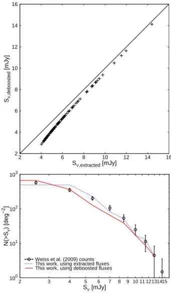
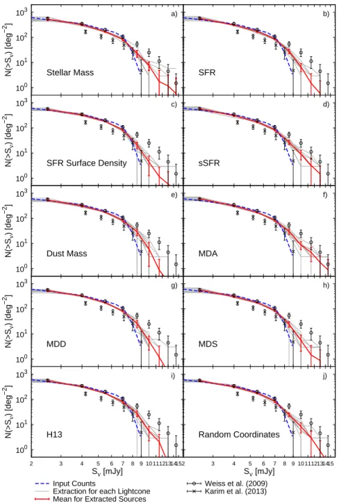
(7) The “Count Matching” Approach for SMGs in the ECDF-S tections. The source extraction comprises two iterations, where in the second one the sources detected in the first iteration are removed from the map and the noise level is recalculated. We consider even sources extracted outside the limits given by the injected sources. As our resulting source catalog is limited by S/N, we need to correct the extracted fluxes for boosting effects: the systematic enhancement on the measured fluxes coming from noise introduces a bias in the number of sources exceeding the chosen limit (Scott et al. 2008). For simulated maps, the deboosting correction is found comparing the extracted flux of a given source with the flux of its brightest counterpart in the input catalog (see Section 6.1) and then using the fitting function Sν ,deboosted = (Sν ,extracted + A)1/2 , with A the free parameter. This function is chosen such that it has a cutoff at fluxes near the S/N limit, and tends to the equality at high fluxes. Taking these deboosted fluxes, cumulative submm number counts are obtained for each simulated map, including a proper correction for completeness taken from Weiss et al. (2009). In order to validate these methods of source extraction and flux deboosting, we apply them to the actual LESS field (Weiss et al. 2009): first, we extract sources from the actual LESS map down to S/N = 3.8 with SE XTRACTOR, and secondly we apply the flux deboosting correction to the extracted sources. Since in this case the map comes from real observations, we do not have an input catalog for it, so the A parameter is found computing the median value among all the simulated maps. The resulting deboosted fluxes and counts are shown in Fig. 5. Compared to Weiss et al. (2009) data, we recover a lower amount of sources in the flux range ∼ 4 − 8 mJy by a factor ∼ 1.5. However, this may come from their different deboosting flux technique, which makes use of a P(D) analysis. We have tried different parameters for SE XTRAC TOR . In a first extraction with conservative parameters (DETECT MINAREA=5 plus defaults) and only one iteration, we obtained ∼ 20 per cent less sources than reported by Weiss et al. (2009). Trying with a grid of parameters in DETECT MINAREA, and also modifying the parameters related to the deblending of sources (DEBLEND NTHRESH and DEBLEND MINCONT), we increased the matching with the original catalog. Finally, after extracting the sources from the first iteration, we re-run SE XTRACTOR on the residual map. This procedure assures us a good agreement with the catalog from Weiss et al. (2009), thus minimizing differences in the final counts arising from different detection methods.. 6 RESULTS AND DISCUSSION We are interested in those proxies where the simulated sources that follow the observed LABOCA plus bright-end ALMA counts, after going through the observational process, give 1) counts comparable to LABOCA data, 2) redshift distributions consistent with observational values, 3) other properties in agreement with observations (including clustering, stellar mass, host halo mass, etc). For the last two requirements, we compare model distributions with different surveys from the literature. Note that it is possible that the properties are affected by the environment of ECDF-S, as this field appears to be underdense when compared to other deep fields probed with submm wavebands (see Weiss et al. 2009 discussion, but also Chen et al. 2013, who find no difference with other fields but for a smaller area). However, we find that there are only minor changes in the proxy vs luminosity at 870 µ m relation (see Fig. 3) between lightcones of c 2014 RAS, MNRAS 000, 1–21. 7. different density. In particular, this relation changes only by ∼ 10 per cent between the different lightcones for the MDS proxy.. 6.1 Number Counts Fig. 6 shows the cumulative submm number counts obtained for the different proxies, compared to the input number counts (i.e., before passing through the observational process) and to those extracted from LABOCA and ALMA observations. Compared to the observed counts, sources extracted from the simulated maps give counts closer to LABOCA data. In order to quantify the goodness of each proxy at this step, we compare their χ 2 values given by. χ2 = ∑ Sν. [(dN/dS)LABOCA − (dN/dS)]2 [δ (dN/dS)LABOCA ]2 + [δ (dN/dS)]2. ,. (6). where (dN/dS)LABOCA corresponds to the observed LABOCA differential counts at a given flux density, (dN/dS) gives our mean differential counts over the ten lightcones, and δ (dN/dS), δ (dN/dS) values are the reported uncertainties in LABOCA counts and scatter in our simulated counts, respectively. Since sources injected in the maps follow the combined bright-ALMA plus faint-LABOCA counts by construction, this χ 2 definition allow us to quantify the influence coming from a) the observational process (blending, noise, etc) and b) clustering given by the model (as different proxies give different spatial distribution for bright sources). The reduced χ 2 is presented for all proxies in Table 2, second column. There, as well as in Fig. 6, we also show the results for the case where the spatial distribution of input sources along each of the ten maps is random, i.e., does not come from any proxy and so no clustering is provided (note that the number of sources injected in each map is the same as used for the proxies, as well as their submm flux distribution). All proxies are quite similar, so this criterion is not enough to choose a proxy as the best. A further analysis of the predicted distribution of other galaxy properties may discriminate better between proxies. Even the counts obtained for input sources with randomized positions in the simulated map are consistent with those where the count matching process was applied (which include realistic galaxy clustering provided by the semi-analytic model). This finding indicates that the clustering has a minor influence when determining the cumulative submm number counts. For recovering the properties of model galaxies, we perform a cross-match between all the extracted sources and the input galaxies having submm fluxes down to 1.2 mJy (hereafter the input catalog). A search radius of 13.8′′ is used, corresponding to the beam radius after the map processing (see Section 5). When more than one input galaxy falls within the search radius around a given extracted source, we refer to it as a multiple source composed by blended galaxies; otherwise, we call it a single source. Fig. 7 illustrates this with a small region within the map shown in Fig. 4. Note that among the extracted sources, besides singles and multiples there can be also sources that do not have a counterpart in the input catalog. Although most of these non-matched sources have S/N ratios around the chosen limit for extraction and can be considered as spurious sources whose flux is boosted by the map noise, some of them have S/N over 5. A fraction of ∼ 22−25 per cent of the extracted sources do not have counterparts (see Table 2, third column); in the following, we remove these sources from our analyses. The fraction of multiple sources across the proxies, in the flux range given by the recovered.
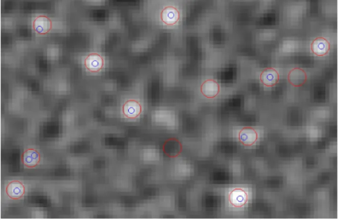
(8) 8. A. M. Muñoz Arancibia et al.. N(>Sν) [deg−2]. 103. a). 102 101. Stellar Mass 10. SFR. 0. 103. N(>Sν) [deg−2]. b). c). d). 102 101. SFR Surface Density. sSFR. 100. N(>Sν) [deg−2]. 103. e). 102 101. Dust Mass 10. MDA. 0. N(>Sν) [deg−2]. 103. g). h). 102 101. MDD 10. MDS. 0. 103. N(>Sν) [deg−2]. f). i). j). 102 101. H13 10. Random Coordinates. 0 2. 3. 4. 5. 6. 7. 8 9 10 11121314152. Sν [mJy] Input Counts Extraction for each Lightcone Mean for Extracted Sources. 3. 4. 5. 6. 7. 8 9 10 1112131415. Sν [mJy] Weiss et al. (2009) Karim et al. (2013). Figure 6. Cumulative number counts at 870 µ m obtained for the different proxies: a) stellar mass, b) SFR, c) SFR surface density, d) specific SFR (sSFR), e) dust mass, f) dust mass divided by stellar age (MDA), g) dust mass times SFR divided by the square of the disc scale length (MDD), h) dust mass times SFR (MDS), and i) eq. 15 of Hayward et al. (2013) (H13). Blue thick dashed lines give the input counts for each proxy, using all the input galaxy fluxes given by the count matching. Gray thin solid lines correspond to the counts recovered for the ten lightcones after passing through the observational process, i.e., obtained from sources extracted from the simulated maps. Red thick solid lines connect mean values for simulated sources at each flux level, with standard deviations as errorbars. As a comparison, observational data are shown from LABOCA (Weiss et al. 2009) and ALMA studies (Karim et al. 2013). Additionally, counts obtained for input sources with randomized positions in the simulated map are given in panel j). In all panels, there are lines of sight giving counts consistent with those derived from LABOCA observations.. counts, goes from ∼ 9 to ∼ 14 per cent (see Table 2, fourth column). We have checked that the coordinates of counterparts do not follow a preferential direction in the map when compared to the coordinates of extracted sources.. 6.2 Recovered Redshift Distributions for Detected Sources and k-correction Effects. As shown above, all the proposed proxies (even taking random positions for galaxies in the sky) can successfully reproduce the observed LABOCA counts. We then explore other predicted properc 2014 RAS, MNRAS 000, 1–21.
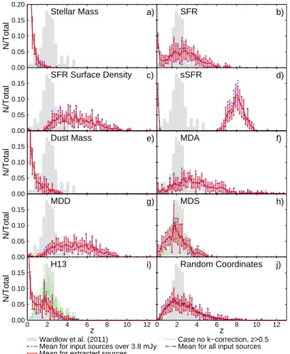
(9) The “Count Matching” Approach for SMGs in the ECDF-S. 9. Table 2. Properties from the counts derived for each proxy, using sources extracted from the simulated maps (extraction down to the 3.8σ detection level). Fractions are mean values over the ten lightcones, reporting also standard deviations. Proxy. χ 2 /dof a. Mean fraction of non-matches b. Mean fraction of multiples c. Stellar Mass SFR SFR Surface Density sSFR Dust Mass MDA MDD MDS H13 Random Coordinates. 3.598 3.120 3.689 3.617 3.536 3.400 3.642 3.558 3.599 3.470. 0.223 ± 0.027 0.250 ± 0.032 0.232 ± 0.029 0.237 ± 0.026 0.243 ± 0.028 0.228 ± 0.021 0.232 ± 0.029 0.244 ± 0.025 0.245 ± 0.041 0.248 ± 0.021. 0.113 ± 0.044 0.105 ± 0.028 0.090 ± 0.033 0.123 ± 0.028 0.091 ± 0.021 0.141 ± 0.034 0.102 ± 0.033 0.096 ± 0.028 0.089 ± 0.034 0.093 ± 0.027. a Reduced χ 2 for each proxy, with χ 2 calculated according to Eq. 6 and dof the degrees of freedom (i.e. number of flux bins). b Mean fraction of sources without having a counterpart in the input catalog (over all the extracted sources). c Mean fraction of sources having more than one counterpart in the input catalog (over the extracted sources that have at least one counterpart).. Figure 7. Small section of the simulated map shown in Fig. 4, illustrating the cross-match between extracted and input sources. Sources extracted from the map lie in the centers of the red big circles, which have a radius of 13.8′′ ; this is the search radius used for finding the counterparts of these sources in the input catalog down to 1.2 mJy, which are shown as blue small circles. They allow us to explore the predicted properties for extracted sources in each lightcone and proxy.. ties of bright model galaxies, to find out which (if any) proxies for submm luminosity are plausible. The properties of extracted sources are recovered assigning to them the galaxy properties of their counterpart(s) in the input catalog. Including in our analysis the properties of all the input sources within the search radius down to 1.2 mJy allows us to compare the distribution of recovered properties for each proxy with statistics derived from observations in the literature, even from follow-ups of single-dish detected SMGs with interferometry. If we restrict the comparison to single-dish detected SMGs, and so assign to a extracted multiple source the properties of the brightest model galaxy within the search radius, there are no significant differences in the recovered distributions compared to the inclusion of all counterparts. This shows that the observational process of source extraction does not impose systematic biases in this respect. In addition, we can compare the observations in the literature with the distributions obtained for input sources brighter than 3.8 mJy, i.e., the c 2014 RAS, MNRAS 000, 1–21. properties of the brightest model galaxies in submm before going through the observational process. Fig. 8 shows the mean redshift distributions for the extracted sources in each proxy. For all proxies, there is no significant difference between them and the distributions for the input brightest sources. The proxy that gives the closest match with the observed distribution (i.e., Wardlow et al. 2011 for the ECDF-S) is MDS, giving mean values around z = 2. Although the SFR proxy gives a distribution with similar shape to the observational one, it has the problem of including a significant fraction of very low-z sources. Hence, even though the MDS proxy prediction is much broader compared to the observed distribution, it provides an acceptable agreement for such a simple model where the rest-frame 870 µ m luminosity is assumed to be related to galaxy properties in a direct dependence (see Fig. 3), suggesting that both dust mass and SFR might play an important role in the process of FIR emission. This dependence can surely be improved. For the brightest sources in the submm, however, redshift distributions also depend on the k-correction factor assumed for the model galaxies, as it affects the assignment of submm fluxes to each galaxy in the sample and thus the flux of sources detected in the simulated maps; similarly, the distributions may change if very low-z sources are excluded in the count matching process. Assuming that the negative k-correction eliminates completely the dilution due to distance, the amount of submm flux assigned to each galaxy only depends on the value of the property selected as proxy; we call this case “no k-correction”, and explore it particularly for the MDS and H13 proxies. The predicted distributions are shown as green histograms in panels h) and i) of Fig. 8 respectively, for comparison with the fiducial case. As it is shown, H13 becomes a good proxy only if model sources having z < 0.5 are excluded in the count matching process. In this case, there are no significant modifications to the shape of the distribution when applying the k-correction to model spectra. The dependence of the submm flux density with dust mass and SFR was addressed in detail by Hayward et al. (2011), using the results of hydrodynamical simulations of isolated disc and merging galaxies connected to a dust radiative transfer code. Hayward et al. (2011) results motivated the fitting function used by Hayward et al. (2013) in the assignment of submm fluxes. They found that this relation is accurate to within 0.3 dex in the redshift range ∼ 1 − 6,.
(10) 10. A. M. Muñoz Arancibia et al.. N/Total. 0.20. Stellar Mass. a). SFR. b). SFR Surface Density. c). sSFR. d). Dust Mass. e). MDA. f). MDD. g). MDS. h). H13. i). Random Coordinates. j). 0.15 0.10 0.05. N/Total. 0.00 0.15 0.10 0.05. N/Total. 0.00 0.15 0.10 0.05. N/Total. 0.00 0.15 0.10 0.05. N/Total. 0.00 0.15 0.10 0.05 0.00. 0. 2. 4. 6. z. 8. 10. 12 0. Wardlow et al. (2011) Mean for input sources over 3.8 mJy Mean for extracted sources. 2. 4. 6. z. 8. 10. 12. Case no k−correction, z>0.5 Mean for all input sources. Figure 8. Mean redshift distributions over the ten lightcones obtained for the different proxies, taking all the sources extracted from simulated maps having counterparts in the catalog of input sources down to 1.2 mJy, considering all the input sources that lie within a search radius of 13.8′′ (red thick solid lines). This is compared to the mean histogram obtained taking all the input sources brighter than 3.8 mJy (blue thin dashed lines). For each proxy the distribution of photometric redshifts obtained by Wardlow et al. (2011) for 78 LESS sources is overplotted (gray histograms). The submm flux for each galaxy in the input catalogs, which give origin to the simulated maps, is obtained according to Eq. 5 (see also Eq. 2), where the k-correction factor is given by an Arp220 template spectrum. The MDS proxy is the only one that is in good qualitative agreement with the observed distribution for the ECDF-S. The H13 proxy only gives a good agreement when model sources having z < 0.5 are excluded in the count matching process (green thick dotted lines); in this case, k-correcting the spectra does not introduce a significant change in the distribution, and MDS remains as a good proxy. Additionally, the last panel shows the distribution recovered when a random assignment of submm luminosities is done for model sources, injected in a map following a random spatial distribution. In this panel we also include the distribution for the whole galaxy population in the simulated lightcones (black thin dot-dashed line).. but severely underpredicts the galaxy fluxes for z . 0.5. Our results are in line with those findings, as the H13 proxy reproduces the observed redshift distribution only when discarding low-redshift sources during the flux assignment. Over z > 0.5, this proxy works applying or not the k-correction factor. It is remarkable that the MDS proxy gives a good agreement with observations even when sources at z < 0.5 are excluded in the count matching process, and independent of the assumption for the shape of the galaxy spectrum. Besides the proposed proxies, we explore the redshift distribution obtained when a random assignment of submm luminosities is done for model sources, which are injected in the simulated map with a random spatial distribution. As is shown in panel j) of Fig. 8, the recovered distribution is wider than the observed for SMGs and reaches its maximum around z = 2, resembling the statistics for the whole galaxy population in the simulated lightcones. We apply some robustness tests to our technique. First, we test the effects of adding scatter to the proxy, in light of the findings by Moster et al. (2010) and Behroozi et al. (2010) about how scatter. can bias the results of the abundance matching. We explore this using a Gaussian distribution centered in the value given by the model and taking a standard deviation of 30 per cent (this choice is close to typical errors in galaxy properties derived from observations, as stellar mass or SFR). After this, the trend between proxy and restframe 870 µ m luminosity is still robust. The recovered redshift distributions are consistent with the ones obtained without considering the scatter, with their medians varying only 0.15 units at most (except for the sSFR proxy, where the median redshift decreases by 0.9 units). In addition, we test the effects that come from using models that give poorer fits to the observed galaxy population. We achieve this modifying two key features in SAG: a) excluding AGNs in the whole model, and b) using the De Lucia et al. (2004) prescription for star formation (fiducial is Croton et al. 2006, which unlike the former involves a cold gas mass density threshold below which there is no star formation). Both tests were done keeping the same model parameters as in the fiducial case. Excluding AGNs changes dramatically the SMG redshift disc 2014 RAS, MNRAS 000, 1–21.
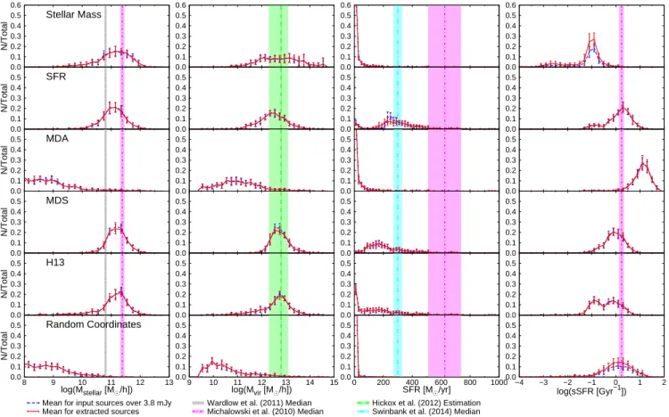
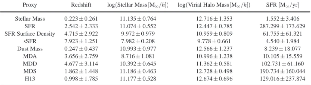
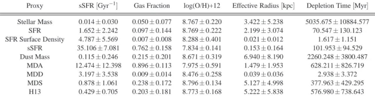
(11) N/Total. N/Total. N/Total. N/Total. N/Total. N/Total. The “Count Matching” Approach for SMGs in the ECDF-S 0.6 0.5 0.4 0.3 0.2 0.1 0.0 0.5 0.4 0.3 0.2 0.1 0.0 0.5 0.4 0.3 0.2 0.1 0.0 0.5 0.4 0.3 0.2 0.1 0.0 0.5 0.4 0.3 0.2 0.1 0.0 0.5 0.4 0.3 0.2 0.1 0.0. Stellar Mass. SFR. MDA. MDS. H13. Random Coordinates. 8. 9. 10. 11. log(Mstellar [M⊙/h]). 12. 13. Mean for input sources over 3.8 mJy Mean for extracted sources. 0.6 0.5 0.4 0.3 0.2 0.1 0.0 0.5 0.4 0.3 0.2 0.1 0.0 0.5 0.4 0.3 0.2 0.1 0.0 0.5 0.4 0.3 0.2 0.1 0.0 0.5 0.4 0.3 0.2 0.1 0.0 0.5 0.4 0.3 0.2 0.1 0.0. 9. 10. 11. 12. 13. log(Mvir [M⊙/h]). 14. Wardlow et al. (2011) Median Michalowski et al. (2010) Median. 15. 0.6 0.5 0.4 0.3 0.2 0.1 0.0 0.5 0.4 0.3 0.2 0.1 0.0 0.5 0.4 0.3 0.2 0.1 0.0 0.5 0.4 0.3 0.2 0.1 0.0 0.5 0.4 0.3 0.2 0.1 0.0 0.5 0.4 0.3 0.2 0.1 0.0. 0. 200. 400. 600. SFR [M⊙/yr]. 800. 0.6 0.5 0.4 0.3 0.2 0.1 0.0 0.5 0.4 0.3 0.2 0.1 0.0 0.5 0.4 0.3 0.2 0.1 0.0 0.5 0.4 0.3 0.2 0.1 0.0 0.5 0.4 0.3 0.2 0.1 0.0 0.5 0.4 0.3 0.2 0.1 0.0 1000 −4. −3. −2. −1. 0. −1. 11. 1. 2. log(sSFR [Gyr ]). Hickox et al. (2012) Estimation Swinbank et al. (2014) Median. Figure 9. Mean distributions over the ten lightcones of several properties obtained for five selected proxies: stellar mass, SFR, dust mass divided by stellar age (MDA), dust mass times SFR (MDS), and eq. 15 of Hayward et al. (2013) (H13). Sources extracted from simulated maps having counterparts in the catalog of input sources down to 1.2 mJy are taken, considering all the input sources that lie within a search radius of 13.8′′ (red solid lines). Properties are compared to the mean histograms obtained taking all the input sources brighter than 3.8 mJy (blue dashed lines). Standard deviations for model distributions are shown as errorbars. In columns from left to right, the predicted properties are: stellar mass, compared to the median values obtained by Wardlow et al. (2011) and Michałowski et al. (2010), in vertical gray dotted and magenta dot-dashed lines respectively; virial halo mass, compared to the Hickox et al. (2012) estimation, as a vertical green long-dashed-dotted line; SFR, compared to the Michałowski et al. (2010) median value as vertical magenta dot-dashed line and to the Swinbank et al. (2014) median value as a vertical cyan dot-dot-dashed line; and specific SFR, compared to Michałowski et al. (2010) median value, again in a vertical magenta dot-dashed line. Standard errors for observational values are presented as coloured shaded regions. Bottom panels show the distributions recovered when a random assignment of submm luminosities is done for model sources, injected in a map following a random spatial distribution.. tribution for the MDS proxy, which now peaks at z = 0.3. For the stellar mass, dust mass and H13 proxies it gives no sources over z = 1, while for the SFR proxy it gives ∼ 3 times more low-z sources in proportion. For this model, none of our proposed proxies gives an acceptable redshift distribution when compared to observational data. The model with the alternative prescription for star formation introduces changes in the SMG redshift distributions for some of the proxies. For the MDS and H13 proxies it gives 2 and 1.6 times more low-z sources in proportion, respectively. For the dust mass proxy it gives 1.5 times more z = 0 sources and essentially zero sources over z = 1. For the SFR surface density proxy it gives no sources below z = 3, while for the MDD proxy there are no SMGs below z = 4. Finally, we tested the effects on the recovered distributions of using the median SED for observed SMGs found by Michałowski et al. (2010) to compute k-corrections, finding no significant differences with respect to the fiducial model except for the sSFR proxy, where the median redshift decreases by 2 units. For the H13 proxy, an extra peak emerges in the predicted redshift distribution at z = 0.8. We also tried Magdis et al. (2012) SED templates as c 2014 RAS, MNRAS 000, 1–21. they allowed Béthermin et al. (2012) to reproduce the counts from the mid-IR to the mm domain using an empirical model. Using these templates we find no significant differences with respect to the fiducial model. For instance, in the SFR, MDS and H13 proxies the median redshift moves to a lower value by ∼ 0.5 units. To sum up, the changes from modifications to the model produce small changes in the results as long as the z = 0 model galaxies are consistent with observations. 6.3 Prediction of Physical Properties of SMGs Our analysis of the submm extracted sources is also extensible to other galaxy properties given by the semi-analytic model. Figs. 9 and 10 show some of the distributions predicted when taking kcorrected galaxies at z > 0 in the count matching process: stellar mass, halo mass, SFR, sSFR, gas fraction, cold gas phase metallicity, effective radius and depletion time. Note that the intrinsic values of these properties are not affected by the count matching, since they are computed entirely by the SAG model. Keeping the values of these properties without modifications, assures that the final SAG galaxy population remains unaffected by the count matching.
(12) N/Total. N/Total. N/Total. N/Total. N/Total. N/Total. 12. A. M. Muñoz Arancibia et al.. 0.6 0.5 0.4 0.3 0.2 0.1 0.0 0.5 0.4 0.3 0.2 0.1 0.0 0.5 0.4 0.3 0.2 0.1 0.0 0.5 0.4 0.3 0.2 0.1 0.0 0.5 0.4 0.3 0.2 0.1 0.0 0.5 0.4 0.3 0.2 0.1 0.0 0.0. Stellar Mass. SFR. MDA. MDS. H13. Random Coordinates. 0.2. 0.4. 0.6. 0.8. 1.0. 0.6 0.5 0.4 0.3 0.2 0.1 0.0 0.5 0.4 0.3 0.2 0.1 0.0 0.5 0.4 0.3 0.2 0.1 0.0 0.5 0.4 0.3 0.2 0.1 0.0 0.5 0.4 0.3 0.2 0.1 0.0 0.5 0.4 0.3 0.2 0.1 0.0. 6. 7. Gas Fraction Mean for input sources over 3.8 mJy Mean for extracted sources. 8. 9. 10. 11. 0.6 0.5 0.4 0.3 0.2 0.1 0.0 0.5 0.4 0.3 0.2 0.1 0.0 0.5 0.4 0.3 0.2 0.1 0.0 0.5 0.4 0.3 0.2 0.1 0.0 0.5 0.4 0.3 0.2 0.1 0.0 0.5 0.4 0.3 0.2 0.1 0.0. 0. log(O/H)+12. 5. 10. 15. 20. 25. Effective Radius [kpc]. Tacconi et al. (2006) Median Swinbank et al. (2004) Average. Targett et al. (2013) Average Rujopakarn et al. (2011) Median. 0.6 0.5 0.4 0.3 0.2 0.1 0.0 0.5 0.4 0.3 0.2 0.1 0.0 0.5 0.4 0.3 0.2 0.1 0.0 0.5 0.4 0.3 0.2 0.1 0.0 0.5 0.4 0.3 0.2 0.1 0.0 0.5 0.4 0.3 0.2 0.1 0.0. −2. 0. 2. 4. 6. log(Depletion Time [Myr]) Tacconi et al. (2008) Timescale. Figure 10. Mean distributions over the ten lightcones of several properties obtained for five selected proxies: stellar mass, SFR, dust mass divided by stellar age (MDA), dust mass times SFR (MDS), and eq. 15 of Hayward et al. (2013) (H13), with red solid and blue dashed lines as in Fig. 9. In columns from left to right, the predicted properties are: gas fraction, defined as cold gas mass over the sum between cold gas and stellar mass, compared to the median value found by Tacconi et al. (2006) as a vertical gray dot-dashed line; cold gas phase metallicity in terms of oxygen and hydrogen abundances, compared to the average value found by Swinbank et al. (2004) as a vertical green dot-dot-dashed line; effective radius, computed considering the contribution of both bulge and disc, compared with values found by Targett et al. (2013) and Rujopakarn et al. (2011) in vertical cyan long-dashed-dotted and orange dotted lines respectively; and depletion time, defined as the ratio between the cold gas mass and SFR, compared to the gas exhaustion timescale found by Tacconi et al. (2008) as a vertical magenta double-dotted line. Bottom panels show the distributions recovered when a random assignment of submm luminosities is done for model sources, injected in a map following a random spatial distribution.. Table 3. Properties of sources extracted from the simulated maps. Uncertainties for each proxy are standard deviations of the median, considering all sources belonging to the 10 lightcones altogether. Proxy. Redshift. log(Stellar Mass [M⊙ /h]). log(Virial Halo Mass [M⊙ /h]). SFR [M⊙ /yr]. Stellar Mass SFR SFR Surface Density sSFR Dust Mass MDA MDD MDS H13. 0.223 ± 0.261 2.542 ± 2.333 4.715 ± 2.922 7.923 ± 1.251 0.247 ± 0.437 3.656 ± 2.759 4.677 ± 3.114 1.862 ± 1.448 0.998 ± 1.785. 11.135 ± 0.764 11.074 ± 0.552 9.972 ± 0.979 7.982 ± 0.208 10.993 ± 0.977 8.716 ± 1.081 10.392 ± 0.645 11.186 ± 0.463 11.177 ± 0.528. 12.716 ± 1.353 12.447 ± 0.785 10.959 ± 0.809 9.778 ± 0.661 12.566 ± 1.237 10.996 ± 1.238 11.362 ± 0.581 12.728 ± 0.498 12.674 ± 0.696. 1.552 ± 3.406 287.299 ± 173.629 61.755 ± 61.321 4.540 ± 1.984 8.239 ± 18.077 10.105 ± 15.559 102.731 ± 61.160 190.734 ± 160.044 129.016 ± 237.874. technique. What may vary across the proposed proxies are the distributions of these properties for bright SMGs, since model sources having assigned the highest 870 µ m flux densities for one proxy could have, for instance, intrinsically lower SFRs when compared to model bright sources selected using another proxy.. All the properties listed above can be compared with observa-. tions3 . For brevity, this is presented only for five of the proxies; we select the proxies giving the best agreement with the observed red-. 3 When comparing results for the proxies with observational properties that depend on assumed evolutionary synthesis models, we do not make any rescaling for IMFs different from the one assumed in this work (Salpeter IMF).. c 2014 RAS, MNRAS 000, 1–21.
(13) The “Count Matching” Approach for SMGs in the ECDF-S. 13. Table 4. Properties of sources extracted from the simulated maps (cont.). Proxy. sSFR [Gyr−1 ]. Gas Fraction. log(O/H)+12. Effective Radius [kpc]. Depletion Time [Myr]. Stellar Mass SFR SFR Surface Density sSFR Dust Mass MDA MDD MDS H13. 0.014 ± 0.030 1.652 ± 2.242 4.787 ± 5.569 35.106 ± 7.081 0.115 ± 0.246 12.474 ± 12.398 3.197 ± 3.538 0.878 ± 1.061 0.429 ± 0.705. 0.050 ± 0.077 0.097 ± 0.144 0.007 ± 0.008 0.762 ± 0.158 0.215 ± 0.201 0.896 ± 0.113 0.009 ± 0.014 0.238 ± 0.172 0.203 ± 0.181. 8.767 ± 0.220 8.769 ± 0.222 8.288 ± 0.401 7.834 ± 0.141 8.671 ± 0.319 7.975 ± 0.591 8.476 ± 0.258 8.796 ± 0.134 8.773 ± 0.168. 3.422 ± 5.238 2.199 ± 3.074 0.021 ± 0.012 0.153 ± 0.164 6.940 ± 8.190 1.479 ± 1.953 0.039 ± 0.036 5.127 ± 4.998 5.222 ± 5.838. 5035.675 ± 10884.577 70.547 ± 130.123 1.617 ± 1.151 101.953 ± 94.529 2260.248 ± 3800.487 628.211 ± 826.719 2.938 ± 3.372 377.963 ± 429.295 576.980 ± 738.643. shift distribution shown in Fig. 8, as well as some of the proxies that do not. This is done in order to check if the former ones predict, in a consistent way, other galaxy properties when compared to observations. Median values for these properties are shown in Tables 3 and 4. The Arp220 template is used for k-correcting the galaxy spectra. Again, there is no significant difference between the recovered distributions and those for the input brightest sources. We compare the distribution of stellar masses with the median values derived by Wardlow et al. (2011) and Michałowski et al. (2010), who consider single-dish detected sources mapping the submm continuum; the former analyze 78 detected counterparts to 72 SMGs in the ECDF-S, while the latter consider 76 SMGs from the Chapman et al. (2005) sample. Except for the MDA proxy, all of them give reasonable distributions compared to SMG observations; note that the standard errors reported for observational quantities do not take into account the individual uncertainties in their determination. However, moving to the predicted virial halo masses, we find that only MDS and H13 proxies are able to reproduce the value estimated by Hickox et al. (2012) for SMGs in the ECDF-S field. Our model underpredicts the SFRs by a factor of ∼ 3 when compared to observed values for SMGs by Michałowski et al. (2010), being more consistent with SFRs measured for high-z starforming galaxies (SFGs) by Tacconi et al. (2010), which have mean values of 95 and 135 M⊙ /yr at z = 1.2 and 2.3 respectively (note that this is not a sample of SMGs). Deblending FIR observations for the ALESS SMG positions with Herschel, Swinbank et al. (2014) find a median SFR ∼ 2 times lower than the one derived for singledish selected SMGs, although their sample includes 870 µ m fluxes down to 2 mJy (including only sources brighter than 4.2 mJy gives an SFR of 530 ± 60 M⊙ /yr). Regarding the sSFR distribution, the stellar mass proxy gives considerably lower values compared to the median value found by Michałowski et al. (2010), the MDA proxy considerably higher values, and the H13 proxy a bimodal distribution; the remaining proxies give a reasonable prediction. Reproducing the observed SFR distribution for SMGs is an outstanding challenge for semi-analytic models. Some aspects in SAG regarding the modeling of the star formation (e.g. the complete removal of hot gas when galaxies become satellites, or not including cold gas inflows) might be leading to lower predicted SFRs not only for SMGs, but also for the whole galaxy population across redshift (see the discussion about Fig. A1 in Appendix A). This translates in globally underpredicting galaxy SFRs at the redshifts where SMGs lie. It affects the predicted distributions for SMGs given by all our proposed proxies, recalling that the intrinsic SFR of each galaxy is not affected by the count matching process. However, for each model SMG we can explore the relation between the SFR, given by the semi-analytic model, and the boloc 2014 RAS, MNRAS 000, 1–21. metric IR luminosity, computed from its 870 µ m flux (using its redshift and the SED template to integrate its emission in the restframe wavelength range 8 − 1000 µ m). The MDS proxy predicts a positive trend between SFR and bolometric IR luminosity, in line with observations: on average, a model source classified as ULIRG has larger SFR than one classified as LIRG. We highlight this prediction because, when performing the count matching, we pose no requirements regarding this relationship. Therefore, different proxies can give completely different SFR vs bolometric IR luminosity laws. We also compute the model gas fraction for the brightest submm sources, as the ratio between the cold gas mass and the sum of cold gas and stellar mass. Compared to the average that Tacconi et al. (2006) found for 8 SMGs at z ∼ 2 − 3.4 (estimated from both continuum and CO emission lines), the MDS and H13 proxies give less gas-rich sources than the observed SMGs, while the stellar mass and SFR proxies give very gas-poor galaxies, and the MDA proxy very gas-rich sources. In all cases except for MDA proxy (where it is underpredicted), the metallicity of the remaining cold gas in the galaxy is close to the average value that Swinbank et al. (2004) obtained for 15 sources including SMGs and optical faint radio galaxies (OFRGs, Chapman et al. 2004) targeting the Hα line. We compute the effective (i.e., projected) radius of a given galaxy weighting the contributions of both bulge and disc as reff =. Mbulge rbulge,eff + Mdisc rdisc,eff , Mbulge + Mdisc. (7). where Mbulge is the bulge stellar mass, Mdisc is the sum of cold gas and stellar mass of the disc, rbulge,eff = rbulge /1.35 and rdisc,eff = rdisc /1.68 are the effective radii for bulge4 and disc respectively, given in terms of the half-mass radii in three dimensions; the factors 1.35 and 1.68 correspond to concentration values for elliptical and spiral galaxies respectively, taken from Graham et al. (2005). Compared to the average half-light radius found by Targett et al. (2013) for 24 SMGs in the GOODS-S and to the median effective radius found by Rujopakarn et al. (2011) for 48 sources at high redshift (median of 1) comprising SMGs and ULIRGs, we find that the stellar mass and SFR proxies give distributions peaking at the value for observed high-z ULIRGs and SMGs, while the MDA proxy isolates mostly very compact sources. The MDS and H13 proxy prefer sources with size in agreement with Targett et al. (2013) data, although both distributions are quite broad. Finally, we compute the depletion time for model galaxies, defined as the ratio between the cold gas mass and SFR. This gives a 4 A brief description of the adopted model for bulge sizes is given in Appendix B..
(14) 14. A. M. Muñoz Arancibia et al. 0.6. 3. Stellar Mass. −2. N(>Sν) [deg ]. 10. 0.5. 2. N/Total. 10. 1. 10. −2. N(>Sν) [deg ]. SFR. 0.5. 2. N/Total. 10. 1. 10. 0.4. SA. 0.3 0.2 0.1. 0. 10. 0.0. 3. 10. MDA. −2. N(>Sν) [deg ]. 0.2. 0.0. 3. 10. 0.5. 2. N/Total. 10. 1. 10. 0.4. SA. 0.3 0.2 0.1. 0. 10. 0.0. 3. 10. MDS. −2. N(>Sν) [deg ]. SA. 0.3. 0.1. 0. 10. 0.5. 2. N/Total. 10. 1. 10. 0.4. SA. 0.3 0.2 0.1. 0. 10. 0.0. 3. 10. H13. −2. N(>Sν) [deg ]. 0.4. 0.5. 2. N/Total. 10. 1. 10. 0.4. SA. 0.3 0.2 0.1. 0. 10. 4. 5. 6. 7. 8. 9 10 11 12 131415. Sν [mJy] Input Counts Mean for Extracted Sources Mean for Single Sources Mean for Multiples composed by 2 Blends. 0.0. 10−5. 10−4. 10−3. 10−2. ∆z. 10−1. 100. 101. Mean for Multiples composed by 3 Blends Weiss et al. (2009) Karim et al. (2013). Figure 11. Properties of multiple sources for five selected proxies. Left column: recovered cumulative number counts at 870 µ m (red thick solid lines) split in the contribution by single sources (cyan thin long-dashed-dotted lines), multiples composed by two blended sources (magenta thin dot-dashed lines) and multiples composed by three blended sources (green thin short-dashed lines); these are compared with the input counts (blue thick dashed lines) and to observational data from LABOCA and ALMA studies (symbols as in Fig. 6). Right column: mean distribution of the redshift separation between components of multiple sources (gray solid lines). “SA” stands for spatially associated sources, according to the cut proposed by Hayward et al. (2013b).. measure of the gas exhaustion timescale. Only the SFR proxy gives a distribution consistent with the Tacconi et al. (2008) timescale for 4 SMGs, which was derived from mm CO interferometry. Conversely, the MDA, MDS and H13 proxies give distributions consistent with the value found by Tacconi et al. (2010) for high-z SFGs (0.9 ± 0.6 Gyr); the stellar mass proxy gives a similar distribution too, but as is shown in its SFR distribution, most of the brightest galaxies have SFRs close to zero, giving depletion times tending to infinite values, which do not appear in the depletion time plot but are still considered when calculating the median value for the model (see Table 4). As was done for galaxy redshifts, we compute the recovered distribution of all these properties when a random assignment of submm luminosities is done for model sources, being injected in the simulated map with a random spatial distribution. This is shown in the bottom panels of Figs. 9 and 10. The distributions obtained. in this case are quite different from those for observed SMGs, except for the sSFRs, where the apparent agreement with observations comes from the distribution of this property for the whole model galaxy population. It is worth noting that the validity of the predicted properties is preserved even after taking into account scatter in the proxy, as well as when different SED templates (Michałowski et al. 2010 or Magdis et al. 2012) are assumed to compute k-corrections. Nevertheless, when excluding AGNs in the SAG model, SFR distributions peak at lower values for all proxies. In particular, it decreases the median SFR by ∼ 200 M⊙ /yr for the MDS proxy. Predicted stellar masses change slightly, remaining consistent with observational data. The large changes are expected though, as this model is extremely different from the fiducial one; the bright end of the local optical luminosity function is affected, as well as the slope of the cosmic SFR across redshift, departing considerably c 2014 RAS, MNRAS 000, 1–21.
Figure
+7
Documento similar