The NuSTAR Extragalactic Surveys: X Ray Spectroscopic Analysis of the Bright Hard band Selected Sample
31
0
0
Texto completo
(2) The Astrophysical Journal, 854:33 (31pp), 2018 February 10. Zappacosta et al.. with energy being of the order of ∼50% above ∼10keV and only a few percent at >10 keV with Swift/BAT & INTEGRAL studies (Krivonos et al. 2007; Ajello et al. 2008). The missing unresolved AGN population, which is needed to account for the remaining high-energy CXB flux may be made up of a numerically non-negligible population of heavily obscured (log [NH cm-2] 23) non-local AGN (Worsley et al. 2005; Xue et al. 2012). It is therefore crucial to directly investigate the distribution of the obscured AGN population at the high column densities contributing to the CXB at high energies. A population of AGN with column densities in excess of 1024cm-2 , called Compton-thick (CT) AGNs, and numerically comparable to the absorbed Compton-thin AGN, has long been posited to be responsible for the unaccounted 10–25% of the CXB flux required by population-synthesis models in order to reproduce its peak at 20–30keV (Comastri et al. 1995; Gilli et al. 2007, hereafter G07). Recent works, however, suggest that the less obscured sources may also contribute significantly to the missing flux at >10 keV once other relevant high-energy spectral complexities of the AGN spectrum are taken into proper consideration (Treister et al. 2009; Akylas et al. 2012; Ueda et al. 2014). The latter would therefore lessen the need for a sizable contributing population of CT sources. Given their very large column densities, the most obscured sources can effectively be detected in the X-rays at rest-frame energies >5–10 keV because their primary continuum is strongly suppressed at softer energies. This can be currently done: (i) locally (z < 0.1) by targeting bright sources (e.g., 5 ´ 10-12 erg s-1 cm-2 ; Baumgartner et al. 2013) Seyfert-type (LX » 5 ´ 10 43 erg s-1 ) with hard X-ray (>10 keV) surveys, such as those performed by Swift/BAT and INTEGRAL (Krivonos et al. 2007; Ajello et al. 2008); and (ii) at high redshifts (z > 1) with the most sensitive Chandra/XMMNewton observations of the deep/medium survey fields (e.g., Civano et al. 2016; Luo et al. 2017). Through either spectral or hardness ratio analysis, they allow one to quantify and characterize the obscured Compton-thin (log [NH cm-2] = 22–24) AGN population and further shed light on the known decreasing trend between the numerical relevance of this population compared to all AGN (absorbed fraction) and the source luminosity (Lawrence & Elvis 1982; Gilli et al. 2007; Burlon et al. 2011; Buchner et al. 2015) and its redshift evolution (La Franca et al. 2005; Ballantyne et al. 2006; Treister & Urry 2006; Aird et al. 2015a; Buchner et al. 2015; Liu et al. 2017). They also allow exploration of the importance of the CT population, although with different constraining power and different non-negligible degrees of bias—especially at the highest column densities and lowest luminosities (e.g., Burlon et al. 2011; Brightman et al. 2014; Buchner et al. 2015; Lanzuisi et al. 2015; Ricci et al. 2015). Indeed, the large diversity in the spectral shapes, as well as poorly explored observational parameters in low counting regimes26 such as the high energy cut-off and the reflection strength at high energies (Treister et al. 2009; Ballantyne et al. 2011, hereafter BA11), the scattered fractions at low energies (Brightman & Ueda 2012; Lanzuisi et al. 2015), or physical parameters such as the Eddington ratio (Draper & Ballantyne 2010), may further introduce uncertainty or biases, enlarging the possible range of the fraction of CT sources to an order of magnitude (Akylas et al. 2012) or even significantly reducing their importance (Gandhi et al. 2007).. Indeed, given the paucity of CT sources effectively contributing to the CXB missing flux, the most recent population-synthesis models have tried to explain the CXB missing component as mainly a pronounced reflection contribution from less obscured sources with a reduced contribution by CT AGN (Treister et al. 2009; Ballantyne et al. 2011; Akylas et al. 2012). Going deeper at high energies while retaining the capability of being greatly less affected by obscuration bias will enable us to efficiently sample a more distant (z = 0.1–1) and luminous population (i.e., at the knee of the luminosity function, LX » 10 44 erg s-1 ) of obscured sources and better characterize their high-energy spectrum, substantially improving constraints on the majority of the obscured AGN contributing to the CXB (e.g., Gilli 2013). The Nuclear Spectroscopic Telescope Array (NuSTAR; Harrison et al. 2013) is perfectly tailored to this task. Indeed, as the first hard X-ray focusing telescope in orbit, it increases sensitivity by two orders of magnitude compared to any previous hard X-ray detector. With its higher sensitivity, NuSTAR has resolved ∼35% of the CXB near its peak (Harrison et al. 2016, hereafter H16) and is able to probe the hard X-ray (>10 keV) sky beyond the local universe (z > 0.1). The NuSTAR wedding-cake extragalactic survey strategy focuses on several well-known medium-deep fields with extensive multi-wavelength coverage. The core of it includes the EGS (A. Del Moro et al. 2018, in preparation), E-CDFS (Mullaney et al. 2015), and COSMOS (Civano et al. 2015) fields, as well as a wider and typically shallower serendipitous survey (Lansbury et al. 2017b, L17). A further extension of it with the observation of two deep fields (CDF-N, A. Del Moro et al. 2018, in preparation; UDS, Masini et al. 2018) has also recently been completed. This multi-tiered program has already detected 676 AGN out to z » 3.4 (Alexander et al. 2013; Aird et al. 2015b; Civano et al. 2015; Mullaney et al. 2015; Lansbury et al. 2017b), of which 228 are significantly detected in the hard 8–24 keV NuSTAR band. In particular, at low redshift, Civano et al. (2015) presented the spectroscopic identification of a local (z ~ 0.04) low-luminosity (∼5×1042 erg s-1) CT AGN not previously recognized by either Chandra or XMM-Newton, with a column density NH 1024 cm-2 . Lansbury et al. (2017a) identified three similar sources at z < 0.1 that have even higher obscuration in the NuSTAR serendipitous survey. At high redshift, Del Moro et al. (2014) presented the detection of a heavily absorbed (NH = 6 ´ 10 23 cm-2 ) quasar at z = 2. The redshift range and the luminosities probed by the NuSTAR extragalactic survey program are well-matched to CXB population-synthesis models, in terms of characterization of the AGN high-energy spectral shape and of the dominant obscured populations contributing to the CXB. In the latter case, population-synthesis models predict the largest CT AGN contributions from sources at z = 0.4–1.2 with luminosities L 2 – 10 10 44 erg s-1 (e.g., Gilli 2013) and that their contribution to the residual CXB flux may amount to 90% by z ~ 2. (Treister et al. 2009). We therefore expect NuSTAR to start to evaluate the relative importance of the obscured AGN populations and shed light on the main aspects contributing to the still-unaccounted remaining flux on the peak of the CXB (i.e., heavy absorption versus reflection). In order to elucidate those aspects in this paper, we carry out a systematic broadband (0.5–24 keV) spectral analysis of 63 sources detected in the core NuSTAR Extragalactic Survey program, selected to have fluxes in the 8–24 keV energy band brighter than S8 – 24 = 7 ´ 10-14 erg s-1 cm-2 . We complement. 26 I.e., at the highest column densities or at the high/low-energy spectral boundaries where the instruments are less sensitive.. 2.
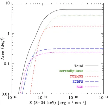
(3) The Astrophysical Journal, 854:33 (31pp), 2018 February 10. Zappacosta et al.. the NuSTAR data with archival low-energy data from Chandra and XMM-Newton. We perform broadband (0.5–24 keV) spectral modeling, characterize their spectral properties, and obtain a column density distribution, absorbed/CT fractions, and source counts, then compare them to predictions from population-synthesis models and past observational works. A companion paper (Del Moro et al. 2017, DM17) reports on the properties of the average X-ray spectra from all sources detected in the NuSTAR deep and medium survey fields. This paper is organized as follows. Section 2 presents the sample, with Sections 3 and 4 devoted to the data reduction and spectral characterization of the source properties, respectively. We then discuss the column density distribution (Section 5), fraction of CT AGN (Section 6), fraction of absorbed sources as a function of luminosity and redshift (Section 7), and source counts (Section 8). We discuss the results in Section 9, and present the conclusions in Section 10. Relevant notes on individual sources are presented in the Appendix. Throughout the paper, we adopt a flat cosmology with WL = 0.73 and H0 = 70 km s-1 Mpc-1. Errors are quoted at the 1s level and upper/lower limits at the 90% confidence level (c.l.). The X-ray luminosities are quoted in the standard (for NuSTAR survey studies) rest-frame 10–40 keV energy band.. 2.1. Medium-deep Survey Fields Given the 12¢ ´ 12¢ NuSTAR field of view, the survey fields (COSMOS, ECDF-S,and EGS) were observed with a mosaicing strategy whereby each neighboring pointing was shifted by half of a field of view. This tile arrangement produces homogeneous and continuous coverage in the deep central region with contiguous shallower edges. The main properties of these surveys are reported in Table 1. Despite NuSTAR being sensitive up to 79 keV, typical faint sources in the deep surveys are not detected to such high energies. In the extragalactic survey work to date, we have therefore only considered three energy bands: 3–24 keV (total), 3–8 keV (soft), and 8–24 keV (hard). Figure 1 reports the 8–24 keV sensitivity curves as a function of hard-band flux for all the fields. The sensitivities at 50% survey coverage are reported in Table 1. Notice that they are based on the assumption of an unabsorbed G = 1.8 power-law spectrum. This is an approximation that is reasonable for Compton-thin sources, given that above 8 keV their spectrum is minimally altered at the highest column densities (i.e., log [NH cm-2] 23). However, it may be somewhat inadequate for CT sources whose spectrum substantially deviates from this assumed spectral shape within this hard band. Therefore, it may give biased results in calculating the intrinsic distribution of physical quantities for the sampled AGN population. We account for this by correcting a posteriori for this bias (see Section 6 and Figure 11).. 2. Description of the Sample We draw our sample from the high-energy NuSTAR catalogs compiled for the COSMOS(Civano et al. 2015, C15), ECDF-S (Mullaney et al. 2015, M15), EGS (A. Del Moro et al. 2018, in preparation, DMIP) and serendipitous survey fields (L17). In order to have consistent catalogs, the same data-reduction tasks, mosaicing procedures, source-detection steps, photometry, and deblending algorithm were applied to all survey fields (see C15, M15, and Aird et al. 2015b for details). In the following, we briefly outline the source-identification procedure adopted in each catalog. The identification of the sources was consistently done through a SExtractor-based procedure on false probability maps generated on the mosaiced images accounting for the corresponding background maps in three energy bands (3–8, 8–24, 3–24 keV). No positional priors from previous low-energy X-ray surveys have been used in the source identification. Through simulated data, a proper threshold to set the significance of each source identification in each band has been adopted, and the final balance between completeness and reliability in each catalog has been chosen such there are no more than two or three possible spurious sources, down to the limiting flux in each catalog. Further details and description of the procedures regarding deblending, photometry, final catalog building, and association to lowenergy counterparts are reported in each catalog paper. For our purposes, in order to minimize obscuration bias, we selected objects with relatively bright fluxes in the hard 8–24 keV band. The fluxes adopted for this selection have been estimated from the 8–24 keV counts collected in 30″ apertures27 by the catalog papers, by assuming a power-law model with G = 1.8. Whenever possible, we complemented NuSTAR data with archival lower-energy data from Chandraand XMM-Newton.. 2.2. Serendipitous Survey Fields The serendipitous fields considered in this work consist of all fields analyzed as part of the serendipitous survey through 2015 January 1. This extends the sample presented by Alexander et al. (2013), and is a subset of the program presented in L17. The selection criteria adopted are reported in the following and constitute a slight modification to those employed in Aird et al. (2015b): 1. We minimize Galactic point-source contamination by requiring Galactic latitudes >20. 2. In order to emphasize fields where our serendipitous survey follow-up is currently more complete, we only consider fields accessible from the northern hemisphere by requiring declinations >-5. 3. We exclude fields with a large contamination from the primary targets by requiring <106 counts within 120″ of the aimpoint, and that primary targets contribute 6% to the extracted emission of the serendipitous source within the extraction region. After these cuts, the sky coverage of the serendipitous survey considered here amounts to »4 deg 2 (see Figure 1). Further survey details are reported in Table 1. It is worth noting that, despite the serendipitous survey having sensitivity better than COSMOS over a wider area and comparable faint source sensitivity to ECDF-S, it still has the disadvantage of having less multi-wavelength coverage. This usually translates to lower redshift completeness (from optical spectroscopy) and a poorer-quality X-ray coverage at low energies from Chandra and/or XMM-Newton (see L17).. 27. The fluxes reported in C15 are from 20″ apertures. They have been extrapolated to 30″ aperture fluxes by assuming a 1.47 constant conversion factor. This factor is obtained as the ratio between the fluxes in 30″ and 20″ apertures measured from the on-axis NuSTAR point-spread function.. 3.
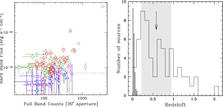
(4) The Astrophysical Journal, 854:33 (31pp), 2018 February 10. Zappacosta et al.. Table 1 Main Properties of the NuSTAR Extragalactic Surveys and Relative Catalogs Survey EGS ECDF-S COSMOS Serendipitousf. a. b. Pointings Exp.. Deepest Exp.. (Ms). (ks). (ks). 1.6 1.5 3.0 2.2. 50 45–50 20–30 20–1000. 400 360 90 970. Total Exp.. c. Pointing Layout. d. Area. 8×1 4×4 11×11 Random. Detected Sources. Sensitivity 50%e. (deg ). 3–24keV. 8–24keV. 3–24keV. 8–24keV. 0.24 0.31 1.73 3.91. 39 49 91 118. 14 19 32 38. 0.39 0.39 0.77 1.70. 0.35 0.45 0.93 1.35. 2. References DMIP M15 C15 L17. Notes. a Total exposure time devoted to the survey. b Average exposure times of the single pointings; notice that the serendipitous survey consists of pointings with a large range of exposure times. c Average exposure in the deepest field. d Tiling design of the survey. e Flux reached at 50% of the survey area coverage, in units of 10−13 erg s-1 cm-2 . f This is a subsample of the serendipitous survey sample presented in L17 (see Section 2.2).. focus of the following analysis. The redshift distribution is reported in the right panel of Figure 2, compared to the distribution of the 199 local sources detected by Swift-BAT in the energy range 15–55 keV (Burlon et al. 2011). NuSTAR, with its two orders of magnitude greater sensitivity, probes sources well beyond the local universe. Table 2 reports the position, spectroscopic redshift, Chandra and XMM-Newton counterparts, NuSTAR observation IDs, and NuSTAR survey for all 63 sources. When referring to the single sources, we use the catalog IDs listed in column 2 prefixed by ecdfs, egs, cosmos, and ser for sources from respectively the NuSTAR- ECDF-S, EGS, COSMOS, and serendipitous catalogs. Objects from the deep fields all have unique counterparts at lower energies from either the Chandra (Lehmer et al. 2005; Xue et al. 2011; Civano et al. 2012, 2016; Goulding et al. 2012) or XMM-Newton (Brusa et al. 2010; Ranalli et al. 2013) surveys of these same fields, with the exception of one source in the ECDF-S field (ecdfs5; this source has two possible counterparts, one at low and one at high redshift; see Table 2 and Appendix). A few sources have nearby potential contaminants (i.e., inside the NuSTAR extraction radius) in the deep survey fields. Contamination ultimately is unimportant or partially negligible in most cases, as discussed for the affected sources in the Appendix. For some cases (cosmos154 and cosmos181), we restrict the NuSTAR low-energy bound to 4–5 keV, where the contamination becomes less important. In a few other cases, the contamination is such that, within the uncertainties, it could potentially lower the true hard-band source flux also below the threshold flux used in our sample selection (cosmos107, cosmos178, and cosmos229). For the serendipitous survey sources, most have counterparts from at least Chandra or XMM-Newton, the exception being five sources (ser97, ser285, ser235, ser261, ser409; see Table 4) that have not yet been observed by these satellites.. Figure 1. Total and individual sensitivity curves as a function of the hard-band flux for the surveys included in our sample. Black solid curve is for the entire sample, magenta dotted–dashed is for EGS, blue long-dashed is for ECDF-S, red short-dashed is for COSMOS, and green dotted is for the serendipitous survey.. 2.3. Selected Sample The final catalogs consist of 91, 49, 39, and 118 objects, respectively, from the NuSTAR COSMOS, ECDF-S, EGS, and serendipitous survey. Of these, 32, 19, 14, and 38, respectively, are significantly detected in the hard-band, based on a maximum likelihood estimator (see C15, M15, Aird et al. 2015b, and L17 for details and the adopted thresholds). These objects are shown in Figure 2 (left panel), which displays the net 3–24 keV counts within a 30″ aperture versus their aperture-corrected photometry in the 8–24 keV energy band. From this combined sample, we select sources with hard-band flux S8 – 24 keV 7 ´ 10-14 erg s-1 cm-2 . We are sensitive to fluxes larger than this value in 80% of the surveyed area (see Figure 1). This subsample, corresponding to objects above the dashed line in Figure 2, includes a total of 31, 3, 5, and 24 objects from the four surveys, respectively, selected over a total area of ~6 deg 2 . The resulting sample of 63 sources is the. 3. Data Reduction 3.1. NuSTAR In order to perform a proper spectral analysis for these lowcount point-like sources (i.e., from tens to hundreds of counts; see Figure 2), we need to carefully account for: 1. the relatively uniform arcmin-scale NuSTAR point-spread function (FWHM= 18″; half-power diameter HPD=58″; Harrison et al. 2013); and 2. the spectrally variable and spatially dependent background 4.
(5) The Astrophysical Journal, 854:33 (31pp), 2018 February 10. Zappacosta et al.. Figure 2. Left panel: net counts in the full (3–24 keV) energy band from a 30″ aperture vs. the hard (8–24 keV) deblended aperture-corrected flux for the hard-band detected objects in the NuSTAR-COSMOS (red squares), NuSTAR-ECDF-S (blue triangles), NuSTAR-EGS (magenta diamonds), and NuSTAR-Serendip (green circles) catalogs. For the COSMOS sources, the flux has been extrapolated from the 20″ apertures reported in C15, assuming a constant conversion factor of 1.47 based on the on-axis NuSTAR point-spread function. The horizontal dashed line indicates the threshold value of 7 ´ 10-14 erg s-1 cm-2 defining our sample. Right panel: spectroscopic redshift distribution of our sample (open histogram) compared to the the 199 local sources studied by Swift-BAT in Burlon et al. (2011; dark gray, with normalization and histogram binning rescaled by a factor of 10). The arrow indicates the median redshift value for the sample (ázñ = 0.58) and the light gray region shows the interquartile range.. (for details, see Wik et al. 2014). In particular, the latter at <20 keV is strongly affected by stray light from unfocused CXB photons reaching the detectors through the open design of the observatory (called “aperture background”). Given the flux levels of the sources in our sample, it is necessary to maximize and carefully account for their contribution relative to the backgrounds (especially with respect to the spatially dependent “aperture background”). We therefore optimize the spectral extraction radius to maximize the signal-to-noise ratio (S/N) and, within the Poissonian uncertainties, the number of collected net counts. To do this, we started with the level 2 data products and simulated background maps where the latter were created using the software NUSKYBGD (Wik et al. 2014) as described in C15 and M15. The simulated background maps reproduce the “aperture background” across the FoV and the normalization of the total background in each observation. In detail, we used all the observations pertaining to a given source in order to determine the total counts in increasing circular apertures centered on the source position, calculating both source +background counts (S) from the event files and background counts alone (B) from the simulated maps. We then calculated the radial profile for the net source counts N (<r ) = S (<r ) N (< r ) . The radius for B (<r ) and S N (<r ) = N ( < r ) + 2B ( < r ) spectral extraction rex is chosen as the radius that maximizes the S/N profile and, within its 1s range, also maximizes N. In the few (nine for COSMOS and one for ECDFS) cases in which a source is blended with a nearby source (closer than 2 arcmin), we further reduced rex so that the source flux from the contaminating source is reduced, within the aperture, to levels of 5–6%. Table 4 reports rex values for all the sources in our sample.. We used the task “nuproducts” in NUSTARDAS v.1.4.1 with the NuSTAR calibration database (CALDB version 20150123) for the spectral extractions and the creation of relative response files. The background spectrum for each source spectrum was simulated from the best-fit models of the background across the detectors obtained with NUSKYBGD. This software performs iterative joint fits of the observed backgrounds across the field extracted in 3 arcmin apertures placed in each chip of each focal plane module. The joint modeling aims to determine the normalization of the different background components, and hence characterize them at the position of the source. The fits are performed using spectral models of the instrumental (continuum + line activation due to particle background), cosmic focused (CXB) and cosmic unfocused background (straylight) components, and information on their spatial dependence across the detectors. We checked each best fit to ensure that no significant spatial or spectral residuals were present. After this procedure, we are (in principle) able to wellreproduce the background spectrum at each position of the detector. We further verify this by creating backgroundsubtracted images and visually inspecting them for spatial gradients indicative of poor background modeling. As a final step, the best-fit spectral model is used by NUSKYBGD to simulate the background within the source extraction aperture, but using an exposure time multiplied by 100 to ensure high S/N. We then co-added spectra, simulated backgrounds and response files for each source and in each detector. Table 4 reports NuSTAR net counts and total exposure time collected for each source. 5.
(6) 6. Name. ID N a. Decl.. zb. IDC c. ID X d. NuSTAR Observation IDse. NuSTARJ100129+013636 NuSTARJ100249+013851 NuSTARJ100101+014752 NuSTARJ095815+014932 NuSTARJ095926+015348 NuSTARJ100055+015633 NuSTARJ100024+015858 NuSTARJ095840+020437 NuSTARJ100141+020348 NuSTARJ095918+020956 NuSTARJ100308+020917 NuSTARJ095857+021320 NuSTARJ100307+021149 NuSTARJ095817+021548 NuSTARJ100032+021821 NuSTARJ095902+021912 NuSTARJ095909+021929 NuSTARJ095957+022244 NuSTARJ100228+024901 NuSTARJ095945+024750 NuSTARJ100238+024651 NuSTARJ095908+024310 NuSTARJ100243+024025 NuSTARJ100204+023726 NuSTARJ095837+023602 NuSTARJ100232+023538 NuSTARJ095849+022513 NuSTARJ095848+022419 NuSTARJ100229+023223 NuSTARJ095839+022350 NuSTARJ100259+022033 NuSTARJ033136−280132. cosmos97 cosmos107 cosmos129 cosmos130 cosmos145 cosmos154 cosmos155 cosmos178 cosmos181 cosmos194 cosmos195 cosmos206 cosmos207 cosmos216 cosmos217 cosmos218 cosmos229 cosmos232 cosmos249 cosmos251 cosmos253 cosmos263 cosmos272 cosmos282 cosmos284 cosmos287 cosmos296 cosmos297 cosmos299 cosmos322 cosmos330 ecdfs5. 150.372537 150.705859 150.256432 149.564437 149.860885 150.233212 150.104087 149.668862 150.423842 149.826665 150.785979 149.738507 150.782581 149.573824 150.133457 149.761712 149.789727 149.990626 150.620155 149.941358 150.658422 149.785525 150.682309 150.520310 149.656383 150.635807 149.704281 149.700185 150.624855 149.662604 150.747792 52.901946. +1.610073 +1.647561 +1.797837 +1.825731 +1.896815 +1.942588 +1.982873 +2.077021 +2.063424 +2.165826 +2.154816 +2.222475 +2.197149 +2.263384 +2.305840 +2.320121 +2.324908 +2.378889 +2.817155 +2.797420 +2.780956 +2.719548 +2.673758 +2.623974 +2.600703 +2.593895 +2.420472 +2.405449 +2.539961 +2.397242 +2.342593 −28.025645. ecdfs20 ecdfs51 egs1 egs9. 53.032301 53.370361 214.400911 214.475905. −27.626858 −27.945068 +52.508258 +52.694030. cid1678 lid1688 cid284 lid961 cid209 cid1105 cid358 cid168 cid482 cid320 lid1646 cid329 lid1645 lid633 cid87 cid440 cid420 cid530 lid3218 lid545 lid484 lid549 lid492 lid294 lid1856 lid280 cid513 cid417 lid278 lid622 lid1791 103 100 301 712 37 294. 2021 5496 54490 5323 293 131 1 417 2608 5 5321 2 5370 54514 18 3 23 212 5014 5620 5114 5230 5400 7 2076 5133 126 135 5222 1429 5371 L L 358 L L L. 098001 101002 037002 038001 090001 012001 018001 062001 029001 030001 035002 023001 024001 029001 004001 005001 087001 040001 041001 050001 003001 004001 009002-B 109001 003001 111001 086001 020002 021001 026001 002001 003001 008001 002001 003001 008001 013001 014001 019001 067001 076001 077001-A 120001 077001 079001 118001 119001 120001 046002 046004 065002 082001 046002 116001 117001-B 118001 001002 001002 046002 046004 065002 116001 001002 002001 084001 113001 001003 001002. NuSTARJ033207−273736 NuSTARJ033328−275642 NuSTARJ141736+523029 NuSTARJ141754+524138. 0.104 0.694 0.907 1.509 0.445 0.219 0.373 0.340 0.125 1.157 1.470 1.024 0.582 0.707 1.598 0.345 0.378 0.931 0.213 1.067 0.212 1.317 0.669 0.519 0.735 0.658 1.108 0.375 0.432 0.356 0.044 0.141 1.957 0.976 0.841 0.987 0.464. NuSTARJ142047+525809. egs26. 215.196713. +52.969305. 0.201. 669. L. NuSTARJ142052+525630. egs27. 215.220076. +52.941858. 0.676. 622. L. NuSTARJ142027+530454. egs32. 215.113227. +53.081728. 0.997. 863. L. NuSTARJ023228+202349 NuSTARJ035911+103126 NuSTARJ051617−001340. ser37 ser77 ser97. 38.119089 59.798670 79.073788. +20.397218 +10.523951 −0.227904. 0.029 0.167 0.201. L L L. L L L. Catalog 099001 103001 060001 091001 063001 036002 030001 088002 051001 010001 111001 004001 113001 087001 027002 009002 009002 020002 120001 078001 121001 080001 121001 066001 083001 119001 002001 002001 118001 085001 115001 001003. 013001 013002 014001 014002 004001 004002 008001 008002 001002 001004 001006 001008 001002 001004 001008 002002 002003 002004B 002005 006002 006003 006004 006005 007001 007003 007005 007007 006002 006004A 006005 007001 007005 007007 007001 007003 007005 007007 008001 008002 008003 008004 60002048002 60002047006 60002047004 60061042002 60001044004 60001044002. COSMOS COSMOS COSMOS COSMOS COSMOS COSMOS COSMOS COSMOS COSMOS COSMOS COSMOS COSMOS COSMOS COSMOS COSMOS COSMOS COSMOS COSMOS COSMOS COSMOS COSMOS COSMOS COSMOS COSMOS COSMOS COSMOS COSMOS COSMOS COSMOS COSMOS COSMOS E-CDFS E-CDFS E-CDFS E-CDFS EGS EGS EGS EGS EGS. Serendip Serendip Serendip. Zappacosta et al.. R.A.. The Astrophysical Journal, 854:33 (31pp), 2018 February 10. Table 2 The Bright NuSTAR Hard-band Spectroscopic Sample.
(7) Name. ID N a. 7. R.A.. Decl.. zb. IDC c. ID X d. NuSTAR Observation IDse. Catalog. NuSTARJ061640+710811 NuSTARJ075800+392027 NuSTARJ081909+703930 NuSTARJ095512+694739. ser107 ser148 ser153 ser184. 94.167546 119.503085 124.789365 148.800066. +71.136661 +39.341045 +70.658570 +69.794361. 0.203 0.095 1.278 0.675. L L L L. L L L L. Serendip Serendip Serendip Serendip. NuSTARJ102345+004407 NuSTARJ102628+254417 NuSTARJ110740+723234 NuSTARJ112829+583151 NuSTARJ115912+423242. ser213 ser215 ser235 ser243 ser254. 155.938116 156.619145 166.919819 172.122122 179.802748. +0.735278 +25.738177 +72.542882 +58.530861 +42.545158. 0.300 0.827 2.100 0.410 0.177. L L L L L. L L L L L. NuSTARJ120613+495712 NuSTARJ121358+293608 NuSTARJ121425+293610 NuSTARJ122751+321222 NuSTARJ134513+554751 NuSTARJ143026+415959 NuSTARJ151508+420837 NuSTARJ151654+561744 NuSTARJ171309+573421 NuSTARJ181429+341055 NuSTARJ182615+720942 NuSTARJ204020−005609. ser261 ser267 ser273 ser285 ser318 ser335 ser359 ser363 ser382 ser401 ser409 ser451. 181.555033 183.494820 183.607905 186.964887 206.304766 217.610385 228.786883 229.225216 258.288435 273.621211 276.563078 310.087027. +49.953531 +29.602344 +29.603048 +32.206371 +55.797766 +41.999984 +42.143734 +56.295566 +57.572549 +34.181958 +72.161734 −0.936058. 0.784 0.131 0.308 0.733 1.167 0.352 0.289 1.310 0.243 0.763 1.225 0.601. L L L L L L L L L L L L. L L L L L L L L L L L L. 60002048010 60002048006 60002048004 60001131002 30001031005 30001031003 30001031002 80002092011 80002092009 80002092008 80002092007 80002092006 80002092004 80002092002 30001027006 60001107002 60002042004 60002042002 50002041003 50002041002 60001148004 60001148002 60061217006 60061217004B 60061217002 60061357002 60061335002 60061335002 60001108002 60002028002 60001103002 60061348002 30002039005A 30002039003 30002039002 60001137002 60001114002 60161687002 30001120005 30001120004 30001120003 30001120002. Serendip Serendip Serendip Serendip Serendip Serendip Serendip Serendip Serendip Serendip Serendip Serendip Serendip Serendip Serendip Serendip Serendip. The Astrophysical Journal, 854:33 (31pp), 2018 February 10. Table 2 (Continued). Notes. Identification name for each source. This is made from a prefix indicating the source parent catalog plus the ID from NuSTAR parent catalogs (Section 2). The prefixes of each parent catalog are cosmos for COSMOS, ecdfs for ECDF-S egs for EGS, and ser for the serendipitous survey. b All the redshifts are spectroscopic. They are taken from: Brusa et al. (2010; COSMOS), Lehmer et al. (2005), Xue et al. (2011) and Ranalli et al. (2013; ECDF-S), Nandra et al. (2015; EGS), and L17 (NuSTAR Serendipitous Survey). c Chandra IDs are from Elvis et al. (2009) and Civano et al. (2016; COSMOS, with prefix cid and lid respectively), Lehmer et al. (2005; ECDF-S), and Nandra et al. (2015; EGS). d XMM-Newton IDs are from Brusa et al. (2010; COSMOS) and Ranalli et al. (2013; ECDF-S). e To obtain the full NuSTAR observation IDs for the COSMOS, ECDF-S, and EGS fields, the six-digit survey identification numbers 60021, 60022, and 60023 must be prefixed, respectively. a. Zappacosta et al..
(8) The Astrophysical Journal, 854:33 (31pp), 2018 February 10. Zappacosta et al.. used both ACIS-S and ACIS-I detectors whenever available (see Table 3 for details). When multiple archival data sets were available, we chose the data closest in time to the NuSTAR observation, if available, in order to minimize source variability. Table 3 reports the selected observations for each source. We reduced the Chandra data using CIAO v.4.7 with28 CALDB v. 4.6.7. We re-processed the data using the CHANDRA_REPRO script to produce new re-calibrated level = 2 event files. The spectral extraction was done with the script SPECEXTRACT, which automates the creation of source and background spectral files and the relative ARF and RMF. The source and background spectral extractions were performed on user-selected circular and annular concentric regions, respectively, in order to maximize the source flux and avoid pointsource contamination to background measurements. We finally combined the resulting spectra using the FTOOLs script 29 ADDASCASPEC, available in HEASOFT v. 6.16, and produced combined RMFs and ARFs using the tasks ADDRMF and ADDARF. The resulting exposure times and collected net-source counts are reported in Table 4. For the XMM-Newton data, we used SAS v14.0.0.30 For each observation, we screened the event files for time intervals impacted by soft proton flares by adopting an observationdependent 10–12keV count-rate threshold (0.4 0.1 counts s-1 being the average and 1s standard deviation of the applied threshold), above which data were removed. For the spectral extraction and creation of response files, we followed the standard procedures outlined in the XMM-Newton science threads.31 We extracted events with pattern 4 for the PN camera and 12 for the MOS detectors. We combined the MOS1 and MOS2 spectra using the SAS task EPICSPECCOMBINE. For sources with more than one data set, we produced combined source spectra, background spectra, ARF, and RMF, as per the Chandra data. Exposure times and net-source counts for each source are reported in Table 4. For the EGS field, Chandra data products from Goulding et al. (2012) have been used. The spectral extraction, specifically carried out for this work,32 has been performed using SPECEXTRACT for each individual observation. Background regions were taken from annuli with 1.3 * r90,psf - 3.0 * r90,psf (with the latter being the radius enclosing 90% of the pointspread function) with other detected sources masked out. Spectra and backgrounds were combined for the different observations using COMBINE_SPECTRA in CIAO.. Table 3 Low-energy Observations Used for Serendipitous Sources Chandra. ID ser37 ser77 ser107 ser148 ser153 ser184. ser213 ser215 ser243 ser254 ser267 ser273 ser318 ser335. ser359 ser363 ser382 ser401 ser451. XMM-Newton. ObsID. Notes. ObsID. Notes. L L 10234 L L L L 10542 10543 10544 10925 11800 11104 L 12167 15077 15619 L L 14042 14042 L L L L L L L L L L. L L 1 L L L L 4 4 4 4 4 4 L 5 3, 5 3, 5 L L 1 1 L L L L L L L L L L. 0604210201 0604210301 0064600101 0064600301 0111220201 0406740101 0724810301 0657801901 0657802101 0657802301 L L L 0203050201 L L L 0744040301 0744040401 L L 0722610201 0111260101 0111260701 0212480701 0651850501 0724810201 0724810401 0764910201 0693750101 0111180201. L L L L 2 L 3 3 3 3 L L L L L L L 6 6 L L 3 L L L L 3 3 L L L. Notes. (1) Chandra/ACIS-I detector. (2) XMM-Newton/MOS data. (3) Observations chosen to be closest in time to the NuSTAR data. (4) The source is on the Chandra/ACIS-S2 chip. (5) The source is on the Chandra/ ACIS-S3 chip. (6) See Ricci et al. (2016) for details on data reduction and spectral extraction.. 3.2. XMM-Newton and Chandra For the ECDF-S and COSMOS fields, we employed all spectra reduced and extracted by previous works. Specifically, for the deep ECDF-S field, we used Chandra data reduced by Lehmer et al. (2005) and Xue et al. (2016), and extracted spectra following procedures discussed in Del Moro et al. (2014). For ecdfs20, which only has an XMM-Newton spectrum, the data reduction and spectral extraction are from Ranalli et al. (2013) and Georgantopoulos et al. (2013). For the COSMOS field, we use spectra reduced and extracted for XMM-Newton by Mainieri et al. (2007) and for Chandra by Lanzuisi et al. (2013), with the only exception being source cosmos330, for which a spectrum from the COSMOS-Legacy field has been used (Marchesi et al. 2016). For the serendipitous survey fields, we reduced and extracted the Chandra and XMM-Newton data. In the selection of archival observations, we only use data from observations in which CCD detectors are primary instruments (i.e., we exclude Chandra grating observations). In the case of XMM-Newton, we almost always only use data from PN, the exception being ser107, which was located in a CCD gap of the PN camera. For this source, we use the MOS data. For the Chandra data, we. 4. Data Analysis We performed the spectral analysis via XSPEC v.12.8.2 using the Cash statistic (Cash 1979) with the direct background subtraction option (Wachter et al. 1979). In the limit of a large number of counts per bin, the distribution of this statistic, called the W statistic (Wstat), approximates the c 2 distribution with N–M degrees of freedom (dof, where N is the number of independent bins and M is the number of free parameters). We performed all our modeling with spectra binned to five netcounts (i.e., background subtracted) per bin, with the exception 28 29 30 31 32. 8. http://cxc.harvard.edu/ciao4.7/ http://heasarc.gsfc.nasa.gov/docs/software/lheasoft/ https://www.cosmos.esa.int/web/xmm-newton/sas http://www.cosmos.esa.int/web/xmm-newton/sas-threads CIAO v.4.8 with CALDB v.4.7.0 has been used..
(9) The Astrophysical Journal, 854:33 (31pp), 2018 February 10. Zappacosta et al. Table 4 Spectral Extraction Parameters. NuSTAR FPMA. NuSTAR ID cosmos97 cosmos107 cosmos129 cosmos130 cosmos145 cosmos154 cosmos155 cosmos178 cosmos181 cosmos194 cosmos195 cosmos206 cosmos207 cosmos216 cosmos217 cosmos218 cosmos229 cosmos232 cosmos249 cosmos251 cosmos253 cosmos263 cosmos272 cosmos282 cosmos284 cosmos287 cosmos296 cosmos297 cosmos299 cosmos322 cosmos330 ecdfs5 ecdfs20 ecdfs51 egs1 egs9 egs26 egs27 egs32 ser37 ser77 ser97 ser107 ser148 ser153 ser184 ser213 ser215 ser235 ser243 ser254 ser261 ser267 ser273 ser285 ser318 ser335 ser359 ser363 ser382 ser401 ser409 ser451. NuSTAR FPMB. Chandra. XMM-Newton. net cts. expa. rexb. net cts. expa. rexb. net cts. expa. Ref.. net cts. expa. Ref.. 246 26 21 111 109 114 531 110 75c 86 82 149 58 45 44 500 56 75 23 74 71 239 110 158 38 88 27 78 167 114 131 82 149 170 180 453 593 294 614 267 104 290 80 4105 321 635 637 99 211 172 495 11 27 521 33 123 93 56 293 33 17 23 261. 57.1 52.8 71.5 49.6 103.2 100.1 104.8 97.8 95.0 73.1 48.7 46.6 49.7 51.5 114.4 98.6 98.6 111.8 52.0 78.0 52.9 76.7 106.4 83.1 52.6 111.7 45.6 45.6 110.7 99.1 52.8 89.5 192.6 185.8 149.4 302.8 400.5 300.2 390.4 49.1 27.3 120.8 127.6 38.7 142.5 943.6 94.3 59.4 123.1 69.2 90.2 22.4 20.4 20.4 23.2 67.7 49.2 23.9 224.7 49.4 21.3 32.3 95.1. 60 25 30 40 50 45 60 60 40 35 40 45 35 45 20 55 25 40 25 30 40 55 40 40 40 30 20 30 40 40 55 30 20 45 55 50 55 55 60 20 55 35 30 90 50 40 55 45 50 20 45 25 40 70 35 50 40 50 50 30 20 25 60. 268 21 27 103 77 119 534 67 55c 182 100 101 65 34 42 470 53 38 28 51 43 184 113 177 43 93 38 50 176 93 105 127 136 179 166 387 578 250 484 106 97 344 130 4299 327 1002 510 74 169 125 795 14 38 473 33 104 87 58 119 32 21 26 173. 57.0 52.7 71.5 49.5 103.1 99.5 104.1 97.7 94.9 99.1 48.7 46.6 49.6 51.4 114.3 98.5 98.5 111.7 51.9 52.1 52.8 76.5 106.2 82.9 52.5 107.1 45.5 45.5 110.5 99.0 52.7 89.1 192.6 185.6 205.5 354.2 399.6 251.3 389.6 30.1 27.3 120.6 127.4 42.4 221.7 974.7 94.1 59.3 122.8 69.1 142.1 22.4 20.3 20.3 23.1 68.0 49.1 23.8 110.1 50.0 21.3 32.2 98.7. 60 25 25 40 50 45 55 40 40 40 40 30 45 40 20 55 25 20 20 30 40 55 40 45 30 40 25 35 40 40 55 40 20 45 35 40 55 50 40 15 45 35 50 85 50 45 45 35 50 20 50 35 35 60 35 40 35 60 50 25 20 20 60. 392 L 46 L 603 185 5127 402 62 3174 L 1920 L 88 945 2170 316 240 L L L L L L L L 658 402 L L 183 532 1204 2079 2894 4195 2531 10696 5448 L 160 L L L L 5717 L 55 L 674 L L 45 1028 L L L L L L L L L. 47.1 L 186.7 L 189.5 189.4 184.8 93.2 92.4 185.9 L 91.5 L 140.5 188.5 88.9 133.9 185.6 L L L L L L L L 91.6 93.2 L L 147.9 240.3 357.9 245.6 197.5 719.0 683.9 683.9 683.9 L 31.7 L L L L 381.9 L 5.0 L 90.4 L L 5.0 5.0 L L L L L L L L L. 3 L 3 L 3 3 3 3 3 3 L 3 L 3 3 3 3 3 L L L L L L L L 3 3 L L 1 4,5 4,5 4,5 7 7 7 7 7 L 8 L L L L 8 L 8 L 8 L L 8 8 L L L L L L L L L. 675 73 54 1498 329 L 3520 218 99 2383 682 2957 175 104 821 3417 1096 115 138 721 191 514 189 2790 1159 946 893 1056 111 613 80 L 3743 L L L L L L 956 42 L 50d 6316 5 251 52 L L L 439 L L L L 129 996 151 898 190 158 L 5. 40.1 20.5 57.1 37.5 45.8 L 46.1 32.0 53.5 53.3 17.5 43.3 18.7 56.2 63.5 39.6 60.8 63.7 32.9 29.1 32.5 12.9 36.9 46.0 73.3 31.3 45.9 64.3 38.2 51.8 39.9 L 1862.2 L L L L L L 28.7 12.5 L 49.8d 10.9 5.8 21.2 11.3 L L L 36.5 L L L L 3.0 23.9 18.1 32.8 19.4 22.8 L 7.6. 2 2 2 2 2 L 2 2 2 2 2 2 2 2 2 2 2 2 2 2 2 2 2 2 2 2 2 2 2 2 2 L 6 L L L L L L 8 L L 8 8 8 8 8 L L L 9 L L L L 8 8 8 8 8 8 L 8. Notes. a Exposure time in ks. b Extraction radius in arcseconds. c Counts in the energy range 4.5–24keV. See the Appendix for details on this source. d MOS spectrum; the source falls in a chip gap in PN. References. (1) Marchesi et al. (2016), (2) Mainieri et al. (2007), (3) Lanzuisi et al. (2013), (4) Lehmer et al. (2005), (5) Xue et al. (2016), (6) Ranalli et al. (2013), (7) Goulding et al. (2012), (8) this work, and (9) data reduction as in Ricci et al. (2016).. 9.
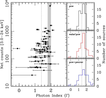
(10) The Astrophysical Journal, 854:33 (31pp), 2018 February 10. Zappacosta et al.. of sources with a low number of counts (i.e., 50 counts from both NuSTAR detectors), for which we resorted to a finer binning of one net-count per bin. The spectral modeling has been performed: (a) for the NuSTAR-only data, in the energy range 3–24 keV, assuming a power law, with absorption and reflection (Section 4.1), and (b) jointly together with XMM-Newton and Chandra over the broader 0.5–24 keV energy band, using more complex models (Section 4.2). Notice that, despite the spectral analysis being performed up to 24keV, on average, our spectra are sensitive to slightly lower energies. The median and semi-interquartile range for the highest energy bin in the FPMA and FPMB spectra are 19.6±3.0keV and 17.9±2.4keV, respectively. 4.1. NuSTAR Spectral Analysis For the NuSTAR-only analysis (3–24 keV), we first use a power-law model. We freeze the cross-calibration between FPMA and FPMB because, given the few percent level of accuracy measured by Madsen et al. (2015) and the limited counts of the majority of our spectra (up to a few hundreds) we do not expect to distinguish these small calibration levels (i.e., the statistical uncertainties exceed the systematic ones). The left panel of Figure 3 presents the power-law photon index Γ values plotted against the net counts in the 3–24 keV band. The Γ values are, on average, flatter than the canonical 1.8–2 values (e.g., Piconcelli et al. 2005; Dadina 2008) with a mean (median) of 1.5 (1.6). The distribution of Γ is reported by the black histogram in the right-upper panel. Spectra with fewer counts than the median have slightly flatter photon indices than high-count sources, áGlowñ = 1.4 0.2 compared to áGhighñ = 1.7 0.3. The average hardening of faint sources agrees with the shape of the CXB in approximately the same energy range (Marshall et al. 1980), as already found at lower energies (e.g., Mushotzky et al. 2000; Brandt et al. 2001; Giacconi et al. 2001). There is one notable outlier with a negative Γ value— the CT thick source in the COSMOS field reported by C15 (cosmos330 in Table 2). The average flat values of Γ point to a more complex spectral shape in the NuSTAR energy band. In order to identify a more suitable model that would bring the power-law photon indices to the canonical 1.8–2 values, we explored two modifications to the simple power-law model. We first allowed for low-energy photoelectric absorption by the circumnuclear interstellar matter, using the ZWABS model in XSPEC. Given the 3keV lower bound of the NuSTAR energy range, this model modification did not appreciably change the distribution of Γ, producing a median of 1.6 and only a few outliers (∼10% of the sample) at values much larger than 3 (see red dashed histogram in Figure 3). An alternative modification is the inclusion, beside the simple power-law component, of an additional cold Compton-reflection component to account for the disk/torus reflectors. This component is particularly important in the NuSTAR hard-energy band. We used the PEXRAV model (Magdziarz & Zdziarski 1995), which assumes that the reflector is an infinite slab with infinite optical depth illuminated by the primary power-law continuum, subtending an angle W = 2pR, where R is the reflection parameter. For a source of isotropic emission, W = 2p ; hence R=1. We tied both the photon index and the normalization of the reflection model to those of the primary power law and let R vary. In our modeling throughout the paper, we set this parameter in XSPEC to be negative; as for PEXRAV, this will switch on the. Figure 3. Left panel: 3–24keV net counts vs. photon index for the NuSTARonly joint fit derived using a power-law model (black dots). Right panels (from top to bottom): black, red, and blue histograms report the distribution for the power-law, absorbed power-law, and power-law plus reflection component models, respectively. Gray regions represent the canonical range of Γ values measured in the literature for the power-law component. The dotted line represents the 3–15keV slope of the CXB as measured by HEAO-1 (Marshall et al. 1980).. reflection-only solution as opposed to the reflection+powerlaw solution activated by positive values. Throughout the text, we quote the absolute value of the parameter. We left the abundance at its default solar value, cos q = 0.45 (i.e., inclination angle q ~ 63°, the default value in the model), and set the exponential cut-off (Ec ) for the incident power-law primary continuum at 200keV (as assumed by G07 and consistent with recent determinations by NuSTAR; see Fabian et al. 2015 for a compilation). This additional component shifts the mean and median photon index to higher values (G = 1.8 and G = 1.7, respectively), but at the cost of increasing the dispersion of the distribution (see blue histogram in Figure 3). There is no trend in the median Γ with the number of counts— except for the dispersion, with low-count sources having an interquartile range of 1.2, as opposed to high-counts sources having an interquartile range of 0.6. Histograms of the Γ distribution for the three models are reported in the right panels of Figure 3. 4.2. Joint Broad Band Analysis In order to improve the modeling and obtain tighter constraints on the spectral parameters, we added lower-energy data from XMM-Newton and Chandra, thereby extending the spectral range down to E = 0.5 keV (observed frame). Table 4 reports details on the low-energy data used for each source. We first consider an empirical model (hereafter called baseline model), expressed in XSPEC as: CONSTANT ´ WABS (POWERLAWsc. + ZGAUSS +. +. ZWABS. ´. POWERLAW. PEXRAV) ,. where POWERLAW represents the primary coronal component modified at low energies with photoelectric absorption (model 10.
(11) The Astrophysical Journal, 854:33 (31pp), 2018 February 10. Zappacosta et al.. ZWABS). and complemented at high energies with the addition of a cold Compton-reflection component (model PEXRAV). We further add a power law (POWERLAWsc ) at low energy to account, when needed, for residual low-energy flux for absorbed sources (hereafter called scattered component) consisting either of primary component flux scattered outside the nuclear absorbing region or of circumnuclear photoionized gas. At high energy, we add a line (ZGAUSS) to account for neutral FeKα emission at 6.4keV produced by the surrounding reflecting cold medium, and let its normalization free to vary. The entire model is modified by photoelectric absorption (WABS) from Galactic interstellar gas using values reported by Kalberla et al. (2005) at the position of each source. The CONSTANT accounts for instrument intercalibration and possible source flux variability, as well allowing for a crude accounting of possible contamination from blended sources inside differing extraction radii. We left the constant free to vary between satellites, but always tied between the two NuSTAR FPMs33 as done in Section 4.1. We left the slope and normalization of the scattered component free to vary. As in Section 4.1, we used the reflection-only component from PEXRAV and tied both Γ and normalization to the corresponding parameters of the primary component. Other PEXRAV parameters are set to the default values as reported in Section 4.1. In this way, our fits with the baseline model are performed with five free parameters. In case of a joint fit performed with one or two additional low-energy data sets, one or two intercalibration constants need to be accounted as additional free parameters, respectively. Furthermore, in the case of sources with a soft-excess component, two additional free parameters need to be considered for the slope and normalization of the scattered component. In order to speed up our modeling, which can be quite time-consuming using PEXRAV, the error estimation on all parameters was obtained with the reflection strength parameter R and calibration constants fixed to their best-fit values. For error estimation in R, we left only NH , Γ, and normalization of the primary powerlaw component free to vary. Best-fit spectral parameters are reported in Table 5, along with fluxes in the 8–24keV and 3–24keV bands, and 10–40keV unabsorbed and intrinsic coronal luminosities inferred from the best-fit baseline model (see Section 4.4 for details). Figure 4 shows broadband spectra for four sources, along with their best-fit model. For the few sources exhibiting extreme Γ values below 1.3 or above ∼2.5 or reflection parameters larger than ∼10, we redid the fits with Γ fixed to 1.8. These sources are cosmos129, cosmos232, cosmos253, cosmos282, ser285, ser77, and ser261. In three cases, mainly unabsorbed sources with high-quality spectra, the baseline parameterization in the soft- (ser148) and broadband (ser37, egs26) was inadequate. Indeed, in these energy ranges,. absorbed power-law models return slopes in the range G = 0.2–1.2 with very little absorption. We therefore further modified the absorbed primary power law by further applying absorption from a partial covering cold (ZPCFABS in XSPEC) or partially ionized (ZXIPCF) medium. Details on these sources are reported in the Appendix. 4.3. Absorption and Photon Index from the Primary Power Law The distribution of the measured Γ peaks at around 1.8–2, with a mean value of 1.89±0.26, as reported in Figure 5. Best-fit column density values range from 10 21 cm-2 to 1024 cm-2 . We have upper limits for 23 sources. Twenty are unabsorbed sources with NH upper limits <10 22 cm-2 . The two remaining sources have NH upper limits reaching into the heavily absorbed regime (~10 23–10 24 cm-2 ). These sources, ser285 and ser235, have low-count NuSTAR data and no lower energy data available. For only one source with NuSTAR-only data (ser409) can we not constrain its NH value even when fixing G = 1.8. For 17 sources, ∼27% of the sample, we measure NH 1023 cm-2 . Two sources (∼3% of the sample), cosmos330 and ser261, exhibit CT column densities. The former is the CT AGN discovered by C15. Figure 5 shows Γ as a function of intrinsic NH . Error bars in Γ tend to be larger for obscured sources (i.e., NH 10 22 cm-2 ). 4.4. Luminosity in the 10–40keV Energy Band In the last two columns of Table 5, we report the 10–40keV luminosities from the baseline model. They are unabsorbed luminosities (L u,X , penultimate column) and intrinsic luminosities (L i,X , last column). The unabsorbed luminosity is estimated by simply removing the Galactic and intrinsic absorption components from the best-fit baseline model. The intrinsic coronal luminosities are computed from the unabsorbed coronal power-law component by simply removing the reflection contribution to the best-fit baseline model. The uncertainties in L i,X due to parameter degeneracy in our modeling are estimated by fitting the baseline model with R fixed to its lower and upper error bounds. In the context of the baseline parameterization, L i,X is supposed to reflect more closely the true X-ray radiative output of the primary (direct) X-ray emitting nuclear source. Notice, though, that the planar geometry assumed in PEXRAV is an approximate description of the cold reflector—which, according to unification schemes, has a toroidal geometry. In any case, in the 10–40keV band, the additional reflection contribution can become relevant compared to the intrinsic coronal one, especially for sources with low luminosity and large reflection strengths. Including the reflection term in the luminosity calculation may lead to a “double counting” of the intrinsic X-ray radiative output. Indeed, in this case, the estimate of L u,X would include both the primary coronal power-law component and the primary coronal photons reflected from the circumnuclear material back to the observer. This overestimation of the intrinsic luminosity is negligible (10%–30% for R=1–6) in the 2–10keV band where the reflection component is a few percent of the primary emission. The upper panel of Figure 6 shows, for the 10–40keV band, the overestimate of the “unabsorbed luminosities,” including the reflection component compared to the intrinsic. 33. For the 58 sources with low-energy spectral data, the difference between the estimated best-fit constants is reasonably low, being smaller than a factor of ∼2 for the majority of the sources (50). Four sources (cosmos129, cosmos229, cosmos297, and ser77) show variations larger than a factor of 2–3 in both XMM-Newton and NuSTAR, clearly pointing to source variability as the main cause of discrepancy. The remaining four sources, cosmos249, cosmos263, ser148, and ecdfs5, have variations by factors of 2–4, with the latter showing the largest variation that is possibly due to contamination from a nearby source (see the Appendix for details).. 11.
(12) The Astrophysical Journal, 854:33 (31pp), 2018 February 10. Zappacosta et al.. Table 5 Best-fit Parameters for Baseline Model NuSTAR ID. stat. dof. Γ. log NH a. R. S8 – 24 b. S3 – 24 b. log L u,X c. log L i,X d. cosmos97 cosmos107 cosmos129 cosmos130 cosmos145 cosmos154 cosmos155 cosmos178 cosmos181 cosmos194 cosmos195 cosmos206 cosmos207 cosmos216 cosmos217 cosmos218 cosmos229 cosmos232 cosmos249 cosmos251 cosmos253 cosmos263 cosmos272 cosmos282 cosmos284 cosmos287 cosmos296 cosmos297 cosmos299 cosmos322 cosmos330 ecdfs5 ecdfs20 ecdfs51 egs1 egs9 egs26e egs27 egs32 ser37f ser77 ser97 ser107 ser148f ser153 ser184 ser213 ser215 ser235 ser243 ser254 ser261 ser267 ser273 ser285 ser318 ser335 ser359. 257.1 19.0 16.0 256.1 150.6 76.3 788.7 143.9 38.0 581.2 139.3 547.4 57.6 23.8 321.3 674.8 231.4 62.3 23.4 138.0 49.5 160.8 81.9 390.2 184.4 162.3 202.5 272.9 99.1 151.9 81.2 151.7 695.6 318.2 220.1 438.4 424.4 424.9 458.6 223.3 64.9 93.7 27.6 1338.4 98.3 461.2 183.5 36.8 64.8 152.6 261.7 15.5 14.8 221.0 7.7 63.9 135.6 23.8. 262 16 24 247 170 70 792 127 45 587 138 571 50 41 267 695 221 76 27 127 52 153 68 377 186 164 234 247 71 137 81 104 717 229 268 459 429 411 462 219 66 95 38 1260 93 538 183 35 56 145 260 15 14 276 9 56 189 44. +0.08 2.070.08 +0.71 1.740.52 1.8 +0.06 1.870.05 +0.11 1.71-0.08 +0.38 1.800.21 +0.01 2.030.02 +0.11 1.460.08 +0.16 2.100.14 +0.03 1.79-0.02 +0.06 1.610.08 +0.03 1.770.02 +0.16 1.700.07 +0.16 1.750.15 +0.07 1.850.07 +0.02 1.900.02 +0.05 2.040.03 1.8 +0.36 1.980.61 +0.07 2.370.05 1.8 +0.05 1.880.03 +0.16 1.35-0.14 1.8 +0.08 2.050.09 +0.08 2.330.08 +0.09 2.150.07 +0.10 1.98-0.07 +0.06 2.160.09 +0.10 1.960.08 +0.55 1.570.57 +0.08 1.900.07 +0.05 1.990.07 +0.06 1.980.05 +0.04 1.840.05 +0.06 1.800.04 +0.05 1.560.03 +0.02 2.300.02 +0.03 1.660.03 1.8 1.8 +0.32 2.250.18 +0.36 1.480.23 +0.02 2.510.01 +0.26 1.84-0.19 +0.03 1.730.02 +0.14 1.960.15 +0.06 1.970.08 +0.37 1.790.10 +0.11 1.35-0.10 +0.08 2.280.11 1.8 +0.26 2.130.23 +0.04 1.85-0.03 1.8 +0.15 2.410.08 +0.08 1.690.03 +0.29 1.460.20. +0.04 22.620.04 +0.29 23.630.30 +0.11 23.840.07 <21.41 +0.06 21.970.06 +0.09 23.55-0.08 <20.09 +0.24 21.000.82 +0.09 23.91-0.09 <20.93 +0.21 21.480.50 <20.89 <21.46 +0.23 23.780.26 +0.05 22.420.05 <20.17 <20.51 +0.06 23.410.06 +0.14 23.560.18 <21.17 +0.08 22.680.08 <21.32 +0.12 22.620.11 <20.39 +0.07 21.870.06 <21.13 <21.36 +0.05 21.990.04 +0.10 23.670.05 +0.06 21.740.07 +0.11 24.130.21 +0.22 20.870.51 +0.02 23.020.03 <21.20 +0.31 20.930.64 +0.02 22.720.02 +0.12 21.060.16 <20.56 +0.09 21.620.08 <20.58 +0.09 21.930.07 +0.24 23.060.22 +0.27 23.210.18 <19.89 +0.27 23.420.32 +0.20 20.88-0.22 +0.13 23.330.12 <21.71 <24.25 +0.05 23.020.05 +0.05 22.98-0.06 +0.51 24.610.32 <21.74 <20.87 <23.99 <21.79 <20.82 +0.18 22.560.13. +1.75 5.891.41 <0.91 <0.32 +0.36 0.390.18 +1.64 0.83-0.73 <0.34 +0.27 1.240.38 <1.96 +0.84 0.760.37 +0.15 0.38-0.15 +0.51 0.310.22 +0.16 0.230.13 +4.84 3.881.56 +1.33 1.971.39 <0.40 +0.30 1.170.11 +0.67 2.710.61 +0.27 0.580.30 <0.95 +0.88 1.170.49 +5.19 4.991.43 +0.17 0.110.10 +0.39 0.020.00 +0.18 0.420.18 +1.66 1.300.84 +1.01 1.240.54 +1.06 1.57-0.80 +2.11 1.550.94 +0.20 0.280.21 +1.67 2.581.08 +0.30 0.220.17 +11.26 3.172.09 +0.15 0.740.15 +0.93 1.050.60 +0.47 0.240.12 <0.28 <0.68 +0.21 1.060.31 <0.07 +0.55 1.780.84 +1.05 2.000.95 <1.40 <4.45 +0.41 2.630.36 <1.14 <0.10 +0.76 1.370.53 <16.72 <0.70 <0.74 +0.74 1.900.62 +0.95 0.370.29 +23.63 4.093.26 <0.19 <17.31 +0.76 0.560.30 <1.10 <13.89. 3.8 0.9 0.5 1.6 0.7 1.6 3.3 0.7 1.0 1.7 2.4 2.3 2.0 1.0 0.5 3.6 0.8 0.7 1.0 0.8 1.4 1.7 1.1 1.5 0.9 0.7 0.8 1.3 1.7 1.1 3.6 1.2 1.1 0.7 0.8 1.3 1.4 0.9 0.8 17.7 3.6 1.7 1.4 47.5 1.1 0.9 5.5 0.9 1.2 3.3 3.7 0.9 1.6 11.8 0.9 1.2 1.4 2.2. 5.4 1.3 0.7 2.5 1.0 2.1 5.3 1.0 1.2 2.6 3.7 3.6 2.7 1.2 0.9 5.5 1.1 0.9 1.4 1.3 1.8 2.8 1.6 2.3 1.4 1.2 1.3 2.0 2.3 1.5 3.8 1.8 1.6 1.1 1.3 2.2 2.0 1.5 1.4 23.7 5.2 3.1 1.9 85.7 1.8 1.5 7.5 1.5 2.0 4.6 5.9 1.0 2.8 21.1 1.4 2.2 2.3 3.2. 43.2 44.4 44.4 45.4 43.8 43.5 44.3 43.6 42.8 45.2 45.5 45.2 44.5 44.4 45.0 44.3 43.7 44.5 43.3 44.8 43.4 45.3 44.4 44.3 44.4 44.2 44.8 43.9 44.2 43.8 42.6 43.0 44.8 44.5 44.7 44.1 43.4 44.4 44.7 42.7 43.6 43.4 43.4 44.1 45.1 44.3 44.3 44.5 45.6 44.4 43.6 44.6 43.0 44.7 44.4 45.1 43.9 43.9. +0.03 42.620.04 +0.00 44.360.20 +0.00 44.420.04 +0.08 45.140.19 +0.08 43.580.20 +0.00 43.510.02 +0.01 44.060.03 +0.00 43.550.21 +0.05 42.690.00 +0.04 44.94-0.04 +0.12 45.330.26 +0.03 45.040.05 +0.08 43.850.33 +0.14 43.900.06 +0.05 44.91-0.21 +0.00 44.020.02 +0.00 43.200.00 +0.04 44.270.03 +0.00 43.300.03 +0.06 44.310.22 +0.03 42.840.15 +0.04 45.23-0.09 +0.00 44.390.06 +0.00 44.170.00 +0.17 44.020.25 +0.02 43.840.03 +0.08 44.220.07 +0.04 43.58-0.04 +0.02 44.090.09 +0.03 43.320.03 +0.01 42.520.00 +0.03 42.560.04 +0.03 44.460.03 +0.02 44.190.03 +0.01 44.570.03 +0.00 44.13-0.03 +0.00 43.370.09 +0.01 44.000.01 +0.00 44.710.01 +0.06 42.480.05 +0.03 43.290.03 +0.00 43.390.11 +0.00 43.340.18 +0.02 43.800.03 +0.00 45.110.20 +0.00 44.350.01 +0.06 44.050.07 +0.06 44.290.04 +0.00 45.650.28 +0.00 44.430.09 +0.04 43.330.04 +0.14 44.410.19 +0.06 42.520.13 +0.00 44.670.04 +0.27 44.090.89 +0.05 44.740.05 +0.01 43.820.05 +0.00 43.900.18. 12.
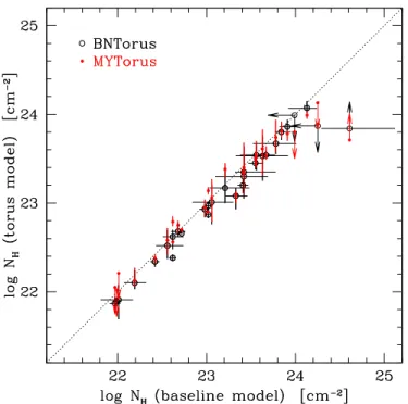
(13) The Astrophysical Journal, 854:33 (31pp), 2018 February 10. Zappacosta et al. Table 5 (Continued). NuSTAR ID. stat. dof. ser363 ser382 ser401 ser409 ser451. 129.4 40.7 31.6 33.8 52.2. 205 42 31 30 66. Γ. log NH a. R. S8 – 24 b. S3 – 24 b. log L u,X c. log L i,X d. +0.06 1.640.07 +0.24 1.880.20 +0.20 1.870.18 +0.11 1.680.06 +0.61 1.810.10. +0.14 21.670.26 +0.13 22.190.12 +0.16 22.010.20 L +0.36 23.420.10. <1.56 +8.43 0.750.72 <12.95 +2.99 0.710.62 <1.11. 1.2 0.9 0.9 0.9 1.4. 1.9 1.5 1.5 1.3 2.1. 45.1 43.3 44.5 44.9 44.4. +0.00 45.100.07 +0.02 43.180.16 +0.10 44.330.22 +0.17 44.580.51 +0.00 44.410.15. Notes. a NH in units of cm-2 . b Units of 10−13 erg s-1 cm-2 . c Unabsorbed luminosity in the 10–40keV energy range in units of erg s-1. See Section 4.4 for details. d Intrinsic luminosity in the 10–40keV energy range in units of erg s-1. Errors highlight the uncertainty associated with the reflection component modeling. See Section 4.4 for details. e For this source, we further added a partial covering absorber by partially cold material (zpcfabs in XSPEC). See the Appendix for further details. f For this source, we further added a partial covering absorber by partially ionized material (zxipcf in XSPEC). See the Appendix for further details.. luminosities derived from the unabsorbed primary component only. In the lower panel, we report the ratio between these two quantities in order to quantify better the level of overestimation. Here, L u,X can be larger by factors up to ∼2–4 and the majority of those sources are those with best-fit R > 1 (red diamonds) at low luminosity (i.e., L i,X 2 ´ 10 44 erg s-1 ). This is due to an induced dependence between R and luminosity; if not accounted for, this may lead to a biased view of the relationship between luminosity and reflection strength (see Section 4.5.1 and Figure 8, bottom panels). Notice that few sources at higher luminosities (2 ´ 10 44 erg s-1 ) have overestimates of a factor of ∼2, even though they have low reflection strengths (i.e., R < 1). This is due to the fact that the L u,X L i,X ratio in the observed 10–40keV energy range is an increasing function of the redshift34 and our sample, selected in flux, contains higher-luminosity sources, on average, at higher redshifts. In order to keep the baseline parameterization simple and suitable for low S/N spectra, we did not include a Comptonscattering term, which can become important for the most obscured sources. This may lead to an underestimate of the true luminosity for the most obscured sources. We compared our unabsorbed values with the best-fit values obtained by adding a Compton-scattering term parameterized with CABS for the COSMOS sources with log (NH cm-2) 24, i.e., those for which we have the best-quality broadband data. We obtained larger luminosities, on average, with values ranging from <0.1 dex for the less obscured sources up to ∼0.4dex for the most obscured ones. However, CABS approximates the Compton scattering by only accounting for the scattering of the photons outside the beam and neglecting photons reflected by surrounding material into the line of sight. Hence, more appropriate luminosity values may be estimated by accounting for the geometry of the obscurer. For this reason, we compared our values with those obtained with the torus modelings employed in Section 4.6, which self-consistently account for Compton-scattering effects due to the toroidal geometry of the obscurer. We found that, in the range log (NH cm-2) » 23–24.5, the 10–40keV luminosity is underestimated, on average, by at most ∼0.1dex, with only two exceptions in our sample: cosmos129 and ser261. These sources are among the. most obscured sources in our sample; for them, we have found L u,X underestimated by 0.2dex and 0.3–0.4dex, respectively. No significant difference is found for less obscured sources. 4.5. The Reflection Component We next estimate the significance of the reflection component in our sources. We first evaluated whether, for the obscured sources (log [NH cm-2] 22), the absorbed spectral shape could be better modeled in the context of a CT scenario in which the primary continuum is completely suppressed and where the only dominant component other than the soft residual scattered one is the pure cold reflection component. Hence, we evaluated a reflection-dominated spectrum obtained by removing the absorbed primary power-law component from the baseline model. Because we are not using c 2 statistics, we are not able to use an F-test to evaluate the significance of the baseline model over the simpler reflection-dominated one. We therefore based our evaluation on the presence of: (1) a reasonable input power-law photon index for the PEXRAV component of the best-fit parameterization of the reflectiondominated model; (2) a large fraction of scattered flux at low energies for the baseline model35; (3) the presence of an FeKα emission line with a large equivalent width (EW 1 keV); and (4) large residuals for the best-fit parameterization. Based on these criteria, we did not find clear cases of sources deviating from the baseline model or significantly better parameterized by a reflection-dominated model. Similarly, we did not find scattered fractions in excess of a few percent, the value that is typically found in heavily obscured sources (e.g., Lanzuisi et al. 2015). Moreover, only for cosmos181 did we obtain Fe Ka EW ~ 1 keV. Other sources show more moderate EWs. We therefore are unable to discriminate between the two models. 4.5.1. Reflection as a Function of Obscuration, Slope, and Luminosity of the Primary Emission. We measured R for all the sources (see Table 5 column 6) and obtained upper limits for 23 sources. We considered all the. 34. 35. Indeed, the redshift progressively shifts to lower energies (i.e., outside the band) portions of the spectrum where the decreasing primary component still significantly contributes to the total flux.. That is, if we are modeling an intrinsic reflection-dominated source with the baseline model, we obtain an overestimate of this quantity. To check for this, we tied Γ of the scattered component to the primary one.. 13.
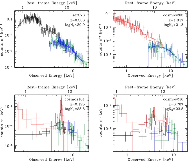
(14) The Astrophysical Journal, 854:33 (31pp), 2018 February 10. Zappacosta et al.. Figure 4. Examples of broadband spectra for four sources with best-fit baseline models (solid lines). Black, red, green, and blue spectra refer to Chandra, XMMNewton, NuSTAR-FPMA, and NuSTAR-FPMB, respectively. Upper/lower spectra are for unabsorbed/absorbed sources. Spectra on the left/right are for sources with redshifts lower/higher than ázñ.. best-fit values with R < 0.01 as upper limits. In Figure 7, we report the distribution of R in bins of 0.5dex.36 We investigated how reflection correlates with obscuration and luminosity for the whole sample. Figure 8 presents the reflection parameter as a function of column density (top-left panel) and unabsorbed and intrinsic 10–40keV luminosity (bottom panels). The color of each point corresponds to redshift, with the redder colors representing the more distant sources. Because ours is a flux-selected sample, more distant (i.e., redder) sources in the R –LX plane correspond to more luminous, less obscured sources (see R –NH plane). There is an apparent tendency for obscured and luminous sources to have, on average, maximum R values smaller than unobscured and less luminous sources. We investigated and quantified these trends by: (1) computing the Spearman’s rank correlation coefficient (ρ) for. censored data using the ASURV package v.1.2 (Lavalley et al. 1992; Feigelson & Nelson 1985; Isobe et al. 1986) and (2) calculating the median áRñ and its interquartile range (IQR) for the entire sample and the obscured/unobscured and luminous/ less luminous subsamples (the separation between the latter being dictated by the median luminosities of the sample, log [áL i,Xñ erg s-1] = 44.06 and log [áL u,Xñ erg s-1] = 44.35). For the latter, we accounted for measurement errors and upper limits in R, log (NH cm-2), and log L i,X as follows: we performed 10,000 realizations of the sample, each time with respective Gaussian and uniform randomization for each of the parameter best-fit values37 and the upper limits. In the case of R and log NH , the latter were randomized from their 90% upper value down to a fixed minimum value of R=0.01 and log (NH cm-2) = 20 . For each realization, we computed the median value and IQR, and adopted the averaged values over all the realizations as representative for the sample. The. 36 Notice that the derived R values are obtained by fixing the inclination angle (qincl ) for the reflector to qincl ~ 63 (default in Xspec). Assuming lower/larger inclination angles will decrease/increase R. For instance, fixing qincl = 30 (qincl = 85) would lower (increase) our reported R by 50% (a factor of 2–3).. 37. We assumed a symmetric distribution centered on the parameter value with 1σ standard deviation as the mean of the lower and upper error bars.. 14.
Figure
+7


Documento similar