A pedagogical Approach to the Aharonov Bohm effect
45
0
0
Texto completo
(2) 1. INTRODUCTION....................................................................................................................... 1 1.1 Classical mechanics approach ............................................................................................. 2 1.2 Magnetic field, vector potential and gauge symmetry ...................................................... 2 1.3 Quantum mechanics approach: The Aharonov-Bohm effect ............................................. 3. 2. AIMS OF THE PRESENT WORK ................................................................................................ 7. 3. ROLE OF SYSTEM TOPOLOGY ON THE AHARONOV BOHM EFFECT ........................................ 7 3.1 Zero magnetic field acting upon the electron. ................................................................. 9 3.2. Non-zero magnetic field acting upon the electron ........................................................ 10. 4. SYMMETRY INFLUENCE ON THE AHARANOV BOHM EFFECT .............................................. 12. 5. ROLE OF THE MAGNETIC FLUX ON THE AHARONOV BOHM EFFECT.................................... 12 5.1 Opposite magnetic fluxes of equal magnitude .............................................................. 12 5.2 Opposite magnetic fluxes of different magnitude ......................................................... 13. 6. RESULTS ................................................................................................................................ 14 6.1 Aharonov Bohm effect: magnetic flux centered at the origin of coordinates ............... 15 6.2 Role of the system topology .......................................................................................... 19 6.3 Symmetry influence ....................................................................................................... 23 6.4 Role of the magnetic flux ............................................................................................... 28. 7. CONCLUSIONS....................................................................................................................... 29. 8. BIBLIOGRAPHY ...................................................................................................................... 30. 9. APPENDIX .............................................................................................................................. 31.
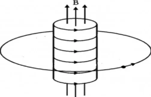
(3) Abstract We carry out a pedagogical approach to the Aharonov Bohm effect. To this aim, we employ the Comsol multiphysics program package to calculate the energy spectra of twodimensional quantum ring systems. We show that the Aharonov Bohm takes place when the system has an “interior” (i.e., non-trivial topology) pierced by a magnetic field. In addition, we show that the symmetry of the system affects the energy spectra but not the presence/absence of the Aharonov Bohm effect. Finally, we demonstrate that it is the total field flux and not the vector potential what influences the system.. 1. INTRODUCTION In 1959 Y. Aharonov and D. Bohm showed that an electron can be influenced by potentials even if no fields act upon it [1]. In classical mechanics, the fundamental equations of motion are expressed in terms of the magnetic field so the dynamics of a particle will not be affected when no field acts upon it. The magnetic field, though, can be derived from the vector potential. All the same, in classical mechanics the vector potential is viewed as a mere mathematical tool, with no physical meaning, just used to define the field, which is the observable quantity. Nonetheless, in quantum mechanics the canonical formalism is necessary and therefore the potentials cannot be eliminated from the equations of motion. As we will see, the quantum Aharonov Bohm effect has its roots on this fact. In order to introduce the Aharonov Bohm effect, let us consider the following simple experimental set up (figure 1) in which a charged particle, like an electron, is travelling around a solenoid describing a close path. The solenoid produces a magnetic flux so that there is magnetic field along the z axis different from zero outside the solenoid but that vanishes outside it. B ≠0 { inside Boutside = 0 Therefore, the magnetic field acting upon the particle is zero.. Figure 1: Experimental set up: a charged particle is travelling around a solenoid describing a close path. The solenoid creates a magnetic field inside the solenoid.. A pedagogical approach to the Aharonov Bohm effect. Page 1.
(4) We may ask the following basic question: Is the dynamics of the particle affected by the magnetic field inside the solenoid? Two different approaches can be taken in order to answer this question: a classical mechanics and a quantum mechanics one.. 1.1 Classical mechanics approach From a classical mechanics point of view, a force is necessary in order to affect the dynamics of a particle. This force is the Lorentz force in the presence of a magnetic field B: ⃗⃗) (1) 𝐹⃗ = 𝑒(𝑣 × 𝐵 However, the charged particle in the setup of figure 1 moves in the region where the magnetic field is zero. Therefore no net Lorenz force acts upon it. So, according to classic mechanics, its dynamics is not affected by the magnetic field of inside the solenoid. This is so because in Classic mechanics, the fundamental equations of motion can be expressed in terms of the field alone. The vector potential may appear or not in the equations, but it is considered as an auxiliary potential, not a real physical magnitude. Only the field is real. On the other hand, in the quantum mechanics formalism the use of the vector potential is unavoidable. Before introducing the quantum mechanics approach, we will give a little of insight into the relationship between magnetic field and vector potential. 1.2 Magnetic field, vector potential and gauge symmetry The magnetic field can be visualized as lines that show the direction and the strength of the magnetic field. They depart from the North Pole to the South Pole in a magnet, forming a close loop:. Figure 2: Magnetic field lines produced by a magnet.. The number of lines entering an imaginary surface on the magnet is equal to the number of lines leaving that surface (see figure 2). From a mathematical view this means that the divergence of the magnetic field is equal to zero: ∇ ∙ 𝐵 = 0 (2) That is to say, that there are no magnetic monopoles. But a vector calculus property says that the divergence of the curl of any vector A is always zero: A pedagogical approach to the Aharonov Bohm effect. Page 2.
(5) ∇ ∙ (∇ × 𝐴) = 0 (3) Therefore, the magnetic field can be defined as the curl of some vector A: 𝐵 = ∇ × 𝐴 (4) Where A is referred to as the vector potential. Now suppose some vector potential A1 to which the gradient of a scalar χ is added to form a new vector A: 𝐴 = 𝐴1 + ∇𝜒 (5) The magnetic field will be equal to the sum of the curl of A1 plus the curl of the gradient: 𝐵 = 𝛻 × 𝐴 = 𝛻 × 𝐴1 + 𝛁 × (𝛁𝝌). (6). However, the curl of a gradient is always zero: 𝛁 × (𝛁𝝌) = 𝟎 (7) Then, the magnetic field is equal to the curl of the original vector A1. We see that it is unaffected by the change introduced in the vector potential. This means that different vector potentials can be employed to describe a given magnetic field, just by adding different gradients. This property is referred to as gauge symmetry. The vector potential is a gauge dependent magnitude. The observable variables, like the field, should be gauge invariant, i.e., not affected by it. In other words, the vector potential can have a gauge-dependent definition, cannot be measured and thus it is not considered a physical quantity. Only gauge invariant variables like the magnetic field are real physical quantities. The equations of motion in classic mechanics are written in terms of the fields and the vector potential is considered a mere auxiliary mathematical tool. For a more in depth learning of gauge symmetry, the book “An elementary Primer for Gauge Theory” [2] is accessible to both scientists and students with only a background in quantum mechanics.. 1.3 Quantum mechanics approach: The Aharonov-Bohm effect We rely now on quantum mechanics to answer the question proposed in section 1: is the charged particle affected by the magnetic field inside the solenoid? Let us first derive the Hamiltonian of an electron in the presence of a magnetic field.. A pedagogical approach to the Aharonov Bohm effect. Page 3.
(6) a) Hamiltonian for an electron in the presence of a magnetic field If the dynamics of the particle is affected by the magnetic flux inside the solenoid, then this change will be reflected in the energy of the particle. The operator associated to the energy of the system is the Hamiltonian. For a free particle, the Hamiltonian is written in terms of the linear momentum operator 𝑝̂ : H=. p̂2 ; 𝑝̂ = −𝑖ћ∇ (8) 2m. Where m is the mass of the particle. In the presence of a magnetic field, the vector potential appears in the Hamiltonian (see Appendix 1). The Hamiltonian of a charged particle in the presence of a magnetic field results to be: [3] H=. (p̂ − eA)2 2m. (9). Where e is the charge of the particle and A is the vector potential. In the case of an electron (e=-1), the Hamiltonian takes the form: H=. (p̂ + A)2 2m. (10). If the square binomial is expanded: 𝐻=. 𝑝̂ 2 + (𝑝̂ 𝐴 + 𝐴𝑝̂ ) + 𝐴2 , (11) 2𝑚. and the momentum operator is explicitly written (𝑝̂ = −𝑖ћ∇) then: H=−. ћ2 2 iћ A2 (𝛁𝐀 + 𝐀𝛁) + 𝛻 − 2m 2m 2m. (12). In general, the nabla operator, ∇, and the vector potential , A, do not commute. However, the vector potential gauge symmetry allows choosing a vector potential with zero divergence: ∇ ∙ 𝐴 = 0 (13) This gauge is referred to as Coulomb gauge. When the divergence of the vector potential is zero, then A and 𝑝̂ commute. Then: ∇A + A∇= 2A∇ (14) In this case, the general formula for the Hamiltonian of an electron in the presence of a magnetic field, in terms of the vector potential, is: H=−. ћ2 2 iћ A2 𝛻 − A∇ + 2m m 2m. A pedagogical approach to the Aharonov Bohm effect. (15) Page 4.
(7) This shows, as previously mentioned, that in quantum mechanics formalism, the vector potential cannot be eliminated from the equations of motion.. b) A toy example: 1D Quantum ring system In order to show the basics of the Aharonov-Bohm effect, we consider next a toy analytic solvable example: a one-dimensional quantum ring with its inner hole pierced by a magnetic field along the z-axis, similar to the example in figure 1. A continuous vector potential yielding this field can be defined in two regions: an inner circle around the origin not including the ring itself and the rest of the space (see figure 3). Within this circle, there is a uniform magnetic field along the z-axis. Then, the vector potential A1 must be defined so that in this region: ⃗B⃗ = 𝛻 × 𝑨𝟏 = B0 ⃗⃗ k (16) On the other hand, the magnetic field is zero in the rest of the space, including the ring, so we must define A2 so that: ⃗B⃗ = 𝛻 × 𝑨𝟐 =0 (17) In addition, we impose the Coulomb gauge to the vector potential: 𝛻 · A = 0 (18). A vector potential A fulfilling these requirements is:. B0 (−y, x, 0) 2 B 𝑎2 = 20 R2 (−y, x, 0). 𝐀𝟏 (0 < R < 𝑎) =. A={ 𝐀𝟐 (𝑎 < R < ∞). (19). Figure 3: Scheme of the one-dimensional ring of radius R and with inner radius a and inner circle pierced by an axial magnetic field.. In the above equations, a is the radius of the inner circle and R is the radius of ring: 𝑅 = √(𝑥 2 + 𝑦 2 ) (20) The potential defined (19) is continuous at R = a, i.e., 𝐀𝟏 (𝑎) = 𝐀𝟐 (𝑎). Once the potential is defined, the next step is to introduce it into the Hamiltonian.. A pedagogical approach to the Aharonov Bohm effect. Page 5.
(8) The Hamiltonian for an electron in free rotation is written in terms of the angular momentum operator 𝐿̂𝑧 : 2 𝐿̂𝑍 𝐻= 2𝑚𝑅 2. (21). In the presence of a magnetic field, the vector potential appears in the Hamiltonian modifying the canonical momentum: 2 1 𝐿̂𝑧 𝐻= ( + 𝑨𝟐 ) (22) 2𝑚 𝑅. We write A2 for the vector potential because the electron is located in the ring, where the magnetic field is zero. We expand now the square term and the Coulomb gauge is taken into account (so that 𝐿̂𝑧 and A commute), yielding: 𝐻=. 𝐿𝑧 2 𝑨𝟐 𝐿̂𝑧 𝑨𝟐 2 + + 2𝑚𝑅 2 𝑚𝑅 2𝑚. (23). Next, we inject the expression for A2 (19) in the above Hamiltonian to obtain: 𝐻=. 1 𝐵0 2 𝑎4 2 2̂ + B 𝑎 𝐿 + (𝐿 ) 0 𝒁 2𝑚𝑅 2 𝑧 4. (24). This equation can be written in terms of the magnetic flux (ϕ): 𝜑=. 𝐵0 𝜋𝑎2 (𝑎𝑡𝑜𝑚𝑖𝑐 𝑢𝑛𝑖𝑡𝑠) (25) 2𝜋. Therefore, we rewrite the Hamiltonian as: 2 (𝐿̂z + 𝜑) 𝐻= 2𝑚𝑅 2. (26). The normalized wave function for a particle in a one-dimensional ring is (See Appendix 2): 𝛹=. 1 −𝑖𝑚𝛷 𝑒 (27) 2𝜋. Where m is an integer number: 𝑚 = 0, ±1, ±2, ±3 …. (28). This wave function is also eigenfunction of Hamiltonian (26) with the energy eigenvalue: 𝐸=. (𝑀 + 𝜑)2 2𝑚𝑅 2. (29). A pedagogical approach to the Aharonov Bohm effect. Page 6.
(9) The energy depends not only on the quantum number M, due to the angular momentum of the electron, but also on the magnetic flux piercing the ring. This simple example shows that quantum mechanics predicts that the dynamics of the electron can be affected by the magnetic field piercing the ring, despite the fact that the magnetic field acting upon the electron is zero. This is a simple example of the Aharonov-Bohm effect.. c) More on the Aharonov-Bohm effect For those students who are interested in learning more in depth about the Aharonov-Bohm effect, the paper Aharonov-Bohm effect for pedestrian [4] is of special interest. In there, most significant quantum effects produced by a magnetic field on a quantum ring are revisited at an elementary level and the following links by the same author on the bibliography [5]. We also recommend a paper by Basil Hiley[6], a seminar by Ambroz Kregar [7] and a bachelor thesis [8] written by Oliver Orasch on the Aharonov-Bohm effect. The first one traces the early history of the Aharonov Bohm effect and the latter two present the theoretical background and some experimental verification of the effect and show how this phenomenon can be practically used in modern devices for precise measurement of magnetic field. We established on section 1.2 that the vector potential is just a mathematical tool and only the fields are the fundamental physical quantities. However the Aharonov-Bohm effect shows that an electron can be influenced by the potentials even if no fields act upon it. This apparent contradiction has given rise to controversy in the scientist community on the significance of the Aharonov-Bohm and whether the vector potential may be more than a mere mathematical tool. The paper Aharonov-Bohm Effect—Quantum Effects on Charged Particles in Field-Free Regions [9] provides a critical review of the literature of the Aharonov Bohm effect. It features the two fundamental questions raised by the effect concerning the role of the force concept in quantum mechanics and the localizability of physical effects principle.. 2. AIMS OF THE PRESENT WORK We have just show that, because the potentials cannot be eliminated from quantum mechanics formalism, an electron can be influenced by the potentials even if no fields act upon it (Aharonov Bohm effect). However, this does not occur for all the systems. The aims of this work are to show: First, to show that a system needs to have an “an inside” for the Aharonov Bohm effect to take place. In other words, the system topology must be non-trivial (e.g. doubly connected). Second, to study the interplay between topology and symmetry. Last but not least: only the total flux piercing “the inside” of the system matters. A pedagogical approach to the Aharonov Bohm effect. Page 7.
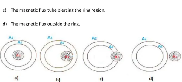
(10) To this aim, we calculate the energy spectra of different two-dimensional (2D) quantum rings pierced by different axial magnetic fields.. 3. ROLE OF SYSTEM TOPOLOGY ON THE AHARONOV BOHM EFFECT To study the role of the topology in the Aharonov Bohm effect, we calculate the energy spectrum of the system with the magnetic flux tube center located at different positions on the x-axis: a) The magnetic flux tube centered at the origin of coordinates b) The magnetic flux tube off-centered, but it is still within the inner hole of the ring. c) The magnetic flux tube piercing the ring region. d) The magnetic flux outside the ring.. Figure 4: Scheme of the systems with the magnetic flux tube at different locations along the x-axis. The continuous vector potential is defined in two separate regions A1 (non-zero magnetic field) and A2 (zero magnetic field).. The vector potential, as in the 1D quantum ring case, is defined in two regions: A1 corresponds to the region where the axial magnetic field is different from zero, and A2 corresponds to the zero magnetic field region. Moving the magnetic flux along the x-axis in the 2D system supposes an (x-x0) off centering:. Figure 5: The magnetic flux is displaced from the origin of coordinates to x0, along the x-axis.. A pedagogical approach to the Aharonov Bohm effect. Page 8.
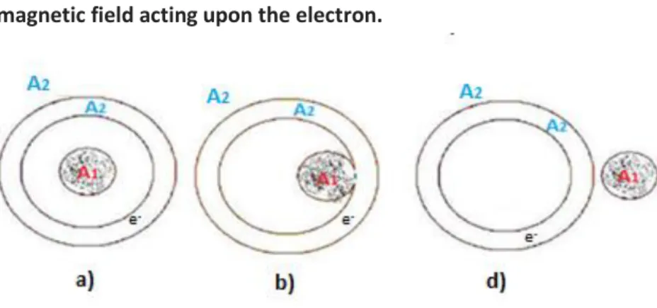
(11) As a consequence, the vector potential results: B0 (−y, (𝐱 − 𝐱𝟎 ),0) 2 B a2 = 20 R2 (−y, (𝐱 − 𝐱𝟎 ),0). 𝐀𝟏 (0 < R < a) =. A={ 𝐀𝟐 (a < R < ∞). ;. ∇ ∙ A = 0 (Coulomb gauge). (30). where a is the radius of the region pierced by the magnetic flux. As the magnetic is displaced from the origin of coordinates by x0, the radius R in the vector potential takes the form: R = √((𝒙 − 𝒙𝟎 )2 + y 2 ) (31) It should be noted that, while the magnetic field presents a discontinuity at R = a, the potential (30) is continuous A1(a)=A2(a). Next, we derive the Hamiltonian. The general expression for the Hamiltonian of an electron in the presence of a magnetic field, derived in a previous section (15), is: ћ2 2 iћ 𝑨𝒊 2 H=− 𝛻 − 𝑨𝒊 ∇ + 2m m 2m. (32). In a 2D space and Cartesian coordinates, the nabla operator has the form: 𝜕. 𝜕. 𝛻=(𝜕𝑥 + 𝜕𝑦). (33). By writing the nabla operator in its explicit form and using atomic units (ћ=1), we obtain the following Hamiltonian for an electron in the presence of a magnetic field in a 2D space: H=−. 1 𝜕 𝜕 2 i 𝜕 𝜕 𝐀𝒊 𝟐 ( + ) − 𝐀𝒊 ∙ ( , )+ 2m 𝜕𝑥 𝜕𝑦 m 𝜕𝑥 𝜕𝑦 2m. (34). The Hamiltonian is written in terms of Ai (i=1, 2) depending on the region where the magnetic field is zero or not.. 3.1 Zero magnetic field acting upon the electron.. Figure 6: The magnetic field acting upon the electron is zero. It occurs when the magnetic flux tube is completely inside the ring (cases a) and b)) or outside of it (case d)).. A pedagogical approach to the Aharonov Bohm effect. Page 9.
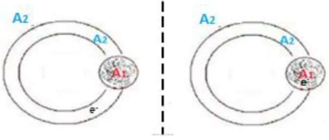
(12) The magnetic field acting upon the electron is zero in the cases when the magnetic flux tube is displaced but is still completely inside the quantum ring (cases a) and b)) or when it is outside of it (case d)) .Therefore, we must use the A2 component for the vector potential in the Hamiltonian: H=−. 1 𝜕 𝜕 2 i 𝜕 𝜕 𝐀𝟐 2 ( + ) − 𝐀𝟐 ∙ ( , )+ 2m 𝜕𝑥 𝜕𝑦 m 𝜕𝑥 𝜕𝑦 2m. (35). We inject the expression for A2, eq. (30), and find:. 1. 𝜕. 𝜕. 2. i 𝑩𝟎 𝒂𝟐 (−𝒚, (𝐱 𝟐 (𝒙−𝒙𝟎 )𝟐 +𝒚𝟐. H = − 2m (𝜕𝑥 + 𝜕𝑦) − 𝑚. 𝜕. − 𝐱𝟎 ), 𝟎) ∙ (𝜕𝑥 ,. 𝜕 ) 𝜕𝑦. 1 𝑩𝟎 𝟐 𝒂𝟒 𝟒 (𝒙−𝒙𝟎 )𝟐 +𝒚𝟐. + 2𝑚. (36). We can write the above equation in terms of the magnetic flux, which in atomic units reads: φ=. B0 πa2 (𝑎. 𝑢. ) (37) 2π. The resulting Hamiltonian is, then, a second order differential operator in terms of the magnetic flux:. H=−. 1 𝜕 𝜕 2 φ 1 𝜕 𝜕 𝜑2 1 ( + ) −i (−𝑦 + (𝑥 − 𝑥 ) ) + 0 2 2 2m 𝜕𝑥 𝜕𝑦 2m (𝑥 − 𝑥0 ) + 𝑦 𝜕𝑥 𝜕𝑦 2m (𝑥 − 𝑥0 )2 + y 2 (38). 3.2 Non-zero magnetic field acting upon the electron. Figure 7: The magnetic flux is piercing the electron density (case c)).. When the magnetic flux pierces the ring, then the electron crosses two regions where the potential vector is either defined as A2 or A1 (See figure 8). A magnetic field different from zero acts upon the electron in the region defined by A1, and a zero magnetic field acts upon it in the region defined by A2. A pedagogical approach to the Aharonov Bohm effect. Page 10.
(13) Figure 8: On the left, the electron passes by the region of the electron density of the ring, defined by A 2. On the right the electron passes by the region occupied by the magnetic flux, which is defined by the component A 1.. Therefore, now the Hamiltonian is different in each region. We employ the Hamiltonian previously derived for the region defined by A2, where the magnetic field is zero (38). Next, we derive it for the region of non-zero magnetic field, defined by A1. Then the general formula (34) takes now the form: H=−. 1 𝜕 𝜕 2 i 𝜕 𝜕 𝐀𝟏 𝟐 ( + ) − 𝐀𝟏 ∙ ( , )+ 2m 𝜕𝑥 𝜕𝑦 m 𝜕𝑥 𝜕𝑦 2m. (39). By inserting A1, eq. (30), we find: H=−. 1 𝜕 ( 2m 𝜕𝑥. +. 𝜕 2 ) 𝜕𝑦. −. i 𝑩𝟎 (−𝒚, (𝒙 − 𝑚 𝟐. 𝜕 𝜕𝑥. 𝒙𝟎 ), 𝟎) ∙ (. ,. 𝜕 1 𝑩𝟎 𝟐 )+ ((𝒙 − 𝜕𝑦 2𝑚 𝟒. 𝒙𝟎 )𝟐 + 𝒚𝟐 ) (40). This equation can also be written in terms of the magnetic flux:. 1 𝜕 𝜕 2 i 𝜕 𝜕 𝜑2 ((𝑥 − 𝑥0 )2 + 𝑦 2 ) (41) H=− ( + ) − 2 𝜑 (−𝑦 + (𝑥 − 𝑥0 ) ) + 2m 𝜕𝑥 𝜕𝑦 𝑎 m 𝜕𝑥 𝜕𝑦 2𝑚𝑎4. 4. SYMMETRY INFLUENCE ON THE AHARANOV BOHM EFFECT To study the interplay of symmetry and the Aharonov Bohm effect, the energy spectra of the following systems are calculated: -A circular ring -A hexagonal ring -A square ring In all cases, the magnetic flux is at the center of coordinates. The topology is the same for the three systems, only the symmetry of the system changes. The magnetic flux is inside the ring in the three systems, therefore the Hamiltonian obtained when the magnetic field acting upon the electron is zero is sufficient to study these systems.. A pedagogical approach to the Aharonov Bohm effect. Page 11.
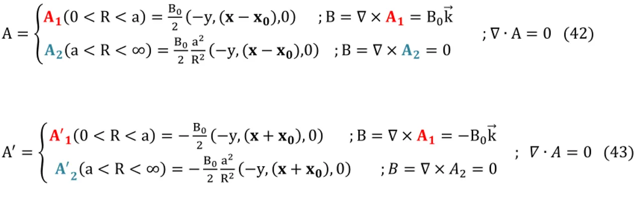
(14) 5. ROLE OF THE MAGNETIC FLUX ON THE AHARONOV BOHM EFFECT In order to assess the role of the magnetic flux in the Aharonov Bohm effect, we calculate the energy spectrum when there are two magnetic fluxes of opposed directions piercing the inner hole of a 2D quantum ring. Two variations of this case are explored: a) Two opposed fluxes are of equal magnitude b) One of the fluxes is twice the other (in absolute value).. 5.1 Opposite magnetic fluxes of equal magnitude. Figure 9: System with two opposed magnetic fluxes of equal magnitude, defined by vector potentials A and A’.. The total magnetic field is the sum of two opposite ones B and B’, each of them can be derived from the potential vector A and A’: B 𝐀𝟏 (0 < R < a) = 0 (−y, (𝐱 − 𝐱𝟎 ),0) ; B = ∇ × 𝐀𝟏 = B0 ⃗⃗ k 2 A={ 2 B a 𝐀𝟐 (a < R < ∞) = 0 2 (−y, (𝐱 − 𝐱𝟎 ),0) ; B = ∇ × 𝐀𝟐 = 0. ; ∇ ∙ A = 0 (42). 2 R. ′. A ={. B0 (−y, (𝐱 + 𝐱𝟎 ), 0) ;B 2 2 B a − 0 2 (−y, (𝐱 + 𝐱𝟎 ), 0) 2 R. 𝐀′ 𝟏 (0 < R < a) = − 𝐀′ 𝟐 (a < R < ∞) =. = ∇ × 𝐀𝟏 = −B0 ⃗⃗ k ; 𝐵 = ∇ × 𝐴2 = 0. ; 𝛻 ∙ 𝐴 = 0 (43). Then, the Hamiltonian for this system must include the total vector potential, sum of both potentials: H=. (p̂ + (𝐀𝟐 + 𝐀′𝟐 ))2 2m. (44). The components A2 and A’2 are used because the electron moves in the region where the magnetic field is zero. As in the previous cases, we write the Hamiltonian in terms of the magnetic flux (see details in Appendix 3): A pedagogical approach to the Aharonov Bohm effect. Page 12.
(15) 1 𝜕 𝜕 2 i 1 𝜕 𝜕 H=− ( + ) − 𝜑 (−𝑦 + (𝑥 − 𝑥0 ) ) 2m 𝜕𝑥 𝜕𝑦 m (𝑥 − 𝑥0 )2 + y 2 𝜕𝑥 𝜕𝑦 i 1 𝜕 𝜕 𝜑2 1 (𝑥 ) + 𝜑 (−𝑦 + + 𝑥 ) + 0 2 2 m (𝑥 − 𝑥0 ) + y 𝜕𝑥 𝜕𝑦 2m (𝑥 − 𝑥0 )2 + y 2 (𝑦 2 + 𝑥 2 − 𝑥0 2 ) 𝜑2 1 𝜑2 + − (45) 2m (𝑥 + 𝑥0 )2 + y 2 2m ((𝑥 − 𝑥0 )2 + y 2 )((𝑥 + 𝑥0 )2 + 𝑦 2 ). 5.2 Opposite magnetic fluxes of different magnitude. In this case, a magnetic field is twice and opposite to the other, so the vector potential must be: 𝐀𝟏 (0 < R < a) = B0 (−y, (𝐱 − 𝐱𝟎 ),0) ; B = ∇ × 𝐀𝟏 = 2B0 ⃗⃗ k 2 A={ a 𝐀𝟐 (a < R < ∞) = B0 2 (−y, (𝐱 − 𝐱𝟎 ),0) ; B = ∇ × 𝐀𝟐 = 0. ; ∇ ∙ A = 0 (46). R. ′. A ={. B0 (−y, (𝐱 + 𝐱𝟎 ), 0) ;B 2 2 B a − 0 2 (−y, (𝐱 + 𝐱𝟎 ), 0) 2 R. 𝐀′ 𝟏 (0 < R < a) = − 𝐀′ 𝟐 (a < R < ∞) =. ⃗⃗ = ∇ × 𝐀𝟏 = −B0 k ; 𝐵 = ∇ × 𝐴2 = 0. ; 𝛻∙𝐴 =0 (47). The obtained Hamiltonian is (See Appendix 3 and Appendix 4 for details):. 1 𝜕 𝜕 2 i 1 𝜕 𝜕 H=− ( + ) − 2𝜑 (−𝑦 + (𝑥 − 𝑥0 ) ) 2 2 (𝑥 ) 2m 𝜕𝑥 𝜕𝑦 m − 𝑥0 + y 𝜕𝑥 𝜕𝑦 i 1 𝜕 𝜕 2𝜑2 1 + 𝜑 (−𝑦 + (𝑥 + 𝑥0 ) ) + 2 2 m (𝑥 − 𝑥0 ) + y 𝜕𝑥 𝜕𝑦 2m (𝑥 − 𝑥0 )2 + y 2 (𝑦 2 + 𝑥 2 − 𝑥0 2 ) 𝜑2 1 2𝜑2 + − (48) 2m (𝑥 + 𝑥0 )2 + y 2 2m ((𝑥 − 𝑥0 )2 + y 2 )((𝑥 + 𝑥0 )2 + 𝑦 2 ). A pedagogical approach to the Aharonov Bohm effect. Page 13.
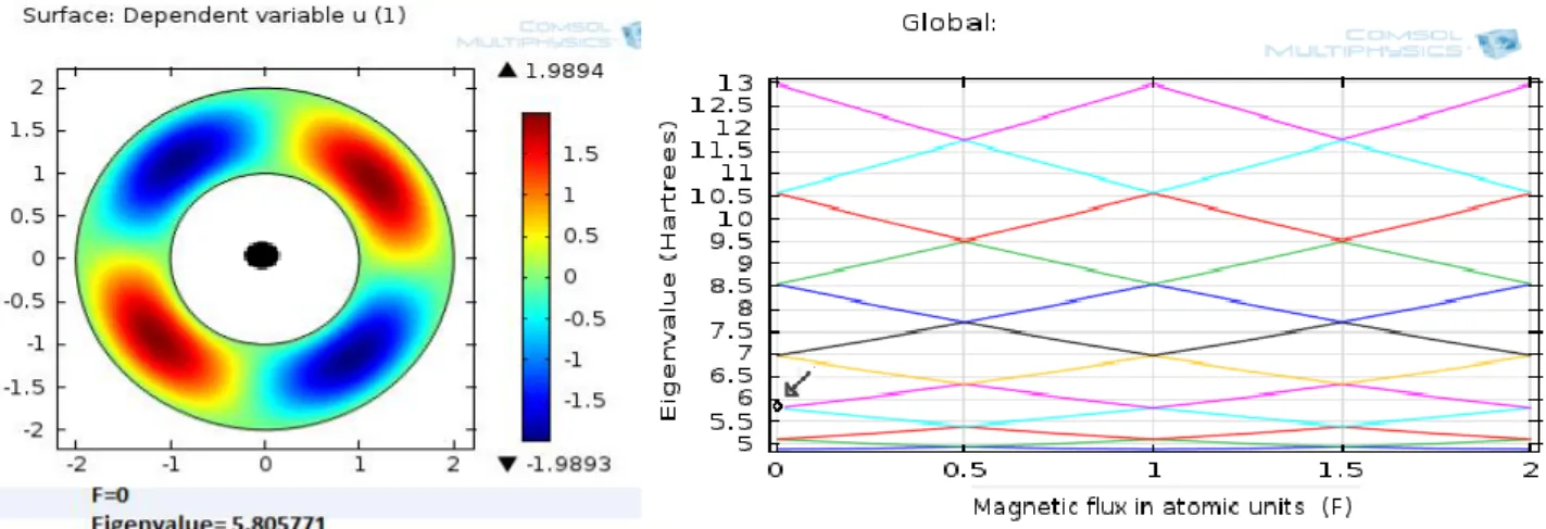
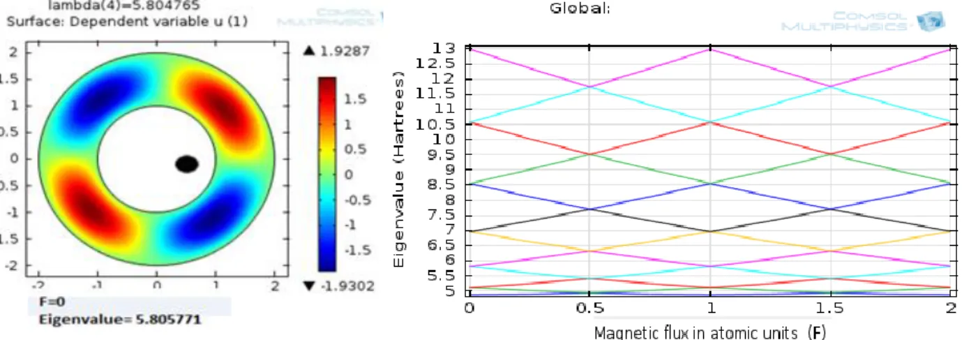
(16) 6. RESULTS The eigenvalue equations of the Hamiltonians obtained in previous sections are second order differential equations. We employ the Comsol multiphysics program package to obtain the energy levels and associated wave functions. We display the obtained results in the following sections.. Figure 10: Image of the employed program package: Comsol multiphysics.. 6.1 Aharonov Bohm effect: magnetic flux centered at the origin of coordinates First, we study the system for the case when the magnetic flux is centered at the origin of coordinates inside a 2-dimensional circular ring. We use atomic units to describe the system. The ring has an inner Bohr radius of 1 and an outer Bohr radius of 2, and the mass of the charged particle is the electron mass. We inject these parameters and the Hamiltonian of the system (38) into the Comsol program package and we obtain two different representations (see figure 11).. Figure 11: Representations obtained with the Comsol multiphysics program for a 2D-circular ring with the magnetic flux centered at the origin of coordinates. The effect of the magnetic flux (F) on the electronic wave function is represented on the left and the effect on the electronic eigenvalues (energy) on the right. The arrow in the energy spectrum points to the state corresponding to the wave function represented on the left. The black circle in the wave function representation represents the position of the magnetic flux.. The representation on the right (figure 11) shows the effect of the magnetic flux on the energy of the system. It shows the energy of the system (eigenvalues of the second order differential equation) versus the magnetic flux (F). Each line in the representation is an electronic state corresponding to a different value of the quantum magnetic number M. There is a total of 12 electronics states represented with the following respective values of M=0, ±1, ±2, ±3, ±4, ±5 and−6. We see how the energy of the electronic states is affected for different values of the magnetic flux situated in the center of coordinates. The range of values for the magnetic flux is from 0 to 2 atomic units. A pedagogical approach to the Aharonov Bohm effect. Page 14.
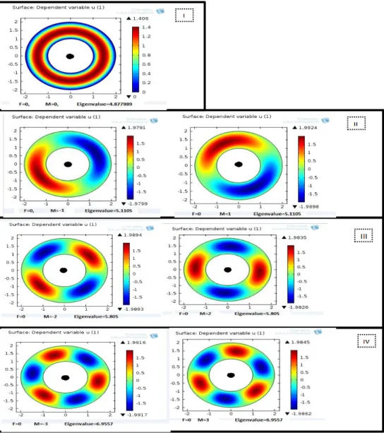
(17) We established, in the 1D-quantum ring example studied, that when the Aharanov Bohm effect takes place, the energy of the system depends, not only on the quantum magnetic number M, but also on the magnetic flux (29). This shows the presence of the Aharanov Bohm effect in the system. We see in the present case that the energy of the electronic states varies, increasing or decreasing, with the magnetic flux, so we can confirm the presence of the Aharonov Bohm effect. On the other hand, the representation on the left (figure 11) shows the effect of the magnetic flux on the wave function of the electron for a chosen value of the energy (Eigenvalue=5.805771) and of the magnetic flux (F=0). We can choose, for example, to represent the electronic wave function for the four lowest Eigenvalues when the magnetic flux is zero (F=0) (see figure 12):. Figure 12: Representations of the effect of the magnetic flux on the wave function of the electron for a fixed value of the magnetic flux, F=0. The states represented correspond to the four lowest electronic states with quantum numbers: M=0 (I), M=±𝟏 (II), M=±𝟐 (III) and M=±𝟑 (IV).. A pedagogical approach to the Aharonov Bohm effect. Page 15.
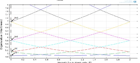
(18) The wave functions represented (figure 12) show that as the quantum number M increases, the number of nodes of the function increases and so the symmetry of the wave function changes from one Eigenstate to another. This difference in symmetry between electronics states coupled with the variation in energy due to the effect of the magnetic flux causes the crossing observed in the presence of the Aharonov Bohm effect. The electronic states represented in figure 12 with quantum number M equal in magnitude (M=±1, ±2, ±3) are degenerated for a null magnetic flux (F=0) as shown in figure 13.. Figure 13: The electronic states represented in figure 12 for a null magnetic flux (F=0) correspond to the following points in the energy spectrum.. This is because, in absence of magnetic flux (F=0), the energy of the system only depends on the quantum number M as shown in the 1D-ring toy example (see eq. 29) and the electronic states present degeneracy for values of M of equal magnitude (M=±1, M=±2,M=±3…) due to the symmetry of the system. However, we can see that the effect of the magnetic flux on the energy causes the states to lose their degeneracy and as consequence the crossing of the energy levels is produced. Now, we have seen the effect of the magnetic flux on the energy; but one may wonder ¿What is the effect of the magnetic flux on the wave function? To study the effect of the magnetic flux on the electron wave function we can represent the wave function of a determined electronic state for different values of the magnetic flux. The following figure (figure 14) shows the electronic state and the chosen values of the magnetic flux in the electronic energy spectrum.. A pedagogical approach to the Aharonov Bohm effect. Page 16.
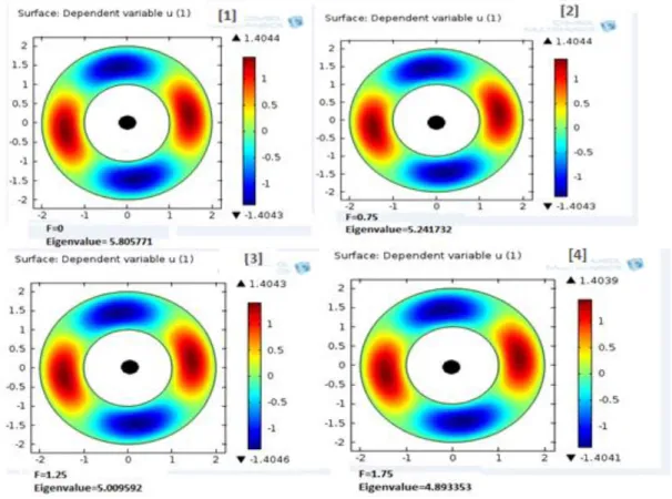
(19) Figure 14: The values of the magnetic flux chosen (F) for a determined energy level are: F=0 [1], F=0.75[2], F=1.25 [3] and F=1.75 [4]. The energy level corresponds to M=-2.. The points marked in figure 14 correspond to fixed values of the magnetic flux on the energy level chosen. As we have already seen, the energy associated to each of point is different due to the Aharonov Bohm effect. The electron wave function associated to those points is (see figure 15):. Figure 15: Representations of the wave function for the states indicated in figure 14.. The wave functions represented are identical; this means that the wave function of an electronic state remains the same independently of the value of the magnetic flux. It is only. A pedagogical approach to the Aharonov Bohm effect. Page 17.
(20) affected at the points of crossing of the energy levels where two different wave functions coincide. In summary, we see that the Aharonov Bohm effect causes the crossing of the energy levels due to the effect of the magnetic flux on the energy of the system and to the different symmetry of the electronic states. While on the other hand, the wave function for an energy level remains unaffected by the magnetic flux.. 6.2 Role of the system topology. To study the role of the topology of the system in the Aharonov Bohm effect we displace the system along the x axis and study the energy spectra for the following 3 cases. -Case 1: The magnetic flux is displaced from the origin of coordinates but is still restricted to the area inside the quantum ring. We study the system when the magnetic flux is displaced from the origin of coordinates but still is completely inside the ring. We have displaced it 0.2 Bohr radiuses from the origin of coordinates (results are in figure 16).. Figure 16: Representations obtained for the case when the magnetic flux (black circle in the representation) is displaced from the origin of coordinates but is still restricted to the area inside the quantum ring.. The representations show identical results to the ones obtained for the magnetic flux centered at the origin of coordinates (figure 11). We can confirm the presence of the Aharonov Bohm effect because of the crossing of the energy levels observed, which is consequence of the effect of the magnetic flux on the energy (representation at the right). In addition to it, the energy spectrum is identical in both systems. This is because the total magnetic flux is the same in both cases. We can therefore conclude that the system displays the Aharonov Bohm effect when the magnetic flux is completely in the region inside the ring. In that case, when the magnetic flux. A pedagogical approach to the Aharonov Bohm effect. Page 18.
(21) pierces the inside of the ring electron density, the systems present the same non-trivial topology, of doubly-connected space. -Case 2: The magnetic flux is piercing the electron density of the ring. Next, we study the system when the magnetic flux is piercing the electron density of the ring.. Figure 17: Representations for the case when the magnetic flux is piercing the electron density of the ring. The black circle in the wave function representation (left) represents the magnetic flux.. In this case, we see that when the magnetic flux pierces the ring electron density, the effect of the magnetic flux on the energy is weaker than in the previous cases (right representation) and as a consequence no more energy crossings occur. Now, the wave function is affected by the magnetic field (left representation), the system is affected by the field and, the effective flux piercing the ring hole is smaller. We see that when the system is in the “state of transition”, where the magnetic flux is not inside or outside the ring, but is piercing the electron density of the ring, the Aharonov Bohm effect is still partially present. Case 3: The magnetic flux is in the region outside the ring. Finally, we study the case where the magnetic flux is outside the ring. To do that we displace the magnetic flux 2.5 Bohr radiuses from the origin.. Figure 18: Representations obtained for the case when the magnetic flux is in the region outside the ring.. A pedagogical approach to the Aharonov Bohm effect. Page 19.
(22) When the magnetic flux is outside the ring, the system no longer displays the Aharonov Bohm effect, the electron is no longer affected by the magnetic flux and therefore no crossing of the energy levels is produced. The absence of the Aharonov-Bohm effect comes from the fact that when the magnetic flux is outside the ring then, it does not reveal the non-trivial topology of the system. If the Aharonov-Bohm effect does not take place, then the energy is not affected by the magnetic flux and it only depends on the quantum number M. Due to the symmetry of the system, the electronic states with the same quantum number M (M= ±1, ±2, ±3 …) are degenerate, as shown in the figure. Therefore, we confirm the relevance of the system topology on the presence or absence of the Aharonov-Bohm effect. We conclude that it is necessary that the magnetic flux pierces the inside of the electron density of the system for the Aharonov-Bohm effect to take place. That is to say, the topology of the system must be non-trivial (e.g. a doubly connected space).. -Case 4: An aperture is made on the quantum ring. Finally, we make an aperture on the ring to further see the role of the topology on the Aharonov Bohm effect. The aperture made is of 0.005 Bohr radiuses (figure 19).. Figure 19: Representations for a circular ring with an aperture in it. The magnetic flux is centered at the origin of coordinates. The system does not display the Aharonov Bohm effect. However the energy spectrum is different from the one obtained when the magnetic flux is outside the ring (figure 18).This is because the aperture made breaks the circular symmetry of the ring. We will now explain this result by looking to the wave functions. The probability of finding the particle in the region of the aperture is zero; therefore if the aperture is small enough we can consider it as a line that undoes the circle at angle values 0 = 2𝜋 and so the electronic wave function is defined by the following boundary conditions: 𝛹(0) = 𝛹(2𝜋) = 0 (49). A pedagogical approach to the Aharonov Bohm effect. Page 20.
(23) Then, the system is similar to that of a particle in a 2D box.. Figure 20: Illustration of the equivalence between a particle in ring with an aperture (left) and a particle in a box of length 2𝝅 (right). The aperture has an infinite potential for the electronic wave function in the same way the walls of the box have one.. A similar result is obtained by changing the symmetry of the system. In the case of a square or hexagonal ring, the results are:. Figure 21: Representations obtained for a square ring of inner length of 1 Bohr radius and outer length of 2 Bohr radiuses with an aperture in it. The magnetic flux is centered at the origin of coordinates. Figure 22: Representations obtained for a hexagonal ring with an inner side of 1 Bohr radius and an outer side of 2 Bohr radiuses, with an aperture in it. The magnetic flux is centered at the origin of coordinates. The Aharonov-Bohm is absent in all the cases, independently of the symmetry of the system. A pedagogical approach to the Aharonov Bohm effect. Page 21.
(24) This is because again the decisive factor is the topology of the system. In the three cases the system no longer has an interior and so the electron is no longer affected by the magnetic flux. The topology is trivial (simple connected space) and so the Aharonov Bohm effect does not take place. This result reiterates the importance of the topology in the absence/presence of the Aharonov Bohm effect. We see that it is necessary for the system to have an inside for the Aharonov Bohm effect to take place and that inside must be pierced by a magnetic flux.. 6.3 Symmetry influence We have seen the decisive role that the topology of the system plays in the presence or absence of the Aharonov-Bohm effect so that only systems with a certain topology (doubly connected space) display it. The next question that may arise from this is: ¿Does the symmetry of the system also affect the presence or absence of the Aharonov-Bohm effect in system? To answer this question, we have studied 3 systems with the same topology but different symmetry: a circular ring, a hexagonal ring and a square ring. All of them with the magnetic flux centered at the origin of coordinates.. a) Circular 2D-ring. Figure 23: Representations for a circular ring with the magnetic flux at the origin of coordinates.. The presence of the Aharonov-Bohm effect for a circular ring with the magnetic flux centered at the origin of coordinates has already been established in the previous section. However, now we will give a little insight into the effect of symmetry on the energy spectrum of the system. The symmetry of the system is 𝐶∞ due the presence of a magnetic field along the z-axis. This symmetry group has an infinite number of irreducible representations that can be labeled by an integer number m (see table): A pedagogical approach to the Aharonov Bohm effect. Page 22.
(25) Table 1: Symmetry table for the 𝑪∞ group.. As a result, the energy spectrum for the circular ring system presents an infinite number of energy states with different symmetry. We can see that it is the different symmetry of the electronic states coupled with the effect of the magnetic flux on the energy, characteristic of the Aharonov Bohm effect, what produces as a result the continuous crossing of the energy levels observed in the energy spectra of the system (figure 23).. b) Hexagonal ring. Figure 24: Representations for a hexagonal ring with the magnetic flux at the origin of coordinates. The hexagon ring presents an inner side of 1 Bohr radius and an outer side of 2 Bohr radiuses. The anti-crossing region and the electronic states with B symmetry, for which the anti-crossing occurs, have been signaled (right).. In the case of a hexagonal ring, we also confirm the presence of the Aharonov-Bohm effect because of the crossings observed due to the effect of the magnetic flux on the energy. However, now the energy spectrum also shows regions with anti-crossings. Those regions are repeated for every group of six electronic states in the energy spectrum (figure 24, right representation). This anti-crossing of the electronic states occurs because there is a symmetry reduction, from the 𝐶∞ group of the circular ring, with an infinite number of irreducible representations, to the 𝐶6 group of the hexagonal ring, with just 6 irreducible representations (see table) . A pedagogical approach to the Aharonov Bohm effect. Page 23.
(26) Table 2: Symmetry table for the C6 group.. So there are six different possible symmetry representations for the electronic states that are repeated along the energy spectrum of the hexagonal ring in contrast to the infinite number presented in the circular ring. We can see that, at the lowest energy, the configuration of electronic states for the hexagonal ring is:. Figure 25: Energy diagram showing the configuration of the electronic states for a hexagonal ring. The states for which anti-crossing takes place are indicated in it.. From lowest to highest energy, the first six electronic states are A, E1, E2 and B; then the anticrossing occurs; and the order of symmetry is reversed so the next six electronic states are B, E2, E1 and A. We see that the anti-crossing occurs for electronic states of the same symmetry, of B symmetry in this case. Due to the reduction in symmetry in going from the circle to the hexagon, energy states that were degenerated for the 𝐶∞ group are no longer degenerated for the 𝐶6 group. The following. A pedagogical approach to the Aharonov Bohm effect. Page 24.
(27) table, taken from a paper where this symmetry reduction is demonstrated [10], shows the equivalence between the representations when the symmetry is reduced from 𝐶∞ to 𝐶6 :. Table 3: Table that shows the equivalence between irreducible representations for a symmetry reduction, from a C∞ to a C6 group. Red rectangles are used to signal the representations that no longer are degenerated in the C6 group due to the reduction in symmetry. The table shows that electronic states which are degenerated in the 𝐶∞ group are no longer degenerated in the 𝐶6 group (states marked in red in table 3). For example, degenerated electronic states in the 𝐶∞ group with symmetry Гm=3 and Гm=-3, cease to be degenerated when in the 𝐶6 group, in which they both correspond to the same B symmetry. The same loss of degeneracy happens for the states with symmetry Гm=6 and Гm=-6 , where they correspond to the same A symmetry in the hexagonal ring. This is repeated all along the energy spectrum of the hexagonal ring for the equivalent states in the circle ring with symmetry: Гm=3 and Гm=-3, Гm=6 and Гm=-6, Гm=9 and Гm=-9 , … Therefore, the loss of degeneracy consequence of the reduction in symmetry is the reason for the anti-crossings observed in the hexagonal ring of states with the same symmetry.. A pedagogical approach to the Aharonov Bohm effect. Page 25.
(28) c) Square ring. Figure 26: Representations obtained for a square ring with the magnetic flux at the origin of coordinates. The square ring presents an inner length of 1 Bohr radius and an outer length of 2 Bohr radiuses. The anti-crossing regions are signaled in the energy spectrum (right).. We study a third case, a square ring, in order to further confirm the role of the symmetry in the Aharonov-Bohm effect. We see that the Aharonov-Bohm effect is also present for the square ring as in the circular and hexagonal ring cases. The energy spectrum also shows anti-crossings due to the reduction in symmetry. The symmetry of the system is C4, with 4 irreducible representations:. Table 4: Symmetry character table for the C4 group. Therefore, the energy spectrum of the systems presents 4 possible symmetries for the electronic states. At the lowest energy, the configuration of the electronic states is:. A pedagogical approach to the Aharonov Bohm effect. Page 26.
(29) Figure 27: Energy diagram that shows the configuration of the electronic states for a square ring. The anticrossing region is signaled in it.. Again, we see that the anti-crossing occurs for the states with the same symmetry, the B symmetry. And after the anti-crossing occurs, the order of symmetry for the electronic states is reversed. From lowest to highest energy, it starts with the symmetry A, E and B, then the anticrossing occurs, and the order in symmetry is reversed: B, E and A. This is repeated along the entire energy spectrum of the system. In conclusion, we see that the symmetry does not affect the presence or absence of the Aharonov-Bohm effect because the 3 systems studied display it independently of their symmetry. However it does affect the energy spectrum of the system causing the anti-crossing for energy states of the same symmetry.. 6.4 Role of the magnetic flux. Last but not least, we study the role of the magnetic flux in the Aharonov Bohm effect. To do that, we study the response of the system when the total magnetic flux piercing the electron density of the system is different. We study 2 cases: -When there are two magnetic fluxes inside the ring, of equal magnitude but opposing directions. -When there are two magnetic fluxes inside the ring of opposing directions, one of them being twice in magnitude the other.. A pedagogical approach to the Aharonov Bohm effect. Page 27.
(30) . There are two magnetic fluxes inside the ring, of equal magnitude but opposing directions.. Figure 28: Representations obtained when there are two magnetic fluxes (red and blue circles) inside the ring, of equal magnitude but opposing directions. The magnetic fluxes are each one at 0.5 Bohr radiuses from the origin of coordinates.. First we study the system when there are two magnetic fluxes inside the ring, of equal magnitude but opposing directions. We see that the response of the system is the same as if there was no magnetic flux at all. The reason for this is that the opposing magnetic fluxes cancel each other so the total magnetic flux piercing the electron density of the system is zero. We can see that the response of the system depends not on the individual fluxes but on the total magnetic flux piercing the electron density of the system.. . There are two magnetic fluxes inside the ring of opposing directions, one of them is twice in magnitude the other. Figure 29: Representations obtained for the case when there are two magnetic fluxes inside the ring of opposing directions, one of them is twice in magnitude the other.. Now, when one of the fluxes is twice in magnitude the other, the energy and wave function representations obtained are identical to the ones obtained for the cases of a circular ring with A pedagogical approach to the Aharonov Bohm effect. Page 28.
(31) a magnetic flux completely inside the ring (figures 16 and 11). The response of the system is the same as if there was one magnetic flux inside the ring with magnitude equal to the sum of the magnitudes of both fluxes. Therefore we can conclude that, in the Aharonov-Bohm effect, the response of the system depends upon the total magnetic flux piercing the electron density of the ring.. 7. CONCLUSIONS So, the conclusions reached can be summarized as: 1) The dynamics of a charged particle can be affected even if the magnetic field acting upon it is zero. This is what the Aharonov-Bohm effect predicts. 2) Simple-connected systems do not display this effect. 3) Double-connected systems display this effect when the magnetic field pierces the “inside” of the electronic density charge. 4) It is the total field flux piercing the system what matters. The response of the system depends on the total field flux piercing the electron density of the system. 5) Symmetry affects the energy spectra, causing the anti-crossing of same symmetry states, but it does not affect the presence/absence of the Aharonov-Bohm effect.. ACKNOWLEDGMENTS I want to thank my tutor Josep Planelles for his teachings and guidance during the realization of this work.. A pedagogical approach to the Aharonov Bohm effect. Page 29.
(32) 8. BIBLIOGRAPHY [1] Aharonov, Y., and Bohm, B., “Significance of Electromagnetic Potentials” in the Quantum Theory, Phys. Rev., 115, (1959) 485-491 [2] “An Elementary Primer for Gauge Theory” ,by K Moriyasu. World Scientific, 1983 (ISBN 9971950839, 9789971950835) [3] “Classical Mechanics”, by R. Douglas Gregory. Cambridge University Press, 13 April. 2006. Chapter Twelve: “Lagrange’s equations and conservation principles”, pp.pp.348-351. [4] J. Planelles, J.I. Climente and J.L. Movilla,"Aharonov-Bohm effect for pedestrian",in “Symmetry, Spectroscopy and SCHUR”, Proceedings of the Prof. Brian G. Wybourne Commemorative Meeting, Torun 12-14, June 2005, Eds.: R.C. King, M. Bylicki and J. Karwowski, N. Copernicus Univ. Press, Torun 2006, pp. pp.223-230 (ISBN 83-231-1901-5) [5]http://www3.uji.es/~planelle/APUNTS/QQ/AB.html [6] B. J. Hiley. "The Early History of the Aharonov-Bohm Effect". TPRU, Birkbeck. [7] A. Kregar (Mentor: prof. dr. A. Ramšak), “Aharonov-Bohm effect”, University of Ljubljana, Faculty of Mathematics and Physics, Department of physics, Seminar 4, Ljubljana, 2011. [8]Oliver Orasch (Supervisor: Ulrich Hohenester),” The Aharonov-Bohm-Effect”, University of Graz, Bachelor Thesis, December 16, 2014. [9] Aharonov-Bohm Effect. "Quantum Effects on Charged Particles in Field-Free Regions". American Journal of Physics 38, 162 (1970) [10] A. Ballester, C. Segarra, A. Bertoni and J. Planelles. "Suppression of the Aharonov-Bohm effect in six-electron hexagonal quantum rings" Eur. Phys. Lett., 104 (2013) 67004.1-6.. A pedagogical approach to the Aharonov Bohm effect. Page 30.
(33) 9. APPENDIX. A pedagogical approach to the Aharonov Bohm effect. Page 31.
(34) Appendix 1 Hamiltonian for a charged particle in the presence of a magnetic field.. In this appendix, first we show how for conservative systems, Newton’s equation can be derived from the Lagrange equation. Then we introduce the Lagrangian for a charged particle in the presence of a magnetic field and proof it by deriving the Lorenz force from it. Finally, we derive the Hamiltonian from the Lagrangian introduced.. . LANGRAGIAN FOR A CONSERVATIVE SYSTEM. In conservative systems, the potential (V) only depends on spatial coordinates: 𝑉 = 𝑉(𝑞) (50) Where q refers to generalized coordinates. Therefore the corresponding force (F) also depends on the spatial coordinates. 𝐹=−. 𝑑𝐹 𝑑𝑉. ; 𝐹(𝑞) (51). The force according to Newton’s second law is: 𝐹 = 𝑚𝑎 (52) Which can also be written in terms of the linear momentum (p=mv) in the form: 𝑑𝑝 −𝐹 =0 𝑑𝑡. (53). We will show that Newton’s law equation (53) is equivalent to the following equation for conservative systems: 𝑑 𝜕𝐿 𝜕𝐿 ( )− = 0 (1 ≤ 𝑖 ≤ 𝑛) (54) 𝑑𝑡 𝜕𝑞̇ 𝑖 𝜕𝑞𝑖 This is the Lagrange’s equation for a conservative system where L is called the Lagrangian of the system and is written as the Kinetic energy (T) minus the potential (V). The Lagrangian for a conservative system where the potential V depends only on the spatial coordinates is: 1 𝐿 = 𝑚𝑞̇ 2 − 𝑉(𝑞) 2. A pedagogical approach to the Aharonov Bohm effect. (55). Page 32.
(35) Then:. 𝜕𝐿 = 𝑚𝑞𝑖̇ = 𝑝𝑖 (56) 𝜕𝑞̇ 𝑖. 𝜕𝐿 𝜕𝑉 =− = 𝐹𝑖 𝜕𝑞𝑖 𝜕𝑞𝑖. (57). We inject the results obtained (56 and 57) into equation (54) and obtain: 𝑑 (𝑝 ) − 𝐹𝑖 = 0 𝑑𝑡 𝑖. (1 ≤ 𝑖 ≤ 𝑛) (58). Thus we proof that Langrage’s equation takes the form of Newton’s second law equation for conservative systems.. . LANGRAGIAN FOR A FOR A CHARGED PARTICULE IN A STATIC MAGNETIC FIELD :VELOCITY DEPENDENT POTENTIALS. Suppose a charged particle moving in the x-direction, when a magnetic field is acting upon it, the resultant Lorenz force (60) is perpendicular to the velocity of the particle and to the magnetic field. As a consequence the particle moves in a circular motion:. ⃗⃗) (59) 𝐹⃗ = 𝑒(𝑣 × 𝐵. Figure 30: Circular motion of a charged particle when a magnetic field is acting upon it.. As a result, the force depends on the radius described and the velocity of the particle 𝐹(𝑟, 𝑣). Therefore the potential is velocity dependent. Nonetheless, we can still write the equation of motion in Lagrangian form. First, we will introduce the Lagrangian for the system and then proof it by deriving the Lorenz force from it. The Lagrangian for a charged particle now presents a velocity dependent potential (term in bold in eq. 60): A pedagogical approach to the Aharonov Bohm effect. Page 33.
(36) 1 𝐿 = 𝑚𝑞̇ 2 + 𝒆𝒒̇ ∙ 𝑨(𝒒) (60) 2 Where e is charge of the particle and A is the vector potential that defines the magnetic field acting on the particle. We take the generalized coordinates to be the Cartesian coordinates (x,y,z) of the particle: 𝑞 = (𝑞𝑥 , 𝑞𝑦 , 𝑞𝑧 ) = (𝑥, 𝑦, 𝑧) (61) So the potential is: 𝐴 = (𝐴𝑥 , 𝐴𝑦 , 𝐴𝑧 ). (62). The Lagrange equation for the motion of the particle along the x axis has the form: 𝑑 𝜕𝐿 𝜕𝐿 ( )− = 0 (63) 𝑑𝑡 𝜕𝑥̇ 𝜕𝑥 We take into account that the spatial coordinates may depend on time even though A does not directly depend on time and proceed to derivate: 𝜕𝐿 = 𝑚𝑥̇ + 𝑒𝐴𝑥 (64) 𝜕𝑥̇ 𝜕𝐿 𝜕𝐴𝑖 =𝑒 ∑ 𝑞̇ 𝜕𝑥 𝜕𝑥 𝑖. (65). 𝑖=𝑥,𝑦,𝑧. We replace equations (64 and 65) into the Lagrange equation (63): 𝑑 𝜕𝐴𝑖 (𝑚𝑥̇ + 𝑒𝐴𝑥 ) − 𝑒 ∑ 𝑞̇ = 0 𝑑𝑡 𝜕𝑥 𝑖. (66). 𝑖=𝑥,𝑦,𝑧. The time derivative of the first term is: 𝑑 𝜕𝑥̇ 𝜕𝐴𝑥 (𝑚𝑥̇ + 𝑒𝐴𝑥 ) = 𝑚 + 𝑒 ∑ 𝑞̇ 𝑑𝑡 𝜕𝑡 𝜕𝑞𝑖 𝑖. (67). 𝑖=𝑥,𝑦,𝑧. So the resultant Lagrange equation is: 𝑚. 𝜕𝑥̇ 𝜕𝐴𝑥 𝜕𝐴𝑖 + 𝑒 ∑ 𝑞̇ 𝑖 − 𝑒 ∑ 𝑞̇ = 0 𝜕𝑡 𝜕𝑞𝑖 𝜕𝑥 𝑖 𝑖=𝑥,𝑦,𝑧. (68). 𝑖=𝑥,𝑦,𝑧. This can also be written as: 𝑚. 𝜕𝑥̇ 𝜕𝐴𝑖 𝜕𝐴𝑥 = 𝑒 ∑ 𝑞̇ 𝑖 ( − ) 𝜕𝑡 𝜕𝑥 𝜕𝑞𝑖. (69). 𝑖=𝑥,𝑦,𝑧. A pedagogical approach to the Aharonov Bohm effect. Page 34.
(37) If the summation term is expanded we obtain:. 𝑚. 𝝏𝑨𝒚 𝝏𝑨𝒙 𝜕𝑥̇ 𝜕𝐴𝑥 𝜕𝐴𝑥 𝝏𝑨𝒛 𝝏𝑨𝒙 = 𝑒 [𝑥̇ ( − ) + 𝑦̇ ( − − )] ) + 𝑧̇ ( 𝜕𝑡 𝜕𝑥 𝜕𝑥 𝝏𝒙 𝝏𝒚 𝝏𝒙 𝝏𝒛. (70). The first term in the brackets is zero and the other two written in bold are the magnetic field along the z axis (𝐵𝑧 ) and along the y axis (𝐵𝑦 ) respectively: 𝑚. 𝜕𝑥̇ = 𝑒[𝑦̇ (𝑩𝒛 ) + 𝑧̇ (𝑩𝒚 )] 𝜕𝑡. (71). The term in the brackets is the x component of the curl of the velocity with the magnetic field: 𝑚. 𝜕𝑥̇ = 𝑒(𝑞̇ × 𝐵)𝑥 𝜕𝑡. (72). Therefore we proof that the Lagrange introduced takes the form of the x component of the Lorenz force for a particle moving in the presence of a static magnetic field along the x axis: 𝑚. 𝜕𝑥̇ = 𝑒(𝑞̇ × 𝐵)𝑥 𝜕𝑡. 𝐹 = 𝑒(𝑞̇ × 𝐵)𝑥. (73) (74). The other components (y and z) can be obtained with the same procedure. For further reading see the book “Classical Mechanics”, by R. Douglas Gregory [3].. . HAMILTONIAN FOR A PARTICLE IN THE PRESENCE OF A MAGNETIC FIELD. An alternative formulation of classical mechanics to the Lagrangian relies on the Hamiltonian function. Both functions keep the same physical information but, while the Lagrangian depends on coordinate and velocity 𝐿(𝑞, 𝑞̇ ), the Hamiltonian depends on coordinate and momentum 𝐻(𝑞, 𝑝). This is similar to the different potentials used in thermodynamics to represent the state of a system: internal energy U(S, V), enthalpy H(S, P), Helmholtz free energy F (T, V), and Gibbs free energy G (T, P).All of them have the same information but depend on different coordinates (Temperature (T), Entropy (S), Pressure (P) and/or Volume (V). We can obtain, for example, the enthalpy H(S, P) from the internal energy U(S, V) by means of the following Lagrange transformation: 𝜕𝑈 𝐻(𝑆, 𝑃) = 𝑈 − 𝑉 ( ) 𝜕𝑉 𝑆. A pedagogical approach to the Aharonov Bohm effect. (75). Page 35.
(38) The Hamiltonian can be obtained from the Lagrangian in a similar way: −𝐻(𝑝, 𝑞) = 𝐿 − 𝑞̇ (. 𝜕𝐿 ) 𝜕𝑞̇. (76). −𝐻(𝑝, 𝑞) = 𝐿 − 𝑞̇ 𝑝 (77) Note that there is a change of sign so that H can be related to the energy. However the basis for the procedure is the same as the one used to obtain the thermodynamics potentials. In general, the Hamiltonian takes the following form for general coordinates: 𝐻 = ∑ 𝑝𝑖 𝑞̇ 𝑖 − 𝐿. (78). 𝑖=𝑥,𝑦,𝑧. But, before continuing with the Hamiltonian it is necessary to distinguish between the kinetic momentum (𝜋) , derived from the Kinetic energy, and the canonical momentum (p) which is derived from the Lagrangian: 𝜋𝑖 =. 𝜕𝑇 𝜕𝑞̇ 𝑖. (79). 𝑝𝑖 =. 𝜕𝐿 𝜕𝑞𝑖̇. (80). Both momentums (79 and 80) are the same for conservative systems in which the potential depends only on the space coordinates. However they are not for systems with velocity dependent potential such as the case studied in which: 𝜋𝑖 = 𝑝𝑖 =. 𝜕𝑇 = 𝑚𝑞̇ 𝑖 𝜕𝑞𝑖̇. (81). 𝜕𝐿 = 𝜋𝑖 + 𝑒𝐴𝑖 (82) 𝜕𝑞̇. We inject the equation obtained (82) into the expression for the Hamiltonian (78): 𝐻 = ∑ 𝑝𝑖 𝑞̇ 𝑖 − 𝐿 = ∑ (𝜋𝑖 + 𝑒𝐴𝑖 )𝑞̇ 𝑖 − 𝐿 (83) 𝑖=𝑥,𝑦,𝑧. 𝑖=𝑥,𝑦,𝑧. But the Lagrangian (L) in eq. (83) can also be written in terms of the kinetic momentum (81) as: 1 𝐿 = 𝜋𝑖 𝑞̇ 𝑖 + 𝑒𝑞̇ 𝑖 𝐴𝑖 (84) 2. We replace this expression for the Lagrangian in eq. (83): A pedagogical approach to the Aharonov Bohm effect. Page 36.
(39) 1 𝐻 = ∑ (𝜋𝑖 + 𝑒𝐴𝑖 )𝑞̇ 𝑖 − ∑ ( 𝜋𝑖 𝑞̇ 𝑖 + 𝑒𝑞̇ 𝑖 𝐴𝑖 ) 2 𝑖=𝑥,𝑦,𝑧. (85). 𝑖=𝑥,𝑦,𝑧. 𝐻= ∑ 𝑖=𝑥,𝑦,𝑧. 1 𝜋2 𝜋𝑖 𝑞̇ 𝑖 = (86) 2 2𝑚. Finally, we write the canonical momentum in its explicit form (82) in the equation (86), obtaining the Hamiltonian for a charged particle in a magnetic field: 𝐻=. 1 (𝑝 − 𝑒𝐴)2 (87) 2𝑚. A pedagogical approach to the Aharonov Bohm effect. Page 37.
(40) Appendix 2 Wave function for a particle in a 1D-ring In quantum mechanics, the case of a particle in a one-dimensional ring is similar to the particle in a box. The Schrödinger equation for a free particle which is restricted to a ring is: ћ2 2 ∇ 𝛹 = 𝐸𝛹 (88) 2𝑚. −. Where m is the mass of the particle and ∇2 , the Laplacian operator. Now, because the symmetry of the system is cylindrical the Laplacian operator can be written in polar coordinates (ρ,ϕ,z).However for a 1-dimensional ring, the wave function depends only on the angular coordinate, so: ∇2 =. 1 𝜕2 𝑅 2 𝜕𝜃 2. (89). Where R is the radius described by the particle and 𝜃, the angular coordinate. The Schrödinger equation is therefore: −. ћ2 𝜕 2 𝛹 = 𝐸𝛹 (90) 2𝑚𝑅 2 𝜕𝜃 2. It can also be written as: −. 𝜕2 2IE 𝛹 = 2 𝛹 (91) 2 𝜕𝜃 ћ. Where I = mR2 is the moment of inertia.. The equation obtained is of the form: −. 𝜕2 𝛹 = 𝑚2 𝛹 𝜕𝜃 2. (92). Where m is a constant defined as: 𝑚2 =. 2𝐼𝐸 ћ2. (93). The possible solutions to it are of exponential form:. 𝛹(𝜃) = 𝑁𝑒 ±𝑖𝑚𝜃. (94). Where N is the normalization constant. A pedagogical approach to the Aharonov Bohm effect. Page 38.
(41) A physically acceptable wave function must be single-valued. Since ϕ increased by any multiple of 2π represents the same point on the ring, then: 𝛹(𝜃 + 2𝜋) = 𝛹(𝜃) (95). Therefore: 𝑒 𝑖𝑚(𝜃+2𝜋) = 𝑒 𝑖𝑚𝜃. (96). This means that: 𝑒 𝑖2𝜋𝑚 = 1 (97) Which is only true is m is an integer: 𝑚 = 0, ±1, ±2, ±3 …. (98). The normalized wave function is: 𝛹𝑚 (𝜃) =. 1 √2𝜋. 𝑒 𝑖𝑚𝜃. A pedagogical approach to the Aharonov Bohm effect. (99). Page 39.
(42) Appendix 3 Two magnetic fluxes of equal magnitude and opposite directions: Derivation of the Hamiltonian operator.. Figure 31: Quantum ring with two magnetic fluxes inside of equal magnitude and opposite directions. One magnetic flux is defined by a potential A and the other, by A’.. The system presents now two magnetic fluxes so there are two potentials, A and A’, each one defining a magnetic field: 𝐵 =∇×𝐴. (100). 𝐵′ = ∇ × 𝐴′ (101) Therefore the total magnetic flux is the sum of both magnetic fields: 𝐵𝑡𝑜𝑡 = 𝐵 + 𝐵′ = ∇ × 𝐴 + ∇ × 𝐴′ = ∇ × (𝐴 + 𝐴′ ) (102) So first, it is necessary to define the potentials. Because the magnetic fluxes are of equal magnitude but opposing directions, A and A’ will present the same form, but with different signs, one will be positive while the other will be negative. The potentials, A and A’, can be defined as: B0 (−y, (𝐱 − 𝐱𝟎 ),0) 2 A={ B0 a2 (−y, (𝐱 − 𝐱𝟎 ),0) 𝐀𝟐 (a < R < ∞) = 2 R2 𝐀𝟏 (0 < R < a) =. (103). B0 (−y, (𝐱 + 𝐱𝟎 ), 0) 2 A′ = { B0 a2 (−y, (𝐱 + 𝐱𝟎 ), 0) 𝐀′ 𝟐 (a < R < ∞) = − 2 R2 𝐀′ 𝟏 (0 < R < a) = −. (104). where “a” is the radius of the area occupied by each magnetic flux and R is the radius. In the case of the potential A, R has the form: R = √((𝒙 − 𝒙𝟎 )2 + y 2 ) A pedagogical approach to the Aharonov Bohm effect. (105) Page 40.
(43) while for A’ it reads: R = √((𝒙 + 𝒙𝟎 )2 + y 2 ). (106). Each magnetic flux produces a magnetic field inside the ring different from zero along the zaxis. Then, we must define the components of the vector potential A1 and A’1 so that: B = ∇ × 𝐀𝟏 = B0 ⃗⃗ k (107) ⃗⃗ B = ∇ × 𝐀′𝟏 = −B0 k. (108). On the other hand, in the region of the electron density of the ring and outside it, the magnetic field is zero. Therefore, we must define A2 and A’2 in such a way that: B = ∇ × 𝐀𝟐 = 0. (109). B = ∇ × 𝐀′𝟐 = 0. (110). In addition, we can choose the Coulomb gauge for both potentials: 𝛻∙𝐴 =0. (111). 𝛻 ∙ 𝐴′ = 0. (112). The Hamiltonian for this system includes both potentials: H=. (p̂ + (𝑨𝟐 + 𝑨′𝟐 ))2 2m. (113). Where we use the components A2 and A’2 because the electron moves in the region where the magnetic field is zero.. Next, we expand the square binomial and apply the Coulomb gauge so that the linear momentum operator and the vector potentials commute, thus obtaining: 𝐻=. 𝑝̂ 2 (𝑨𝟐 + 𝑨′𝟐 )𝑝̂ (𝑨𝟐 + 𝑨′𝟐 )2 + + 2𝑚 𝑚 2𝑚. (114). We substitute the expressions for A2 (103) and A’2 (104) into the Hamiltonian and write the linear momentum in its explicit form: A pedagogical approach to the Aharonov Bohm effect. Page 41.
(44) 𝑝̂ = −𝑖ћ∇ ;. 𝜕 𝜕𝑥. 𝛻=(. +. 𝜕 ) 𝜕𝑦. (115). The obtained Hamiltonian is: 1 𝜕 𝜕 2 𝑖 𝑩𝟎 𝒂𝟐 𝜕 𝜕 𝐻=− ( + ) − (−𝒚 + (𝒙 − 𝒙𝟎 ) ) 𝟐 𝟐 2𝑚 𝜕𝑥 𝜕𝑦 𝑚 𝟐 (𝒙 − 𝒙𝟎 ) + 𝒚 𝜕𝑥 𝜕𝑦 𝟐 𝑖 𝑩𝟎 𝒂 𝜕 𝜕 𝐵0 2 𝑎4 (𝒙 ) + (−𝒚 + + 𝒙 ) + 𝟎 𝑚 𝟐 (𝒙 + 𝒙𝟎 )𝟐 + 𝒚𝟐 𝜕𝑥 𝜕𝑦 8𝑚 ((𝒙 − 𝒙𝟎 )2 + 𝑦 2 )2 2 2 4 4 (𝑦 2 2 𝐵0 𝑎 𝐵0 𝑎 + 𝑥 − 𝑥0 2 ) + − (116) 8𝑚 ((𝒙 + 𝒙𝟎 )2 + 𝑦 2 )2 4𝑚 ((𝑥 − 𝑥0 )2 + 𝑦 2 )((𝑥 + 𝑥0 )2 + 𝑦 2 ). where we show in blue the explicit forms of A2 and A’2. The last three terms correspond to the expanded square of the sum of both components. We can also write equation (116) in terms of the magnetic flux φ =. Bπa2 2π. (a.u.):. 1 𝜕 𝜕 2 i 1 𝜕 𝜕 H=− ( + ) − 𝜑 (−𝑦 + (𝑥 − 𝑥0 ) ) 2 2 2m 𝜕𝑥 𝜕𝑦 m (𝑥 − 𝑥0 ) + y 𝜕𝑥 𝜕𝑦 i 1 𝜕 𝜕 𝜑2 1 + 𝜑 (−𝑦 + (𝑥 + 𝑥0 ) ) + 2 2 m (𝑥 + 𝑥0 ) + y 𝜕𝑥 𝜕𝑦 2m (𝑥 − 𝑥0 )2 + y 2 (𝑦 2 + 𝑥 2 − 𝑥0 2 ) 𝜑2 1 𝜑2 + − (117) 2m (𝑥 + 𝑥0 )2 + y 2 2m ((𝑥 − 𝑥0 )2 + y 2 )((𝑥 + 𝑥0 )2 + 𝑦 2 ). A pedagogical approach to the Aharonov Bohm effect. Page 42.
(45) Appendix 4 Two magnetic fluxes of different magnitude and opposite directions: Derivation of the Hamiltonian operator.. Figure 32: Quantum ring with two magnetic fluxes inside of different magnitude and opposite directions.. We develop here the case of one of the fluxes being twice the other. It is similar to the problem studied in Appendix 3 with the only difference that the magnetic field defined by one vector potential is twice in magnitude the other.Therefore the potentials take the form: 𝐀𝟏 (0 < R < a) = B0 (−y, (𝐱 − 𝐱𝟎 ),0) ; B = ∇ × 𝐀𝟏 = 2B0 ⃗⃗ k A={ a2 𝐀𝟐 (a < R < ∞) = B0 R2 (−y, (𝐱 − 𝐱𝟎 ),0) ; B = ∇ × 𝐀𝟐 = 0. ′. A ={. B0 (−y, (𝐱 + 𝐱𝟎 ), 0) ;B 2 2 B a − 20 R2 (−y, (𝐱 + 𝐱𝟎 ), 0). 𝐀′ 𝟏 (0 < R < a) = − 𝐀′ 𝟐 (a < R < ∞) =. ;∇ ∙ A = 0. = ∇ × 𝐀𝟏 = −B0 ⃗⃗ k ; 𝐵 = ∇ × 𝑨𝟐 = 0. (118). ; 𝛻∙𝐴=0 (119). The procedure to obtain the Hamiltonian is also identical to that in Appendix 3 and the resulting Hamiltonian, in terms of the magnetic flux, finally reads: H=−. 1 𝜕 𝜕 2 i 1 𝜕 𝜕 ( + ) − 2𝜑 (−𝑦 + (𝑥 − 𝑥0 ) ) 2 2 (𝑥 − 𝑥0 ) + y 2m 𝜕𝑥 𝜕𝑦 m 𝜕𝑥 𝜕𝑦 i 1 𝜕 𝜕 2𝜑2 1 (𝑥 ) + 𝜑 (−𝑦 + + 𝑥 ) + 0 2 2 (𝑥 ) ((𝑥 m + 𝑥0 + y 𝜕𝑥 𝜕𝑦 2m − 𝑥0 )2 + y 2 ) 2 2 2 2 2 (𝑦 + 𝑥 − 𝑥0 ) 𝜑 1 2𝜑 + − (120) 2 2 2m (𝑥 + 𝑥0 ) + y 2m ((𝑥 − 𝑥0 )2 + y 2 )((𝑥 + 𝑥0 )2 + 𝑦 2 ). A pedagogical approach to the Aharonov Bohm effect. Page 43.
(46)
Figure
+7
Documento similar