TítuloFractional order identification based on time domain methodology for hydraulic canal system

Texto completo

(1)Actas de las XXXIX Jornadas de Automática, Badajoz, 5-7 de Septiembre de 2018 https://doi.org/10.17979/spudc.9788497497565.0688. Fractional-Order Identification Based On Time Domain Methodology For Hydraulic Canal System Gharab Saddam 1. Vicente Feliu-Batlle 1. [email protected] 1 2. Juan Carlos Cambera 1,2. [email protected]. [email protected]. Escuela Tecnica Superior de Ingenieros Industriales Ciudad Real, Spain. Instituto de Investigaciones Energeticas y Aplicaciones Industriales Ciudad Real, Spain. Abstract. an efficient tool that models more precisely some physical engineering processes, and accordingly it. This paper discusses the identification of hydraulic. was used as a promissory tool in bioengineering. canal system with a fractional-order model. The. [11], electronics [1], viscoelasticity [5], robotics [6,. identification procedure is carried out by using a. 7], control theory [2, 4], and signal processing [12,. time domain technique. A pseudorandom binary. 19] and others.. signal (PRBS) is considered, the auto-correlation. Thereafter, system identification using fractional. of the input signal, as well as, the impulsive re-. order models still represents a complicated task. sponse of the system has been concluded, and the. in comparison with classical identification. In the. obtained model are discussed in order to show the. case of classical integer systems, once the order. effect of using the PRBS signal in comparison with. of the system to be identified is selected, the pa-. a fundamental step signal. Finally, we put the ac-. rameters of the model can be optimized directly.. cent into the improvisation of the fractional-order. Although, for fractional-order systems, identifica-. model of the considered prototype that has a signifi-. tion procedure requires the choice of the number. cant impact on improving the performance of canal. of fractional operators and the fractional power of. monitoring, control, and supervisory systems. Keywords: order. these operators [14].. Fractional-order model, fractional-. identification,. PRBS,. Hydraulic. Thus, the identification process is significantly. canal. complicated each time the integer order is lost.. system.. Previous work in this area has been limited [3, 8, 18].. The authors in the before mentioned. works identify mechanical damping behavior and. 1. an electrode-electrolyte polarization for specifi-. INTRODUCTION. cally chosen transfer function forms and by usAlthough its application has shown interest only. ing frequency domain techniques. Fractional or-. in recent years, the theory of fractional-order cal-. der differential equations are more adequate than. culus has quite a long and prominent history. It. integer-order equations on modelling diffusion sys-. has defined as the generalization of classical cal-. tems as occurs in electrochemical processes [16,. culus to orders of integration and differentiation. 17].. not necessarily integer, and it has represented a. Works published in [13, 15] shown that there is. matter of almost exclusive interest for few mathe-. great potential for the use of fractional-order mod-. maticians and theoretical physicists.. els in depicting the dynamic behavior of irriga-. The complexity of such calculus, the evident self-. tion main canal pools. According to the same ref-. sufficiency of the integer order calculus, and the. erences, fractional-order models could accurately. fact that it does not have a fully acceptable geomet-. represent the dynamic model of hydraulic canal. rical or physical interpretation are the reasons of. systems, which has a significant impact on improv-. not being widely used in engineering sciences [10].. ing the performance of canal monitoring, control,. During the last decades, it has been presented as. and supervisory systems.. 688.

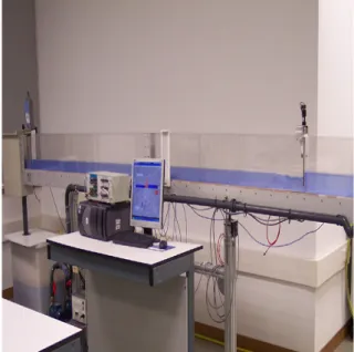
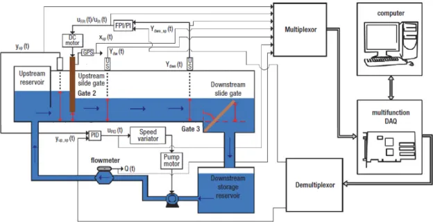
(2) In this work, fractional-order model for hydraulic. prototype is presented in Figure 1, and another. canal system is calculated using a new identifi-. schematic representation is depicted in Figure 2.. cation technique based on time domain data. A. The geometry of the downstream overshot gate is. new model has been explained, for the considered. shown on the left-hand side of Figure 2. The angu-. system, in order to enhance the precision of the. lar position of this gate can be manually adjusted. obtained results. The identification procedure is. to three values which yield gate top heights of 13,. based on PRBS signal which has been generated in. 23 and 33 mm above the canal bottom respectively.. function of the parameter of the system. The impulsive response of the system is calculated from the cross-correlation function of the resulting signals, and the fractional-order transfer function is concluded using the Laplace transform. The paper is organized as follows, the second Section represents a small definition of the considered system, Section 3 represents the new model of the considered SISO system, In Section 4, a comparison between the models obtained using the PRBS signal as an input on time domain identification and the classical identification based on step input signal is developed, and finally, Sections 5 represents some conclusions.. 2 THE HYDRAULIC CANAL. Figure 1: Prototype hydraulic canal in laboratory. PROTOTYPE 3 Time domain Identification. As it was mentioned in the introduction, the considered system is a closed-loop water variable slope. 3.1. rectangular canal characterized by glass walls and. Fractional-order model for the hydraulic canal prototype. a methacrylate bottom and located in the Fluids Mechanics Laboratory in the University Castilla-. The dynamics of the hydraulic canal are described. La Mancha (Spain). The description of the canal is. by the Saint-Venant equations, which are nonlin-. like 5 m of length, 8 cm of wide, and 25 cm high. ear hyperbolic partial differential equations [8].. for the walls. The platform of the prototype inte-. Linearized models around some flow regimes are. grates electromechanical sensors and actuators, a. often used in order to design canal controllers.. PLC (programmable logic controller) and a SCADA. The parameters of these approximated LTI mod-. (data acquisition and supervisory system). The ac-. els change depending on the operation regime of. tual configuration is composed of two pools: the. the canal.. first one acting basically as a reservoir and the sec-. Consequently, experiments based on. the responses to step inputs of the considered sys-. ond one acting as the main canal pool of approx-. tem were carried in the aim to obtain linear dy-. imately 4.7 m in length with a downstream end. namic models that describe its dynamic behavior. operation (delivers the required water flow at its. around several flow regimes.. downstream end).. Transfer function. in equation (1) represents the optimal model pre-. The upstream gate of the main canal pool is a. cisely define the dynamic of the hydraulic canal. motorized undershot gate which connects the two. system where the time delay L = 4.95, the time. pools, and the downstream gate is a manually ad-. constant T = 1.82, the static gain K = 0.273, and. justable overshot gate. The general view of the. the fractional-order characterizing the system is. 689.

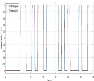
(3) Figure 2: Schematic representation of the prototype hydraulic canal λ = 0.85 .. G(s) =. K 1 + T sλ. e−Ls. (1). 3.2 Characteristics and design of PRBS A Pseudorandom binary signal (PRBS) finds applications over many disciplines for system identification. The frequency spectrum of the PRBS is known as an approximation of the limited bandwidth of the white noise, and then it represents a useful stimulus for frequency response analysis. By definition, the PRBS consists of a random se-. Figure 3: PRBS signal designed according to the system constraints. quence of binary states that usually generated by means of a shift register with feedback paths. The size of the sequence (M) depends on the number of. • The time duration of the PRBS signal can be. bits (N) of the shift register and the positions of the. defined as, the shorter necessary time needed. feedback paths.. by the impulsive response, of such system, to reach and stabilize into the zero value. This. 3.2.1 PRBS generation. theoretical value can be assured according to. The PRBS signal of Figure 3 has been designed ac-. equation :. cording to the following system constraints: D PRBS > 3 T + L. (2). • The frequency of the PRBS signal is fixed to cover the bandwidth of the considered system.. In the case of the hydraulic canal system, we. In the case of our model, the time constant is. are taking into account the time delay of the. T = 1.82s, the bandwidth that covers the sys-. system approximated by L = 4.95 s, the delay. tem frequencies is BW = 5.4H z and then, the. caused by the gate translations each time a. period of the PRBS is T PRBS = 1.2s.. new reference is applied to the system. Also,. 690.

(4) we are considering the sampling time of the system. In order to precisely reproduce the impulsive response of the considered model, the number of samples per period for the PRBS signal has to be enough. Accordingly, an additional time has been added to the periodicity of the PRBS signal and the new time duration of the PRBS signal is now: D = 15s. The number of bits associated with the periodicity of the PRBS signal is concluded from equation (3). 2n−1 = D PRBS , n = 4.90;. (3) Figure 4: PRBS signal affected by the gate model. The number of bits has been concluded then equal to 5, and the length of the PRBS signal corresponding is D = 31s. 3.2.3. Quantization model. • The sampling time of the system is h = 0.13s.. The sensors of the hydraulic canal system charac-. • The amplitude of the PRBS signal equal to. terised by a resolution factor equal to 0.05mm. Accordingly, a quantizer block is used to model this. 1mm.. resolution and the obtained signal will be modified 3.2.2 Gate model. according to the following equation where ys rep-. In order to achieve the time domain identification. resents the output of the system, yq represents the output of the quantization model , r = 0.05 repre-. by using the PRBS signal, the upstream gate dy-. sents the resolution of the sensors, the nearest in-. namics were analyzed, and a new gate model has. teger function is defined such that nint(x) is the. been developed and showed in equation (4), where. integer closest to x .. the aim is to improve the identification performances. In that equation, YG∗ represents the gate. yq = r ∗ nint. reference, YG represents the actual position of the. .. (y ). gate, YG represents the derivative of the gate position, and ν represents the velocity of the gate.  ( ) . ν si gn YG∗ − YG , YG = 0,. if YG∗ ̸= YG if YG∗ = YG. 4. s. r. (5). Simulation results. In this section, simulations results have been ob-. (4). tained using the identification procedure described in this work and the models of the fractional-order. These dynamics could affect the linearity of the. model of the hydraulic canal system, the model of. system, certainly that the period of the PRBS sig-. the upstream gate, and the resolution of the sensor. nal is very small compared to the final time of a. developed on Simulink Matlab.. step signal. The new signal that reaches the model of the hydraulic canal system is detailed in Fig-. First, the PRBS signal already defined in the pre-. ure 4 in red color, the injected PRBS signal repre-. vious part is used as an input signal, the gate. sented in blue color to put the accent into the real. model affect the input according to Figure 4, and. function of the Gate model, how much the refer-. the output signal is quantized with an order corre-. ence signal can be affected by that model and by. sponding to the resolution of the sensor. The im-. the way the improvement of the final model for the. pulsive response of the system has been concluded. considered system.. from the cross-correlation function of the two sig-. 691.

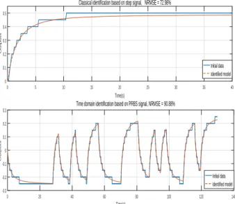
(5) nals (input and output). The obtained fractional-. fractional-order transfer function. The elaborated. order model appears in table 1 in the first posi-. identification procedure was based on time domain. tion and in order judge the precision of the new. data, PRBS signal has been considered according. approximated model, time responses are compared. to the model parameters, the new improvements to. with that corresponding to the reference model in. the system in relation with the real components of. Figure 5. In addition, The performance is deter-. our hydraulic canal, and the sampling time of the. mined with the Normalized Root Mean Square Er-. system. A new model has been developed for the. ror (NRMSE) defined by the equation (6), where yr. upstream gate in order to read precisely the ref-. is the response of the reference model and yap p is. erences data injected to the system, and another. the response of the identified model for the same. modelization has been carried out in accordance to. input.. the sensor’s resolution in order to carefully mea(. NRMSE = 100 1 −. ° ° ° yr − yap p °. sure the output obtained signal.. ). (6). ∥ yr − mean (yr )∥. Using the output signal to an input of form PRBS, the impulsive response of the system is concluded. In the second case, the input is a step signal of an. from the cross-correlation of the two signals, the. amplitude equal to 2 mm and a final time equal to. transfer function is obtained, and the identifica-. 40 s. In both cases, the output signals have been. tion procedure has been discussed in comparison. saved.. with another identification carried out by a step signal. Classical identification based on step signal, NRMSE = 72.98%. 0.5. In order to prove the added value and the benefits. Outputs. 0.4. from using a PRBS input signal on system identifi-. 0.3. cation procedure, a new aleatory signal was used to. 0.2. justify the precision of the obtained model and ac-. Initial data Identified model. 0.1. cordingly, the normalized root mean square error. 0 0. 5. 10. 15. 20. 25. 30. 35. 40. Time(s). Time domain identification based on PRBS signal, NRMSE = 90.88%. confirm in percent how much improve this technic the model of the hydraulic canal.. 0.3 0.2. Outputs. 0.1. Acknowledgement. 0 -0.1. Initial data Identified model. -0.2. NO acknowledgements.. -0.3 0. 20. 40. 60. 80. 100. 120. 140. Time(s). References. Figure 5: Fractional-order Identification based on PRBS and step signals for the new system model. [1] B. T. Krishna and K. V. V. S. Reddy, (2008) Active and passive realization of fractance de-. Table 1: Model parameters obtained by time domain. vice of order, Active and Passive Electronic. identification in comparison with the classic identification based on step signal Input signal PRBS Step. Kf 0.26 0.246. Lf 4.95 4.95. Tf 1.72 1.73. λ. 0.76 0.84. Components, Article ID 369421, 5 pages.. NRMSE 90.88% 72.98%. [2] G. W. Bohannan,(2008) Analog fractional order controller in temperature and motor control applications, Journal of Vibration and Control, vol. 14, pp 1487-1498.. 5 Conclusions [3] H. H. Sun, B. Onaral, Y. Tsao,(1984) ApplicaThis article has addressed the identification of. tion of positive reality principle to metal elec-. the laboratory hydraulic canal model by a delayed. trode linear polarization phenomena, IEEE. 692.

(6) Trans. Biomed. Engrg. BME-31 (10) pp 664-. model of an irrigation main canal pool, Span-. 674.. ish Journal of Agricultural Research, Volume 13, Issue 3, e0212.. [4] J. Cervera and A. BaËœnos,(2008) Automatic loop shaping in QFT using CRONE struc-. [14] T.. T.. Hartleya,. C.. F.. Lorenzob,(2003). tures, Journal of Vibration and Control, vol.. Fractional-order system identification based. 14, pp 1513-1529.. on continuous order-distributions,. Signal. Processing, pp 2287-2300.. [5] J. De Espindola, C. Bavastri, and E. De Oliveira Lopes, (2008) Design of optimum sys-. [15] V. F. Batlle, A. S. Millan and R. R. Perez,. tems of viscoelastic vibration absorbers for a. (2017) Multivariable Fractional-order Model. given material based on the fractional calcu-. of a Laboratory Hydraulic Canal with two. lus model, Journal of Vibration and Control,. Pools, Proceedings of 4th International Con-. vol. 14, pp 1607-1630.. ference on Control, Decision and Information Technologies (CoDIT’17) / April 5-7, 2017,. [6] J. Rosario, D. Dumur, and J. T. Machado,. Barcelona, Spain.. (2006) Analysis of fractional-order robot axis dynamics, in Proceedings of the 2nd IFAC. [16] V. Feliu, S. Feliu, (1997) A method of obtain-. Workshop on Fractional Differentiation and. ing the time domain response of an equiva-. Its Applications, vol. 2.. lent circuit model, Journal of Electroanalydcal Chemistry, 435, pp 1-10.. [7] M. F. M. Lima, J. A. T. Machado, and M. Crisostomo, (2007) Experimental signal anal-. [17] V. Feliu, J. A. Gonzalez, S. Feliu, (2004) Al-. ysis of robot impacts in a fractional calculus. gorithm for extracting corrosion parameters. perspective, Journal of Advanced Computa-. from the response of the steel-concrete sys-. tional Intelligence and Intelligent Informat-. tem to a current pulse, Journal of The Elec-. ics, vol. 11, pp. 1079-1085.. trochemical Society, 151 pp 134-140.. [8] M. H. Chaudhry, (2008) Open-channel flow,. [18] Y. Y. Tsao, B. Onaral, H. H. Sun,(1989) An. 2nd ed. New York: Springer.. algorithm for determining global parameters. [9] N. M. M. Maia, J. M. M. Silva, A. M. R.. of minimum-phase systems with fractional. Ribeiro, (1998) On a general model for damp-. power spectra, IEEE Trans. Instrum. Meas,. ing, J. Sound Vib. 218 (5), pp. 749-767.. pp 723-729.. [10] R. E. Gutierrez, J. M. Rosario, and J. T.. [19] Z. Z. Yang and J. L. Zhou,(2008) An improved. Machado,(2010) Fractional Order Calculus:. design for the IIR-type digital fractional or-. Basic Concepts and Engineering Applica-. der differential filter, in Proceedings of the. tions, Mathematical Problems in Engineer-. International Seminar on Future Bio-Medical. ing, Article ID 375858, 19 pages.. Information Engineering (FBIE 08), pp 473476.. [11] R. L. Magin and M. Ovadia, (2008) Modeling the cardiac tissue electrode interface using fractional calculus, Journal of Vibration and Control, pp 1431-1442.. © 2018 by the authors. Submitted for possible open access pub-. [12] R. Panda and M. Dash,(2006) Fractional gen-. lication under the terms and. eralized splines and signal processing, Signal. conditions of the Creative Commons Attribution CC-BY-. Processing, vol. 86, pp 2340-2350.. NC 3.0 license (http://creativecommons.org/licenses/bync/3.0/).. [13] S. N. Calderon-Valdez, V. F. Batlle and R. R. Perez, (2015)Fractional-order mathematical. 693.

(7)