Learning Curve in Make To Order and Make To Stock Logistics Management Approaches

Texto completo

(1)LEARNING CURVE IN MAKE-TO-ORDER AND MAKE-TO-STOCK LOGISTICS MANAGEMENT APPROACHES Dipl.-Ing. Yalili Rodríguez Romero Industrial Engineering Department, Central University from Las Villas, Cuba Dr. Roberto Cespón Castro Industrial Engineering Department, Central University from Las Villas, Cuba Prof. Dr.-Ing. Dr. h.c. Norge Isaias Coello Machado Mechanical Engineering Department, Central University from Las Villas, Cuba Dr.-Ing. Elke Glistau Institute of Logistics and Material Handling Systems, Otto von Guericke University, Germany Abstract Knowledge is a strategically valuable resource in business management. Activity repetition is known to help learning and improve the ability to do certain job with better quality, lower time consumption and consequently, at lower production cost. This learning ability allowed the development of a prediction technique known as the "learning curve". This technique has been applied in different production processes for planning and to consider the impact on productivity, quality of work. This research is based on the possibility to extrapolate the concept of the learning curve to the supply chain and more specifically to its lead-time. Leadtime is understood as the period of time between the request of an order by the customer and the time when it is satisfied. Therefore, this paper describes a methodology to extrapolate the concept of the learning curve to the supply chain. Firstly, the logistics network is described. Then a pilot sample of orders is determined, for which the lead-time is estimated according to the logistic management approaches (make to order and make to stock) in two Cuban companies. Subsequently, the sample size is verified by statistical regression. Conversion factors for the "learning curve" are determined, and the expected lead-time is adjusted in future orders. Consequently, the essential objective of this paper is to realize the learning curve to measure the leadtime of the orders, for the MTO and MTS logistics management approaches. Keywords: Supply chain; Lead-time; Learning curves. 1 Introduction The current scenario presupposes the adoption of new strategies of competitiveness on the part of the businessmen oriented to fulfill the expectations of the customer to offer them better products and services, decreasing the lead time. This requires shorter and less expensive lean-time, where the. consideration of learning and its determination offer very promising expectations. It is known that by repeating an activity, you learn and the subject has the ability to do your job faster with better quality and lower cost of the product. This learning ability allowed the development of a prediction technique known as the "learning curve", first observed in [1] Since then, this technique has been applied in different production processes to consider the impact on productivity and quality of work and its incorporation in production planning. In [2], a knowledge creation framework is proposed, in which internal and external learning is directly related throughout the supply chain. It states that manufacturers would do well to allocate their resources to support and implement learning routines and strive to become a learning organization. This research is based on the fact that it is possible to extrapolate the concept of learning curves to the supply chain and more specifically to its lead-time. In this way, the supply chain involves not only production processes, but also storage and transport; for this reason, the problem to solve in the present investigation is the elaboration of a learning curve. Objective is to realize the learning curve to measure the lead-time of the orders. Two companies are taken as objects of study, one belonging to the construction industry: (A) and the other one, to the chemical industry: (B). This document is structured in five sections. In the next section, research background shows the literature analysis. First, the supply chain using management approaches and what the learning curve is. Section three proposes a methodology for the calculation of the learning curve in the selected study cases. Results and conclusions are shown in sections four and five, respectively. 2 Research background.

(2) 2.1 Supply chain This investigation starts from supposing a relationship between the supply chain and more specifically the duration of the lead-time with the generation of knowledge and learning measured through the learning curves. For this it is important to emphasize that the focus of the management of processes and operations, is based on maximizing profit, reducing costs through the automation of processes and the production of large volumes of manufacturing [3]. In [4] it is considered that developed a classification to characterize the different structures of supply chains and following this classification, in [5] it is proposed a framework based on the structures of the supply chain and two main contextual factors. At the same time, four logistic management approaches are recognized: make to stock (MTS), make to order (MTO), and engineering to order and assemble to order. For the purposes of the presented work, the MTO and MTS are of interest. Each one of them presents distinctive characteristics according to the dynamics of the production and the challenges for its management. MTS is based on demand forecasts and is generally used to produce generic and high turnover products [6]. On the other hand, MTO responds exclusively to signed orders and allows greater product flexibility, although with a longer response time [7]. The SCOR model developed by the Supply-Chain Council (SCC) in 1996 visualizes the supply chain of an organization from the supplier of suppliers to the customer of customer, including the relationships between internal customer [8], [9], [10], [11]. The SCOR model at its three levels, provides key performance indicators, systematically divided into five attributes: reliability or reliability in compliance, agility or flexibility, responsiveness, cost and asset management [10], [11]. The strategic metric to evaluate responsiveness is the order fulfillment lead-time. This model also recognizes the MTS, MTO, and the engineering to order (ETO) as main work environments. In [12] it is argue an important issue that is not abundant in the literature of the supply chain is related to the influence of the human factor and its knowledge. In [13] is suggested that with the fourth industrial revolution, the separation between materials and information will disappear, because information will be an intrinsic part of the products. 2.2 Learning curves Effects of learning have been investigated frequently in recent years. Wright in 1936 showed. that the average unit production costs in aircraft assembly are reduced depending on the number of aircraft produced. This phenomenon is caused by an increase in the skill levels of the worker and a decreasing number of errors [14]. Doing an activity after the first time involves learning, product of experience. The learning curve is a characteristic inherent in all organized activity [15]. Learning curve can be studied through two perspectives, which have as a reference are costs [16]. First, costs are reduced as the volume of production increases and second, total costs decline in a production line as the volume of production increases. Learning curve is no more than a line that shows the relationship between the time (or cost) of production per unit and the number of consecutive production units [17]. In [18], it is made a historical review of the learning curves and explains that the literature on the subject focuses on military issues in the period from 1935 to 1969 and only after 1970 are studies focused on the strategic direction in the industry, product of its application by Boston Consulting Group (BCG) and Conley. Since 2000, learning curves in organizations have been used as a forecasting tool and a calculation of the costs generated by different treatments can be done, which shows that there are different models to explain learning in companies [19]. In 2002-2003, learning curves are used and control limits are generated for defective products, through a treatment in the learning period of a manufacturing company [20], [21]. The effects of the learning process in an industrial context have been verified in a series of studies; however, the focus was on the production process in most cases, and not on logistics processes. In [22] it is proposed to link the effects of learning with activities that include ordering forms in a warehouse. This is confirmed in [23] the review of the literature where he states that of the 457 articles consulted only thirteen are supply chain and one is dedicated to logistics. Therefore, learning curve has little studies on processes of the supply chain and specifically in the lead-time. In [24] is suggested the realization of different models of learning curve in the light of new technologies and emerging industries, giving the example in the fourth industrial revolution. Considering that lead-time is an activity that includes provisioning, production and commercialization as a result of repetitive investigations, it can be assumed that lead time reduces with learning over time..

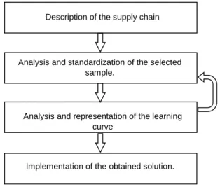
(3) 3. Methodology for learning curves. the. determination. of. In this section, we propose a methodology to determine the learning curve in lead-time. To achieve this goal we follow the procedure shown in figure 1.. Afterward, it is accumulate the quantities of products and the duration of the cycle to avoid that the difference in the quantities affects the result. Finally, the cumulative duration is multiplied by eight working hours, and divided; by the accumulated quantity of products. 3.3 Analysis and representation of the learning curve. Description of the supply chain. In the analysis of the sample, it is taken into account if the selected size is feasible, an analysis of the different regression equations is made. Maximum permissible errors are established through the confidence intervals of the established parameter. Then determine the learning curve and the learning ratio using the logarithmic method (equation 2 and 3) taking into account the analogies of table 1. The logarithmic method is the most used according to the study [23].. Analysis and standardization of the selected sample.. Analysis and representation of the learning curve. Implementation of the obtained solution.. Figure 1: Methodology for the determination of learning curves. 3.1 Description of the supply chain First, supply chain is described and represented. Then the production approach is determined with it is considered by the SCOR model (MTO and MTS). 3.2. Analysis and standardization selected sample. of. the. For the selection and standardization of the sample, the different production approaches are taken into account. In the MTO system, a typical representative is chosen one according to the quantity of products and their complexity. From this, the reduction coefficient (equation 1) is calculated to know the percentage of time that each article represents with respect to the representative type (Nt type). Where ki is the coefficient of product reduction and Nt is total time rule for the product i. Product representative type is the window. Then orders are homogenized by multiplying each coefficient by the number of items of each type requested in the orders. Contracts are analyzed with their start dates and receipt of invoices, as well as the required demand. In the MTS system, the lead-time is divided into two parts. First, the duration of the part corresponding to the production-commercialization cycle is determined and the supply time is estimated by statistical simulation.. 𝐍𝐭 𝐍𝐭 𝐭𝐲𝐩𝐞 𝒀𝒏 = 𝒌 ∗ 𝒙𝒃 𝐥𝐨𝐠(𝒓) 𝒃= 𝒍𝒐𝒈𝟐 𝐤𝐢 =. (1) (2) (3). 3.4 Implementation of the obtained solution When the learning curve is obtained, a small economic analysis is made. By change the reason for learning, sensitivity is evaluated and its impact on lead time. Then, conversion factors are tabulated as a decision support tool for managers. 4 Results Company "A" has three main suppliers, five customer and 111 workers. The analyzed products are pre-construction. Window is the typical representative of his production. "B" has ten main suppliers, six customer and 258 workers. In the investigation of analyze three types of detergent that are elaborated here. Table 2 shows the behavior of the coefficient of determination of all the regression equations. The best equation is power because it has the highest coefficient of determination. The slope hypothesis test is performed to determine the quality of the adjustment to the regression. The p-value is lower than the level of significance of 0.05 set in the study. Regression is significant. Confidence intervals are calculated in MTO is [8.09; 9.22] with a maximum permissible error of 0.56 days / unit. In MTS the interval is [84.0; 89.8] with an error of 2.77 hours / 1000-units..

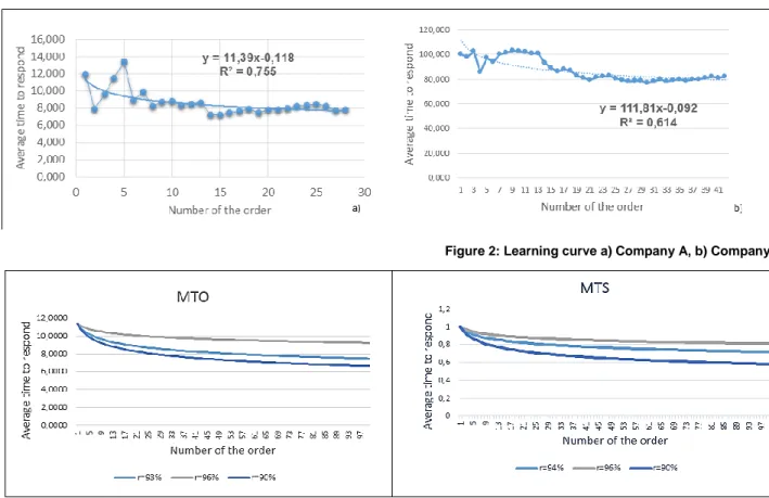
(4) Variable X Yn. Production Consecutive number of the product Average time (in hours) for the production of product X. k. Working time for finishing the production of the first product. Criterion established when the number of orders is doubled, to establish the learning rate Equation coefficient Learning curve rate. log 2 b r. Lead-time Consecutive order number Average time (in hours) for the duration of the lead-time of the order X Average time of the lead-time to finish the first order.. Table 1: Modifications made to the logarithmic method for the determination of learning in the lead-time. Models Power Cubic Quadratic Logarithmic Compound Growth Exponential Logistics Linear S Inverse. R 0.86 0,70 0,70 0,66 0,60 0,60 0,60 0,60 0,59 0,57 0,56. MTO R2 0.75 0,49 0,49 0,43 0,36 0,36 0,36 0,36 0,35 0,32 0,29. R 0,78 0,76 0,76 0,68 0,74 0,74 0,74 0,74 0,70 0,42 0,42. MTS R2 0,61 0.57 0.57 0,46 0.54 0.54 0.54 0.54 0.49 0,18 0,17. Table 2: Coefficients of the regression equations. Learning curve for the lead-time in companies "A" and "B" is shown in figure 2. Coefficients of determination are 0.755 and 0.614, values that represent a good adjustment. Reason for learning is 93% and 94% respectively. Average of errors is 0.019 and 0.053 respectively when analyzing the errors of the equation. Errors what are considered valid and brought about mainly by the differences in the characteristics of the supply, the condition of the market and the great fluctuation of the labor force present in "A" and "B". Finally, figure 2 depicts that there is a decreasing trend in the curve as the number of orders increases, which indicates that learning is present.. Figure 2: Learning curve a) Company A, b) Company B. Figure 3: Duration of the lead-time with different learning rates. Once the curve is obtained, it is possible to readjust the lead-time, starting from the fact that as more homogenized orders are made and learning is considered, the time must be reduced. In fact, if you want to know the expected duration of a future order 29 in "A" the value of K is replaced in equation 2, you get 7,83 days / unit. This value means that the order 29 of a homogenized unit will be delayed under the learning effect 8 days.. To know the total duration of the real lead-time, it would be sufficient to multiply the value obtained by the quantity of homogenized units of the order. Final value obtained would be the lead-time to be promised to the customer. Similarly, in "B" if you analyze order 23 that took 24 days, for 2000 units and report an income of $ 10013.60. If the learning is considered using the conversion factor of 0.8176; then, conversion.

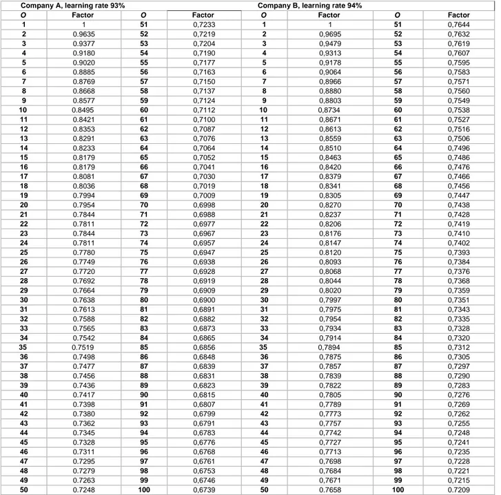
(5) factor is multiplied by 111.78 which is the average duration of the first order and 91.39 hours per 1000 units that will be obtained 182.78 hours to use for the entire order, 9.22 hours less than those actually used. This generates an increase of $ 480.86. If this time is used to comply with other orders, a difference between the companies in the sector is established. Company A, learning rate 93% Factor O 1 1 2 0.9635 3 0.9377 4 0.9180 5 0.9020 6 0.8885 7 0.8769 8 0.8668 9 0.8577 10 0.8495 11 0.8421 12 0.8353 13 0.8291 14 0.8233 15 0.8179 16 0.8179 17 0.8081 18 0.8036 19 0.7994 20 0.7954 21 0.7844 22 0.7811 23 0.7844 24 0.7811 25 0.7780 26 0.7749 27 0.7720 28 0.7692 29 0.7664 30 0.7638 31 0.7613 32 0.7588 33 0.7565 34 0.7542 35 0.7519 36 0.7498 37 0.7477 38 0.7456 39 0.7436 40 0.7417 41 0.7398 42 0.7380 43 0.7362 44 0.7345 45 0.7328 46 0.7311 47 0.7295 48 0.7279 49 0.7263 50 0.7248. O 51 52 53 54 55 56 57 58 59 60 61 62 63 64 65 66 67 68 69 70 71 72 73 74 75 76 77 78 79 80 81 82 83 84 85 86 87 88 89 90 91 92 93 94 95 96 97 98 99 100. Factor 0,7233 0,7219 0,7204 0,7190 0,7177 0,7163 0,7150 0,7137 0,7124 0,7112 0,7100 0,7087 0,7076 0,7064 0,7052 0,7041 0,7030 0,7019 0,7009 0,6998 0,6988 0,6977 0,6967 0,6957 0,6947 0,6938 0,6928 0,6919 0,6909 0,6900 0,6891 0,6882 0,6873 0,6865 0,6856 0,6848 0,6839 0,6831 0,6823 0,6815 0,6807 0,6799 0,6791 0,6783 0,6776 0,6768 0,6761 0,6753 0,6746 0,6739. By performing a sensitivity analysis (figure 3) of the order cycle time and varying, the level of learning we can observe the decrease or increase of the lead-time. In this paper, managers are offered a tool for practical solution to calculate the duration of the lead-time taking into account the learning. Table 3 shows the tabulated conversion factors. Company B, learning rate 94% Factor O 1 1 2 0,9695 3 0,9479 4 0,9313 5 0,9178 6 0,9064 7 0,8966 8 0,8880 9 0,8803 10 0,8734 11 0,8671 12 0,8613 13 0,8559 14 0,8510 15 0,8463 16 0,8420 17 0,8379 18 0,8341 19 0,8305 20 0,8270 21 0,8237 22 0,8206 23 0,8176 24 0,8147 25 0.8120 26 0,8093 27 0,8068 28 0,8044 29 0,8020 30 0,7997 31 0,7975 32 0,7954 33 0,7934 34 0,7914 35 0,7894 36 0,7875 37 0,7857 38 0,7839 39 0,7822 40 0,7805 41 0,7789 42 0,7773 43 0,7757 44 0,7742 45 0,7727 46 0,7713 47 0,7698 48 0,7684 49 0,7671 50 0.7658. O 51 52 53 54 55 56 57 58 59 60 61 62 63 64 65 66 67 68 69 70 71 72 73 74 75 76 77 78 79 80 81 82 83 84 85 86 87 88 89 90 91 92 93 94 95 96 97 98 99 100. Factor 0,7644 0,7632 0,7619 0,7607 0,7595 0,7583 0,7571 0,7560 0,7549 0,7538 0,7527 0,7516 0,7506 0,7496 0,7486 0,7476 0,7466 0,7456 0,7447 0,7438 0,7428 0,7419 0,7410 0,7402 0,7393 0,7384 0,7376 0,7368 0,7359 0,7351 0,7343 0,7335 0,7328 0,7320 0,7312 0,7305 0,7297 0,7290 0,7283 0,7276 0,7269 0,7262 0,7255 0,7248 0,7241 0,7235 0,7228 0,7221 0,7215 0.7209. Table 3: Conversion factors. 5 Conclusions Considerations and results obtained allow determining the duration of the lead-time and the realization of the learning curves. Learning process is used as a forecasting method to determine lead times should be a commitment to customers by reducing the logistics costs of the supply chain. Sensitivity analysis demonstrates the variation between the different levels of learning and the. duration of the final lead-time. In this research, tabulated conversion factors are also offered to facilitate the work of specialists. Results of this study have limitations (see also [25]), because the attributes of the learning curve depend on a variety of factors, such as in the selected process, the characteristics of the individuals and the work environment. However, it was shown that while the number of orders.

(6) increases, learning begins to show in the lead-time analyzed. In future paper would be interesting to carry out similar studies in the engineering to order and assemble to order; approaches not addressed in the case studies.. [12]. [13]. 6 Reference [1]. [2]. [3]. [4]. [5]. [6]. [7]. [8]. [9]. [10]. [11]. T. P. Wright, "Factors affecting the cost of airplanes," Journal of aeronautical sciences, vol. 3, pp. 122-128, 1936. X. Huang, M. M. Kristal, and R. G. Schroeder, "Linking learning and effective process implementation to mass customization capability," Journal of Operations Management, vol. 26, pp. 714-729, 2008. R. Sanchis and R. Poler, "Estrategias de Gestión de los Procesos y Operaciones en Escenarios de Personalización en Masa," in 4th International Conference On Industrial Engineering and Industrial Management, 2011, pp. 1248-1257. R. Ernst and B. Kamrad, "Evaluation of supply chain structures through modularization and postponement," European journal of operational research, vol. 124, pp. 495-510, 2000. A. Brun and M. Zorzini, "Evaluation of product customization strategies through modularization and postponement," International Journal of Production Economics, vol. 120, pp. 205-220, 2009. H. Rafiei and M. Rabbani, "Order partitioning in hybrid MTS/MTO contexts using fuzzy ANP," Engineering and Technology, vol. 4563, pp. 467-472, 2009. C.-S. Chen, S. Mestry, P. Damodaran, and C. Wang, "The capacity planning problem in make-to-order enterprises," Mathematical and computer modelling, vol. 50, pp. 1461-1473, 2009. E. Arenas, "Análisis de la cadena de suministro por medio del modelo SCOR," Contacto Industrial, pp. 3-8, 2007. B. Hitpass, BPM: Business Process Management: Fundamentos y Conceptos de Implementación 4a Edición actualizada y ampliada: Dr. Bernhard Hitpass, 2017. S. A. Rozo Zamora, "Propuesta de implementación del modelo Scor en la empresa Sotracarga Ltda," 2015. F. Salazar, J. Cavazos, and J. L. Martínez, "Metodología basada en el Modelo de Referencia para Cadenas de Suministro para Analizar el Proceso de producción de Biodiesel a partir de Higuerilla," Información tecnológica, vol. 23, pp. 47-56, 2012.. [14]. [15]. [16]. [17]. [18]. [19]. [20]. [21]. [22]. [23]. [24]. [25]. M. Khan, M. Y. Jaber, and A.-R. Ahmad, "An integrated supply chain model with errors in quality inspection and learning in production," Omega, vol. 42, pp. 16-24, 2014. E. Glistau and N. I. Coello Machado, "Industry 4.0, logistics 4.0 and materialsChances and solutions," in Materials Science Forum, 2018, pp. 307-314. E. H. Grosse, C. H. Glock, and S. Müller, "Production economics and the learning curve: A meta-analysis," International Journal of Production Economics, vol. 170, pp. 401-412, 2015. W. B. Hirschmann, "Profit from the learning-curve," Harvard Business Review, vol. 42, pp. 125-139, 1964. W. J. Abernathy, "Limits of the learning curve," Harvard Business Review, vol. 52, pp. 109-119, 1974. A. C. Hax and N. S. Majluf, "Competitive cost dynamics: the experience curve," Interfaces, vol. 12, pp. 50-61, 1982. L. E. Yelle, "The learning curve: Historical review and comprehensive survey," Decision sciences, vol. 10, pp. 302-328, 1979. M. Texis Flores, A. Mungaray Lagarda, M. Ramírez Urquidy, and N. Ramírez Angulo, "Aprendizaje en microempresas de Baja California," Estudios fronterizos, vol. 12, pp. 95-116, 2011. V. Kumpikaite, "Human resource development in learning organization," Journal of business economics and management, vol. 9, pp. 25-31, 2008. S. C. Council, "Supply chain operations reference model," Overview of SCOR version, vol. 5, 2008. E. H. Grosse and C. H. Glock, "An experimental investigation of learning effects in order picking systems," Journal of Manufacturing Technology Management, vol. 24, pp. 850-872, 2013. C. H. Glock, E. H. Grosse, M. Y. Jaber, and T. L. Smunt, "Applications of learning curves in production and operations management: A systematic literature review," Computers & Industrial Engineering, 2018. C. H. Glock, E. H. Grosse, M. Y. Jaber, and T. L. Smunt, "Novel applications of learning curves in production planning and logistics," Darmstadt Technical University, Department of Business Administration …2019. B. Hitchings and D. Towill, "An error analysis of the time constant learning curve model," THE INTERNATIONAL JOURNAL OF PRODUCTION RESEARCH, vol. 13, pp. 105-135, 1975..

(7)