New Estimation Techniques in Commodity Derivative Models under the Risk neutral Measure

Texto completo

(1)PROGRAMA DE DOCTORADO EN ECONOMíA. TESIS DOCTORAL: New Estimation Techniques in Commodity Derivative Models under the Risk-neutral Measure Nuevas Técnicas de Estimación en Modelos de Derivados de Materias Primas bajo la Medida Neutral al Riesgo. Presentada por Ziba Habibi Lashkari para optar al grado de Doctora por la Universidad de Valladolid. Dirigida por: Lourdes Gómez del Valle Julia Martínez Rodríguez.

(2)

(3) Supervisors: Lourdes Gómez del Valle Julia Martı́nez Rodrı́guez. Examination board:. Dean of the Factulty of Economics and Business:. Rector of the University of Valladolid:.

(4)

(5) Acknowledgements First and foremost, I want to thank my advisors, Dr. Lourdes Gómez del Valle and Dr. Julia Martı́nez Rodrı́guez. It has been an honor to be their Ph.D. student. Their guidance helped me in all the time of research and writing of this thesis. I could not have imagined having better advisors and mentors for my Ph.D. study. I would like to express my special appreciation and thanks to Dr. José Luis Garcı́a Lapresta, you have been a tremendous mentor for me. I would like to thank you for encouraging my research and for allowing me to grow as a research scientist. Your advice on my career has been priceless. I would especially like to thank Dr. Pierre Six at Neoma Business School, Rouen, France who provided me an opportunity to join his team as a researcher, and who gave me access to the research facilities. Without his precious support, it would not be possible to conduct this research. I met amazing people in Rouen. Thanks to everyone, especially Jungsun Cho, Peiran Guo, and Lei Yin at the Neoma Business School who supported me through good and bad times. Thanks to professors from Neoma and their organization who worked with me over those three months. I appreciate all their contributions of time and ideas to make my Ph.D. experience productive and stimulating. The joy and enthusiasm they have for their research was contagious and motivational for me, even during tough times in the Ph.D. pursuit. Special thanks to all professors in the Faculty of Economics and Business at UVa have contributed immensely to my personal and professional time. This group has been a source of friendships as well as good advice and collaboration. Nobody has been more important to me in the pursuit of this project than the members of my family. I would like to thank them for all their love and encouragement. For my parents who raised me with a love of science and supported me in all my pursuits. Words cannot express how grateful I am to my mother, father and my brother for all of the sacrifices that they have made on my behalf. This work would not have been possible without the financial support of my parents. A special acknowledgment goes to my office mate of many years: Veronica Arredondo. She was a real friend ever since we began to share an office in 2015. Veronica is an amazing person in too many ways. I also thank Raquel González, my other great office mate who has been supportive in every way. I would like to express my very great appreciation to my friends. Their unconditional support has been essential all these years. I am not sure I would continue at UVa without their encour-.

(6) agement. I must express my very profound gratitude to my Spanish friends and families which our friendship began in Valladolid and became ripe throughout my years at UVa. Thank you for providing me with unfailing support and constructive recommendation throughout my years of study. This accomplishment would not have been possible without you. Ziba Habibi Lashkari University of Valladolid April 2018.

(7) Contents Acknowledgements. iii. 1 Introduction. 1. 1.1. Commodity markets . . . . . . . . . . . . . . . . . . . . . . . . . . . . . . . . . . .. 2. 1.2. Spot and futures prices . . . . . . . . . . . . . . . . . . . . . . . . . . . . . . . . . .. 3. 1.3. Valuation models . . . . . . . . . . . . . . . . . . . . . . . . . . . . . . . . . . . . .. 4. 1.4. Methodology . . . . . . . . . . . . . . . . . . . . . . . . . . . . . . . . . . . . . . .. 6. 1.5. Contributions . . . . . . . . . . . . . . . . . . . . . . . . . . . . . . . . . . . . . . .. 7. 2 Introducción. 9. 2.1. Los mercados de materias primas . . . . . . . . . . . . . . . . . . . . . . . . . . . .. 10. 2.2. Los precios al contado y los futuros . . . . . . . . . . . . . . . . . . . . . . . . . . .. 11. 2.3. Modelos de valoración . . . . . . . . . . . . . . . . . . . . . . . . . . . . . . . . . .. 13. 2.4. Metodologı́a . . . . . . . . . . . . . . . . . . . . . . . . . . . . . . . . . . . . . . . .. 15. 2.5. Contribuciones . . . . . . . . . . . . . . . . . . . . . . . . . . . . . . . . . . . . . .. 16. 3 A new technique to estimate the risk-neutral processes in jump-diffusion commodity futures models. 19. 4 The jump size distribution of the commodity spot price and its effect on futures and option prices. 29. 5 A multiplicative seasonal component in commodity derivative pricing. 41. Conclusions. 57. Conclusiones. 61. Bibliography. 65. v.

(8)

(9) Chapter 1. Introduction Commodity markets are very important for different industries. On the one hand, they are fundamental to production companies which look for hedging unwanted commodity exposure. On the other hand, they are very interesting for investors who use commodities as investments, Back and Prokopczuk [4]. Moreover, the importance of commodity markets has increased considerably since the start of this century. As a result, they are of great interest for researchers. Recent developments in commodity prices have been atypical in many ways. From the mid2000s a rising trend of commodity prices was observed in the markets. In fact, the boom between 2002 and mid-2008 was the most important one in several decades, both in magnitude and duration. After the beginning of the current global crisis, the prices started to decline and this fact affected a large number of commodities. However, on the whole, since 2009, and especially since the summer of 2010, global commodity prices started to increase again. During this period of time, commodity prices also had a high volatility. These developments also coincide with important changes in commodity market basics. For example, changes in fundamental supply and demand relationships, especially in emerging economies which are experiencing a fast growth. In addition, the aim to reduce the use of fossil fuels in energy consumption, the debate about global climate change and its link with agricultural production has had an important impact on recent commodity price evolution. However, these factors are not enough to explain the behaviour of commodity prices. In fact, the greater presence of financial investors in these markets looking to diversify their portfolios beyond traditional securities, is an additional factor. This phenomenon is called financialization of commodity markets and its importance has increased considerably since 2004, as can be perceived by the rising volume of financial investments in commodity derivative markets. This situation is important because the activity of these financial participants can move commodity prices away from the levels fixed by supply and demand relationships. Financial investors make trading decisions based on factors not totally related to the corresponding commodity, such as portfolio considerations or following the market trend. Moreover, this fact can have negative effects on both the consumers and producers 1.

(10) 2. Chapter 1: Introduction. of commodities.. 1.1 Commodity markets Trading in commodity spot markets is quite limited because most market participants look for a financial exposure to the movements of the underlying commodity price instead of the underlying commodity itself. Therefore, as Back and Prokopczuk [4] state: “trading and price discovery take place in the futures markets”. Commodity derivatives are traded on organized exchanges as well as on over the counter (OTC), usually with a financial institution. Futures exchanges where trade standardized clearly defined products, offer higher liquidity, price transparency, and reduce default risk. However, the variety of these exchange-traded standardized contracts is quite limited and they do not always provide a perfect hedge. In the OTC markets, traders can go beyond standardized futures products and customize them in terms of the contracts they trade. Although they offer great freedom and potentially lower trading costs, these markets may leave both parties at risk, if they are not using the services of a clearing house. In fact, currently, OTC markets are still rather opaque in all parts of the world. In the US, the most popular exchanges are those run by the CME Group, which originated after the Chicago Mercantile Exchange (CME) and Chicago Board of Trade (CBT) merged in 2006. The New York Mercantile Exchange (NYMEX) is among its operations. Nowadays, tradable commodities are divided into four categories: • Metals. They are probably the most traded commodities. They can also be divided into various categories, for instance, precious metals (gold, silver, etc.), base metals (copper, aluminum, etc.), carbon, steel and so on. • Energy. It is one of the most influential commodities. It includes crude oil, natural gas, coal and so on. • Agricultural. These are goods such as cotton, cocoa, sugar, orange juice, etc. • Livestock and meat. These commodities include live cattle, feeder cattle and lean hogs and they are more volatile than other traded commodities. A well-known way to invest in commodities is through a futures contract, which is an agreement between two parties to buy (or sell) a specific quantity of a commodity at a fixed specific price and at a predetermined future date on an organized exchange. Another way is through option contracts. Options provide greater flexibility to market participants because they are designed to offer the right (not the obligation) to buy (or sell) a specific commodity or contract at a predetermined specific price and at a given date in the future, see Cummins and Murphy [26]. In financial commodity markets, there are mainly two types of investors:.

(11) 1.2 Spot and futures prices. 3. • Hedgers buy and sell contracts to protect themselves from possible commodity price movements. They try to avoid risks. • Speculators try to make some profit analyzing the commodity markets, forecasting derivative price movements and trading.. 1.2 Spot and futures prices In commodity markets, it is interesting to know the term structure of commodity futures prices, which is the relationship between the futures prices and the maturity for any delivery rate Lautier [54]. In fact, changes in the slope of the commodity futures curves have very important consequences for investment decisions and risk management and have been the focus of numerous studies, see Acharya et al. [1], Bessembinder and Lemmon [13], and Geman and Ohana [35]. A futures curve is upward sloping when futures prices are higher than the spot price and this situation is called contango. On the contrary, when futures prices are below the current spot price the futures curve is downward sloping and this situation is called backwardation. The futures curve can also show a humped shape. Moreover, the shape of the term structure of futures prices changes over time, see for example Hambur and Stenner [42]. The shape of the term structure of the commodity futures curve has been traditionally explained by two broad strands: the theory of storage, which started with Brennan [16], and Kaldor [50] among others, and the hedging pressure literature, which was pioneered by Hicks [45], and Keynes [51]. The theory of storage focuses on the overall benefits of holding the physical commodity and some aspects related to inventories. Owning a commodity provides some benefits, but also some costs. In consequence, the (net) convenience yield is defined as the difference between the gross convenience yield and the costs of holding the physical commodity, such as storage, transportation and so on. According to this theory, there is a relation between the spot and futures prices. If the benefits of holding the commodity (convenience yield) are higher than the financial costs (interest rates), the futures curve is in backwardation. However, if the interest rate is higher than the convenience yield, the futures curve is in contango, see Back and Prokopczuk [4] for more detail. Moreover, holding the physical commodity allows producers to fulfill unexpected changes in demand, avoid temporary shortages of supply and the insurance of the production process, see Kwok [52]. Then, following supply and demand arguments, there is a negative relationship between inventory levels and price, see Back and Prokopczuk [4]. That is, if inventory levels are high, the futures curve is in contango and if inventory levels are low the futures curve is in backwardation. In contrast, the hedging pressure literature focuses on the risk premium. This strand considers that the futures price is the sum of the expected future spot price and risk premium. The theory of normal backwardation proposed by Keynes [51] is based on the general assumption that commodity producers usually want to enter into a short position, because they wish to guarantee a certain.

(12) 4. Chapter 1: Introduction. price level for the delivery. This contract provides a form of insurance against any decline in the spot price to the producers. Thereby, producers are willing to pay a risk premium in order to hedge their exposure. Commodity consumers may also want to protect themselves against increases in the spot price. Then, they will enter into a long position in the futures contract. If the hedging activity of producers of a particular commodity is greater than that of consumers, the futures price will be lower than the expected future spot price and the futures price will be a downward biased estimator of future spot prices, see Back and Prokopczuk [4]. Moreover, this fact will induce speculators to balance the market taking the opposite long position. However, this assumption of hedgers usually being on average in a net short position is not always true. If the hedging activity of consumers is greater than that of producers, there will be an excess of commercial market participants looking to enter a long position, and then, the future price will be above the expected future spot price. In this case, speculators should be compensated for taking a short position in the commodity. Therefore, the futures price may carry either a positive or a negative risk premium depending on the net position of hedgers for each commodity at each moment, see Cootner [25], and Hambur and Stenner [42]. In this sense, Hambur and Stenner [42] define the risk premium as the return that speculators expect to obtain as compensation for buying or selling some commodity futures contracts. The role of risk premia for different markets have been widely analyzed, see for example Acharya et al. [1], Basu and Miffre [8], and Ronn and Wimschulte [69].. 1.3 Valuation models As far as commodity derivatives pricing is concerned, several models have arisen over recent years. First, the state variables of these models as well as their dynamics must be determined. Then, there must be a balance between a tractable and easy implement model and they should also be able to capture the commodity price properties. The spot price is, obviously, a variable that we should consider for pricing commodity futures. Many models specify a stochastic process for the spot price dynamics and, then, arbitrage arguments are used for valuation, see Schwartz [73]. Due to the interaction of demand and supply, a mean-reverting behaviour usually arises in the commodity dynamics literature. For example, Bessembinder et al. [12] show strong evidence of mean-reversion in commodity markets. However, Brooks and Prokopczuk [18] show that meanreversion is not supported when estimating a stochastic volatility model with jumps. In fact, in the literature, different approaches are found. Schwartz [73] considers a constant mean-reversion while Schwartz and Smith [74] assume a long-term stochastic mean. Brennan and Schwartz [17] propose a one-factor model when the convenience yield is modelled by means of a deterministic function of the spot. However, one-factor models are not consistent with empirical observations, since they give futures prices which are perfectly correlated. Then, they seem not to be able to capture the real dynamics of futures prices. Gibson and Schwartz [36] introduce a model with a joint diffusion process for the spot price and the convenience yield..

(13) 1.3 Valuation models. 5. More precisely, they consider a geometric Brownian motion for the spot price dynamics and the convenience yield is described through an Ornstein-Ulhenbeck process. As the convenience yield is unobservable in the market, Gibson and Schwartz [36] propose a proxy for this variable. Schwartz [73] considers a three-factor model with an additional factor, the interest rate, which follows a diffusion process. Later, Miltersen and Schwartz [59] also consider a three-factor model in order to price commodity futures and futures options. Recently, Schöne and Spinler [72] propose an affine diffusion model with stochastic volatility to price commodity futures and options. Many commodity markets are characterized by exceptional abrupt changes in the prices as a consequence of failures in production or transportation, weather conditions affecting agricultural commodities, or unanticipated macroeconomic events among other reasons. In the literature, so as to take into account these abrupt changes of the commodity prices, a jump term in the stochastic process is added. For example, Hilliard and Reis [46] propose a model that allows for jumps in the spot price process. In particular, they consider that the spot price follows a jump-diffusion process. Yan [86] proposes a model for pricing commodity derivatives with jumps in the spot price and volatility. Schmitz et al. [71] assume a stochastic volatility model with jumps for agricultural commodities and its effect on option prices is analyzed. Hilliard and Hilliard [47] use a standard geometric Brownian motion augmented by jumps to describe the underlying spot and mean-reverting diffusion for the interest rate and convenience yield state variables for gold and copper prices. Finally, it is widely shown that supply and demand of most commodities follow seasonal cycles. In particular, agricultural commodities and a vast majority of energy commodities present a seasonal pattern in their prices. On the one hand, the supply of agricultural commodities depends on the weather which affects the production. On the other hand, the demand for energy is higher during the cold season. Therefore, prices are higher during this season than during the hot season. For example, Sørensen [75] shows seasonal patterns for agricultural products such as soybean, corn, and wheat markets, and Manoliu and Tompaidis [57] and Paschke and Prokopczuk [63] find strong seasonal effects in some energy commodities such as natural gas, heating oil or gasoline. Cartea and Figueroa [20], Li et al. [55] and Lucia and Schwartz [56], consider the seasonality in electricity markets, Garcı́a Mirantes et al. [34] in the natural gas markets, Kyriakou et al. [53] in petroleum commodities and Back and Prokopczuk [4] in the soybean, corn heating oil and natural gas markets. Arismendi et al. [3] analyze the importance of the seasonal behaviour in the volatility of price commodity options. Mu [60] analyzes how weather affects natural gas price volatility and shows a strong seasonal pattern. Geman and Ohana [35] and Suenaga et al. [79] find that the natural gas price volatility is higher during the winter than during the summer. Sørensen [75] includes a deterministic seasonal component in the model to describe the seasonal variations in the commodity price. More precisely, he assumes that the log spot price is the sum of a deterministic trigonometric function and two latent factors. In fact, he finds strong evidence for the inclusion of his proposed seasonality component in soybeans, corn and wheat. Considering trigonometric polynomials to model the seasonal component has some advantages such as functions.

(14) 6. Chapter 1: Introduction. are continuous in time and few parameters are needed. In other cases, seasonal dummy variables are considered as a different modeling approach, see for example Benth et al. [11], and Lucia and Schwartz [56]. This approach is very flexible, but a larger number of parameters are usually needed. Garcı́a Mirantes et al. [34] assume trigonometric components generated by stochastic processes as seasonal factors.. 1.4 Methodology The commodity pricing models proposed in this dissertation consider diffusion and jumpdiffusion stochastic processes. Moreover, we add a seasonal component in the spot price process. In this regard, the role of the jumps and seasonality is studied. So as to develop this research, we use the following methodology. The fundamental tool for working with financial pricing models in continuous time is stochastic calculus. In this respect, we assume all tools in a complete filtered probability space where we describe the state variable dynamics as stochastic processes. More precisely, we use diffusion and jump-diffusion processes by means of Brownian processes and a jump term. This term is modelled by a Poisson process with its corresponding jump intensity. Jump sizes are assumed to be random variables with a known distribution (normal or exponential). Moreover, we use the Ito product rule and Ito’s Lemma of the stochastic calculus, see Applebaum [2], Cont and Tankov [23], Øksendal [62], Protter [67], and Shreve [76] for more detail. In this context, we utilize the differential and integral notations of the jump-diffusion stochastic processes. In order to price commodity derivatives, we consider arbitrage-free valuation, that is, we make a change from the physical measure to a risk-neutral measure, by means of Girsanov-type measure transformation, see Bremaud [15], and Shreve [76]. Then, we express the processes under this equivalent martingale measure. When we consider jump-diffusion processes, we have to take into account that the risk-neutral measure is not unique, that is, the market is incomplete. For pricing commodity derivatives, the estimation of the process functions is a necessary step. We approximate the seasonal component of the commodity as a Fourier trigonometric polynomial. Then, we estimate all the parameters simultaneously by means of a nonlinear least square method, see Benth et al. [11], Lucia and Schwartz [56], and Stoer and Bulirsch [78]. Concerning the rest of the functions of the risk-neutral stochastic processes, we estimate them by means of nonparametric techniques, in order to avoid imposing arbitrary functions in the model. In particular, we use the Nadaraya-Watson estimator with Gaussian kernels as weight functions, see Figà-Talamanca and Roncoroni [32], Fusai and Roncoroni [33], Härdle [43], and Härdle and Muller [44], because this procedure is sufficiently flexible to allow for potential nonlinearities in the drift, the diffusive volatility and the intensity of the discontinuous jump component. So as to illustrate the implementation process and the behaviour of our approach, we use an energy commodity: natural gas. This commodity and its corresponding contracts (futures, options) are actively traded and also very liquid in the markets, see Cummins and Murphy [26]. Henry Hub.

(15) 1.5 Contributions. 7. natural gas spot price was obtained from the US Energy Information Administration of the US Department of Energy (EIA database). The daily natural gas futures prices with short-maturities (till 4 months) were also obtained from the EIA database and for higher maturities (till 44 months) from the Quandl platform. All the data are divided into two different groups: the in-sample data, which we use for estimating all the functions and parameters, and the most recent data, which is included in the out-of-sample data. This most recent data is used to evaluate the proposed approach. Finally, as we consider a nonparametric approach in this research, a closed-form solution cannot be obtained. An approximated commodity derivative price can be computed in two ways: solving numerically the corresponding partial integro-differential equation and Monte Carlo simulation approach, which provides the commodity derivative price as the conditional expectation of the final payoff of the derivative. Both techniques are related by means of Feynman-Kac Theorem, see Pascucci [64], and Shreve [76]. In this research, we use the Monte Carlo method which generates a great number of paths of the underlying under the risk-neutral measure. This method is widely used by researchers and practitioners in the markets, especially for multiple-factor models because of its simplicity and efficiency, see Glasserman [37], and Wilmott [84].. 1.5 Contributions In the commodity literature, it is very common to use affine models because of their simplicity and tractability. Simple parametric functions are chosen to obtain a closed-form solution for the derivative price. In fact, in most of the cases, the market prices of risk are considered constant. Then the functions of the risk-neutral processes are estimated using the corresponding derivative prices. For example, Gibson and Schwartz [36], Schwartz [73], and Cortazar et al. [24] consider affine models with one, two or three factors and obtain a closed-form solution for some commodity derivatives. However, they do not discuss jumps or seasonality in their models. In the literature, the empirical evidence does not show that affine models are the best ones to price commodity derivatives. If we consider other dynamics for the state variables which could be realistic, a closed-form solution is not usually known. Then, the market prices of risk or the functions of the risk-neutral processes cannot be estimated, because they are unobservable. In fact, this problem is one of the open questions in the commodity derivative pricing literature, and the main goal of this thesis. In order to solve this problem, we propose a new approach to estimate the whole functions of the risk-neutral processes of the model directly from market data, even if a closed-form solution is not known. That is, we design new estimation techniques for the different behaviour of the commodities in the market. Moreover, so as to illustrate how to implement these techniques, we use natural gas contracts actively traded on the NYMEX. In the different chapters of this thesis, we show our main contributions. In Chapter 3, we consider a two-factor jump-diffusion commodity model, whose factors are the spot price and the.

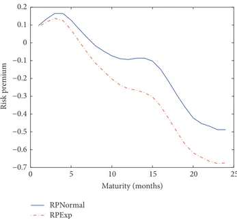
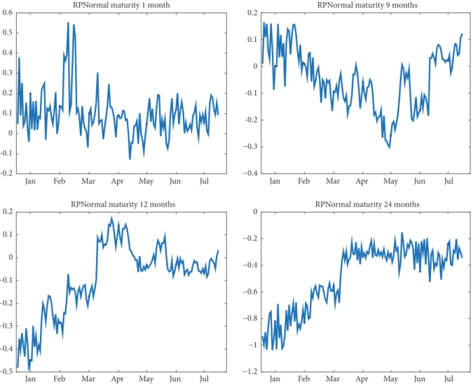
(16) 8. Chapter 1: Introduction. convenience yield. We assume that the spot price follows a jump-diffusion process because of the abrupt changes that happen in the commodity market (see Deng [27] among others) and the convenience yield follows a diffusion process, as commonly found in the literature; see Schwartz [73], and Yan [86]. The main contribution of this chapter is twofold. First, we obtain some results that allow us to estimate the functions of a two-factor risk-neutral jump-diffusion commodity model directly from the spot and futures prices in the market. Finally, we show the effect of considering jumps in the commodity spot price. In Chapter 4, we also consider a jump-diffusion process for the spot price, but we assume different jump size distributions. In this case, our goal is to understand the role of the jump and its distribution. Then, we price natural gas futures and futures options with the different jump size distributions. As futures prices are considered an important information source of expected spot prices, financial investors use them to hedge against the risk of commodity price. Therefore, we also analyze the natural gas futures risk premium. In the literature, empirical evidence of seasonality has been widely shown for different commodity markets such as electricity, natural gas, soybean and so on; see Arismendi et al. [3], Back and Prokopczuk [4], Cartea and Figueroa [20], Kyriakou et al. [53], Li et al. [55], and Lucia and Schwartz [56]. In order to take into account this fact, in Chapter 5, we add a multiplicative seasonal component in the model. In particular, we assume a seasonal deterministic function which is a trigonometric polynomial whose parameters are approximated by means of the nonlinear least square method. As in this case, a closed-form solution is not known, we prove some results to estimate the risk-neutral functions of the model using data from the markets. Finally, we show how to implement this approach using natural gas data and we analyze the role of the seasonality in the futures, futures options and futures risk premia..

(17) Chapter 2. Introducción En la actualidad los mercados de materias primas son muy relevantes por diferentes motivos. Por un lado, son fundamentales para las empresas que buscan cubrirse del riesgo de los posibles cambios de los precios de las materias primas. Por otro lado, son muy atractivos, también, para los inversores financieros que los utilizan para diversificar sus inversiones, véase Back y Prokopczuk [4]. Además, la importancia de estos mercados ha aumentado considerablemente desde el comienzo de este siglo, convirtiéndose en un tema de investigación muy actual. Los precios de las materias primas han experimentado variaciones recientemente, que han sido bastante anómalas por diferentes motivos. Desde la primera década del año 2000, estos precios han reflejado, en general, una tendencia creciente. De hecho, entre el año 2002 y mediados del año 2008 este crecimiento, tanto en magnitud como en duración, ha sido el más importante en décadas. Posteriormente, con el comienzo de la reciente crisis global, los precios comenzaron a disminuir y este fenómeno afectó a un gran número de materias primas. Sin embargo, desde el año 2009, y especialmente desde el verano de 2010, los precios en general comenzaron de nuevo a aumentar. Durante estos años los precios de las materias primas han experimentado también una gran volatilidad. Este fenómeno coincide, también, con una serie de cambios importantes que han tenido lugar en las bases de los mercados. Por ejemplo, tanto la oferta como la demanda de los paı́ses emergentes han crecido de manera considerable en poco tiempo. Por otro lado, el objetivo general de reducir el uso de combustibles fósiles como fuente de energı́a y el debate sobre el cambio climático y su relación con la agricultura han tenido también un importante efecto sobre la evolución de los precios de las materias primas. Sin embargo, estos factores no son suficientes para explicar el comportamiento más reciente de estos precios. Ası́, un factor adicional es la mayor presencia de inversores financieros en estos mercados, los cuales buscan diversificar sus inversiones más allá de los tradicionales activos financieros. Este fenómeno se conoce como financialization de los mercados y su relevancia ha aumentado considerablemente desde el año 2004, como se puede deducir a partir del elevado crecimiento experimentado por el número de inversiones financieras realizadas en los 9.

(18) 10. Chapter 2: Introducción. mercados de materias primas desde dicho año. Este factor es muy importante porque la actividad de estos inversores financieros puede mover los precios de las materias primas lejos de los niveles que establecen las leyes de la oferta y la demanda. Los inversores financieros toman decisiones de negocio que no se basan totalmente en las caracterı́sticas propias de las materias primas, sino más bien en aspectos relacionados con la composición de sus carteras y la tendencia seguida por los mercados en un determinado momento. Estos comportamientos pueden, incluso, tener efectos negativos tanto sobre los consumidores como sobre los productores de las materias primas.. 2.1 Los mercados de materias primas La negociación de las materias primas en los mercados es bastante limitada ya que sus participantes buscan, normalmente, una exposición financiera a los movimientos de los precios de la materia prima subyacente más que a la propia materia prima. Por tanto, tal y como señalan Back y Prokopczuk [4], la negociación y la fijación de los precios de las materias primas tiene lugar en los mercados de futuros de dichos productos. Los derivados sobre materias primas se negocian tanto en mercados organizados como en mercados no organizados u over the counter, utilizando normalmente una institución financiera como intermediario. En los mercados de futuros se negocian productos estandarizados, claramente definidos, que ofrecen una gran liquidez, transparencia y reducen el riesgo de posible impago. Sin embargo, el número y variedad de este tipo de contratos estandarizados es bastante limitado y no siempre proporcionan una cobertura perfecta a sus participantes. En los mercados no organizados los agentes pueden negociar contratos más amplios que los futuros estandarizados existentes y adaptarlos a sus preferencias y necesidades. Sin embargo, a pesar de que estos contratos ofrecen mayor libertad, y en general menores costes potenciales de negociación, pueden incurrir en mayor riesgo de impago para ambas partes, pues no suelen utilizar los servicios de las cámaras de compensación. De hecho, todavı́a actualmente, los mercados no organizados suelen ser bastante opacos en todas las partes del mundo. En Estados Unidos los mercados más conocidos son aquellos pertenecientes al CME Group, el cual surgió después de la fusión del Chicago Mercantil Exchange (CME) y el Chicago Board of Trade en 2006. De hecho, el New York Mercantil Exchange (NYMEX) también pertenece a este grupo y es uno de los mercados más activos a nivel mundial. Las materias primas negociadas en los mercados son muy diversas pero pueden agruparse en cuatro grandes categorı́as: • Metales. Este tipo de materias primas son probablemente las más negociadas y pueden, a su vez, dividirse en otras categorı́as, como por ejemplo metales preciosos (oro, plata,. . . ), metales no preciosos (cobre, aluminio,. . . ), acero, etc • Energı́a. Estas materias primas son las más influyentes e incluyen petróleo, gas natural, carbón, etc..

(19) 2.2 Los precios al contado y los futuros. 11. • Productos agrı́colas. En este grupo se incluye el algodón, el cacao, el azúcar, el zumo de naranja, etc. • Ganaderı́a y carne, como por ejemplo el ganado vacuno, porcino, etc. Los futuros son una forma muy conocida de invertir en materias primas. Estos contratos se realizan en un mercado organizado entre dos partes con el objetivo de comprar (o vender) una cantidad establecida de una materia prima determinada a un precio fijo y en una fecha estipulada. Otra posible forma de invertir en materias primas es a través de opciones. Las opciones proporcionan una mayor flexibilidad a los inversores que los futuros, ya que están diseñadas para ofrecer el derecho (no la obligación) de comprar (o vender) una determinada materia prima o contrato a un determinado precio y en una fecha futura establecida de antemano, véase Cummins y Murphy [26]. En los mercados financieros de materias primas participan, fundamentalmente, dos tipos de participantes: • Los inversores, que compran y venden contratos para protegerse de los movimientos que pueden experimentar los precios de las materias primas. Por tanto, buscan evitar riesgos. • Los especuladores, que tratan de enriquecerse analizando el comportamiento de los mercados de materias primas, adelantándose a los posibles movimientos en sus precios y comprando y vendiendo los diferentes contratos en circulación.. 2.2 Los precios al contado y los futuros En los mercados de materias primas es interesante conocer la estructura temporal de los precios de los futuros sobre materias primas o curva de futuros, la cual es la relación existente entre los precios de los futuros para diferentes vencimientos en un determinado momento, véase Lautier [54]. De hecho, los cambios en la pendiente de la curva de futuros tienen importantes consecuencias sobre las decisiones de inversión y gestión de riesgo, y han sido el centro de numerosos trabajos de investigación, véanse Acharya et al. [1], Bessembinder y Lemmon [13] y Geman y Ohana [35]. Una curva de futuros se dice que tiene pendiente creciente cuando los precios de los futuros son mayores que los precios al contado. En esta situación se considera que el mercado está en contango. Por el contario, cuando el precio de los futuros está por debajo del precio al contado, la curva de futuros tiene pendiente decreciente y se dice que el mercado está en backwardation. Sin embargo, lo más habitual es que estas curvas presenten tramos crecientes y decrecientes, incluso su forma suele variar a lo largo del tiempo, véase por ejemplo Hambur y Stenner [42]. La forma de la estructura temporal de los precios de los futuros ha venido explicada tradicionalmente por dos corrientes: la teorı́a de inventarios, la cual comenzó con Brennan [16] y Kaldor [50] entre otros, y la literatura sobre la presión de cobertura o hedging pressure, de la cual fueron pioneros Hicks [45] y Keynes [51]..

(20) 12. Chapter 2: Introducción. La teorı́a de inventarios se centra en el beneficio global que reporta poseer la materia prima fı́sicamente ası́ como de algunos aspectos relacionados con su almacenamiento. Poseer la materia prima proporciona ciertos beneficios pero también conlleva ciertos costes. Por tanto, el rendimiento de conveniencia (neto) se define como la diferencia entre el rendimiento de conveniencia bruto menos el coste de poseer fı́sicamente el bien, como por ejemplo los costes de almacenamiento, transporte, etc. En lı́nea con esta teorı́a, existe una relación entre el precio al contado y el precio de los correspondientes futuros. Si los beneficios de poseer las materias primas (rendimiento de conveniencia) son mayores que sus costes financieros (tipo de interés), la curva de futuros estará en backwardation, sin embargo, si los costes financieros son superiores al rendimiento de conveniencia, entonces la curva estará en contango, véase Back y Prokopczuk [4] para más información. La posesión de la materia prima permite también a los productores cubrir cambios inesperados de la demanda, periodos temporales de escasez de oferta y asegurarse el proceso de producción véase Kwok [52]. Por tanto, a partir de argumentos relacionados con la oferta y la demanda se establece también una relación negativa entre el nivel de los inventarios y el precio, véase Back y Prokopczuk [4]. Ası́, si el nivel de los inventarios es elevado, la curva de futuros estará en contango y, si el nivel de los inventarios es bajo, la curva de futuros estará en backwardation. Por el contrario, la teorı́a de la hedging pressure se centra en la prima de riesgo. Esta corriente considera que el precio de los futuros es la suma del precio al contado esperado más una prima de riesgo. La teorı́a de la normal backwardation propuesta por Keynes [51] se basa en la hipótesis general de que los productores, normalmente, toman posiciones cortas en los contratos de futuros porque desean asegurarse cierto precio en el momento de la entrega de la materia prima. Este contrato proporciona a los productores una forma de cubrirse del riesgo de descenso del precio al contado. Por tanto, los productores están dispuestos a pagar una prima de riesgo que les cubra su exposición a variaciones del precio de la materia prima. Por otro lado, los consumidores también pueden estar interesados en protegerse de posibles subidas del precio. Por tanto, tomarán una posición larga en los correspondientes contratos de futuros. Si la actividad de cobertura de los productores de una determinada materia prima es mayor que la actividad de los consumidores, el precio de los futuros será menor que el precio al contado esperado, y el precio de los futuros será un estimador sesgado por defecto del precio al contado esperado, véase Back y Prokopczuk [4]. Esta situación inducirá a los especuladores a equilibrar el mercado tomando la posición contraria, es decir, una posición larga. Sin embargo, esta situación no siempre es válida. Si la actividad de cobertura de los consumidores es mayor que la de los productores, habrá un exceso de participantes en el mercado buscando entrar en una posición larga y, por tanto, el precio del futuro será menor que el precio al contado esperado en un momento futuro. En este caso, los especuladores deberán ser de alguna manera recompensados por tomar una posición corta en el futuro y ası́ equilibrar el mercado. Por tanto, los precios de los futuros pueden incluir una prima positiva o negativa dependiendo de la posición neta de los coberturistas para cada materia prima y del instante de tiempo considerado, véanse Cootner [25] y Hambur y Stenner [42]. En este sentido, Hambur y Stenner [42] definen la prima de riesgo como el rendimiento que los especuladores esperan obtener como compensación.

(21) 2.3 Modelos de valoración. 13. por comprar y/o vender contratos de futuros sobre materias primas. El papel que desempeña la prima de riesgo en los diferentes mercados de materias primas ha sido ampliamente analizado, véanse por ejemplo Acharya et al. [1], Basu y Miffre [8] y Ronn y Wimschulte [69].. 2.3 Modelos de valoración En los últimos años se han propuesto diferentes modelos relacionados con la valoración de derivados de materias primas. En este tipo de modelos, en primer lugar, se deben establecer las variables de estado y su dinámica, todo ello buscando un equilibrio entre que el modelo sea sencillo de implementar y que sea capaz de capturar adecuadamente las propiedades de los precios. Evidentemente, el precio al contado de la materia prima deberı́a ser una de las variables a tener en cuenta para valorar futuros. Muchos modelos describen la dinámica de esta variable mediante un proceso estocástico y utilizan argumentos de no arbitraje para la valoración del derivado, véase Schwartz [73]. Debido a la relación entre la demanda y la oferta se suele considerar que el precio al contado tiene un comportamiento de reversión a la media. Por ejemplo, Bessembinder et al. [12] muestran una fuerte evidencia de reversión a la media en los mercados de materias primas, sin embargo, Brooks y Prokopczuk [18] afirman que la reversión a la media no se mantiene cuando el modelo presenta saltos y volatilidad estocástica. De hecho, en la literatura se han propuesto diferentes tipos de dinámicas: Schwartz [73] supone que la reversión a la media es constante mientras que Schwartz y Smith [74] consideran una media a largo plazo estocástica. Brennan y Schwartz [17] proponen un modelo de un factor donde el rendimiento de conveniencia se describe mediante una función determinista del precio al contado. Sin embargo, los modelos unifactoriales no son consistentes con la observación empı́rica, ya que proporcionan precios de futuros que están perfectamente correlacionados. Por tanto, parece que estos modelos no son capaces de reflejar la dinámica de los precios de los futuros. Gibson y Schwartz [36] introducen un modelo con procesos de difusión conjuntos del precio al contado y el rendimiento de conveniencia; más concretamente, consideran que el precio al contado sigue un movimiento Browniano geométrico y el rendimiento de conveniencia está descrito mediante un proceso Ornstein-Ulhenbeck. Como el rendimiento de conveniencia no es observable en el mercado, Gibson y Schwartz [36] proponen una proxy para esta variable. Schwartz [73] considera un modelo de tres factores con un factor adicional, el tipo de interés, que sigue un proceso de difusión. Posteriormente, Miltersen y Schwartz [59] también proponen un modelo de tres factores para valorar futuros de materias primas y opciones de futuros. Recientemente, Schöne y Spinler [72] consideran un modelo de difusión afı́n con volatilidad estocástica para valorar también futuros y opciones. Muchas materias primas se caracterizan por presentar excepcionalmente cambios bruscos en los precios en el mercado, como consecuencia de fallos en la producción o el transporte, de las condiciones climáticas, en el caso de materias primas agrı́colas, o de sucesos macroeconómicos.

(22) 14. Chapter 2: Introducción. inesperados entre otras razones. En la literatura, con el fin de tener en cuenta estos cambios bruscos en el precio de las materias primas, se añade un término de salto en el proceso estocástico. Por ejemplo, Hilliard y Reis [46] proponen un modelo que permite saltos en el proceso del precio al contado, en particular, suponen que este precio sigue un proceso de difusión con saltos. Yan [86] considera un modelo de valoración de derivados de materias primas con saltos en el precio al contado y la volatilidad. Schmitz et al. [71], en el caso de las materias primas agrı́colas, suponen que la volatilidad es un proceso estocástico con saltos, y analizan su efecto en los precios de las opciones. Hilliard y Hilliard [47] usan, para describir el precio al contado, un movimiento Browniano geométrico con un término de salto y, para el tipo de interés y el rendimiento de conveniencia, procesos de difusión con reversión a la media, todo ello para valorar precios de opciones del oro y el cobre. Finalmente, es bien conocido que la oferta y la demanda de muchas materias primas presentan ciclos estacionales. En particular, las agrı́colas y la mayorı́a de las energéticas tienen un patrón estacional en sus precios. Por un lado, la oferta de las materias primas agrı́colas depende del clima el cual afecta a la producción. Por otro lado, la demanda de energı́a es mayor durante las estaciones frı́as. Por tanto, los precios son más altos durante estas estaciones que en el periodo cálido. Por ejemplo, Sørensen [75] muestra el patrón estacional que presentan productos agrı́colas como la soja, el maı́z y el trigo, y Manoliu y Tompaidis [57] y Paschke y Prokopczuk [63] encuentran un fuerte efecto estacional en algunas materias primas de la energı́a como el gas natural, el petróleo o la gasolina. Cartea y Figueroa [20], Li et al. [55] y Lucia y Schwartz [56] consideran estacionalidad en mercados de la electricidad, Garcı́a Mirantes et al. [34] en los del gas natural, Kyriakou et al. [53] en los del petróleo y Back y Prokopczuk [4] en mercados de la soja, el maı́z, el petróleo y el gas natural. Arismendi et al. [3] analizan la importancia de la estacionalidad en la volatilidad a la hora de valorar opciones. Mu [60] muestra cómo afecta el clima a la volatilidad del precio del gas natural y que presenta un fuerte patrón estacional. Geman y Ohana [35] y Suenaga et al. [79] encuentran que la volatilidad del precio de gas natural es más alta durante el invierno que durante el verano. Sørensen [75] incluye una componente estacional determinista en el modelo para describir las variaciones estacionales en el precio de la materia prima. Más concretamente, supone que el logaritmo del precio al contado es la suma de una función trigonométrica determinista y dos factores latentes. De hecho, encuentra una fuerte evidencia de estacionalidad en el precio de la soja, el maı́z y el trigo. Considerar polinomios trigonométricos en la componente estacional del modelo tiene algunas ventajas, como que las funciones son continuas en el tiempo y que para su descripción son necesarios pocos parámetros. En otros casos, se consideran variables estacionales dummy para su modelización, véanse por ejemplo Benth et al. [11] y Lucia y Schwartz [56]. Este enfoque es muy flexible, pero generalmente requiere de un gran número de parámetros. Garcı́a Mirantes et al. [34] proponen como factores estacionales componentes trigonométricos generados por procesos estocásticos..

(23) 2.4 Metodologı́a. 15. 2.4 Metodologı́a En los modelos de valoración propuestos en este trabajo se utilizan procesos de difusión y de difusión con saltos. Además, añadimos una componente estacional en el precio al contado de la materia prima, y analizamos el papel que tienen los saltos y la componente estacional a la hora de valorar futuros y opciones. Para desarrollar esta investigación, utilizamos la siguiente metodologı́a. La herramienta fundamental en los modelos de valoración financiera es el cálculo estocástico. En este contexto, consideramos un espacio de probabilidad filtrado completo donde describimos la dinámica de las variables de estado mediante procesos estocásticos. Más concretamente, utilizamos procesos de difusión y difusión con saltos mediante un proceso Browniano y un término de salto. Este término es modelizado con un proceso de Poisson con su correspondiente intensidad de salto y los tamaños de salto vienen determinados mediante variables aleatorias que siguen una distribución de probabilidad concreta (normal o exponencial). Además, utilizamos la regla del producto de Ito, ası́ como el Lema de Ito del cálculo estocástico, véanse Applebaum [2], Cont y Tankov [23], Øksendal [62], Protter [67] y Shreve [76] para más detalle. A lo largo del trabajo utilizamos las notaciones diferencial e integral de los procesos estocásticos de difusión y saltos. Para valorar derivados de materias primas consideramos el argumento de no arbitraje, es decir, hacemos una transformación de la medida fı́sica a la neutral al riesgo, mediante el cambio de medida de tipo Girsanov, véanse Bremaud [15] y Shreve [76]. Entonces, expresamos los procesos estocásticos bajo esta medida martingala equivalente. Cuando consideramos procesos de difusión con saltos, debemos tener en cuenta que la medida neutral al riesgo no es única, es decir, el mercado no es completo. Un paso previo a la valoración de derivados de materias primas es la estimación. En este trabajo, utilizamos la estimación paramétrica con el método de mı́nimos cuadrados no lineales, véanse Benth et al. [11], Lucia y Schwartz [56] y Stoer y Bulirsch [78], para obtener simultáneamente todos los parámetros del polinomio trigonométrico de Fourier que aproxima la componente estacional del precio de la materia prima. En lo que respecta al resto de las funciones de los procesos neutrales al riesgo, las estimamos utilizando técnicas no paramétricas, evitando de esta forma restricciones arbitrarias en las funciones. En particular, utilizamos el estimador de NadarayaWatson con el núcleo Gaussiano para las funciones peso, véanse Figà-Talamanca y Roncoroni [32], Fusai y Roncoroni [33], Härdle [43] y Härdle et al. [44], porque este procedimiento es flexible y permite no linealidades en la tendencia, la volatilidad y la intensidad del salto. Con el propósito de ilustrar el proceso de implementación del enfoque propuesto, utilizamos una materia prima energética: el gas natural. Esta materia prima y sus correspondientes contratos (futuros y opciones) son muy lı́quidos y se negocian activamente en el mercado, véase Cummins y Murphy [26]. El precio al contado del gas natural Henry Hub fue obtenido de la US Energy Information Administration del US Department of Energy (EIA database). Los precios diarios de los futuros del gas natural con vencimientos cortos (hasta 4 meses) fueron también obtenidos de la base de datos EIA, y los precios con vencimientos más largos (hasta 44 meses) de la plataforma.

(24) 16. Chapter 2: Introducción. Quandl. Los datos los hemos dividido en dos grupos: el periodo de estimación, que se utiliza precisamente para realizar la estimación de las funciones y parámetros, y un periodo de tiempo de predicción, que es una muestra más reciente y que es donde se valoran los derivados. Finalmente, como en este trabajo utilizamos estimación no paramétrica, no es posible obtener una forma cerrada de la solución. En estos casos, se puede calcular el precio del derivados mediante dos procedimientos: resolviendo numéricamente la ecuación en derivadas parciales integrodiferencial o con el método de Monte Carlo, el cual calcula una aproximación al precio del derivado mediante la esperanza condicionada de la condición final del derivado. Ambas técnicas están relacionadas por medio del Teorema de Feynman-Kac, véanse Pascucci [64] y Shreve [76]. En esta investigación, usamos el método de Monte Carlo generando un gran número de simulaciones del precio al contado subyacente bajo la medida neutral al riesgo. Este método es ampliamente utilizado por investigadores y profesionales de los mercados, especialmente para modelos multifactoriales, debido a su sencillez, véanse Glasserman [37] y Wilmott [84].. 2.5 Contribuciones En la literatura es muy habitual utilizar modelos afines para valorar derivados de materias primas, por su sencillez y adaptabilidad. Para poder obtener una forma cerrada del precio del derivado, se suelen considerar funciones paramétricas sencillas. De hecho, en la mayorı́a de los casos, los precios de riesgo del mercado se consideran constantes. Entonces, las funciones de los procesos bajo la medida neutral al riesgo se estiman a partir de las observaciones de los precios del derivado. Por ejemplo, Gibson y Schwartz [36], Schwartz [73] y Cortazar et al. [24] consideran modelos afines con uno, dos o tres factores, y obtienen una forma cerrada de la solución para el precio del derivado. Sin embargo, estos autores no introducen saltos ni estacionalidad en sus modelos. Además, no hay ninguna evidencia empı́rica de que los modelos afines sean mejores para valorar derivados de materias primas. Si consideramos otras dinámicas más realistas para las variables de estado, no se suele conocer una forma cerrada de la solución. Entonces, los precios de riesgo del mercado o las funciones de los procesos neutrales al riesgo no se pueden estimar, porque no son observables. De hecho, este problema es una de las cuestiones abiertas en la valoración de derivados de materias primas, y es el principal objetivo de esta tesis. Ası́ pues, para resolver este problema, proponemos un nuevo enfoque para estimar las funciones de los procesos neutrales al riesgo del modelo a partir de los datos del mercado, incluso cuando no se conoce una expresión de la solución. Es decir, diseñamos nuevas técnicas de estimación para diferentes comportamientos del precio al contado de la materia prima en el mercado. Además, para ilustrar cómo implementar estas técnicas, utilizamos futuros del gas natural negociados en el NYMEX. En los diferentes capı́tulos de esta tesis mostramos nuestras principales contribuciones. En el Capı́tulo 3 consideramos un modelo de dos factores de difusión con saltos cuyas variables son el precio al contado y el rendimiento de conveniencia. Suponemos que el precio al contado sigue.

(25) 2.5 Contribuciones. 17. un proceso de difusión con saltos, para que recoja los cambios bruscos que se producen en los mercados de materias primas (véase Deng [27], entre otros), y el rendimiento de conveniencia sigue un proceso de difusión, como es habitual en la literatura, véanse Schwartz [73] y Yan [86]. La principal contribución de este capı́tulo es doble. En primer lugar, obtenemos resultados que nos permiten estimar las funciones de un modelo de dos factores de difusión con saltos directamente a partir de los precios de los futuros. Finalmente, mostramos el efecto de considerar saltos en el precio al contado sobre los precios de futuros. En el Capı́tulo 4 también consideramos un proceso de difusión con saltos para el precio al contado, pero suponemos diferentes distribuciones para los tamaños de salto. En este caso, nuestro objetivo es analizar el papel que juega dicha distribución en el modelo y, para ello, valoramos futuros del gas natural y opciones de futuros, con diferentes distribuciones del salto. Los inversores financieros consideran los precios de los futuros como una fuente de información sobre el precio esperado de la materia prima, y lo utilizan para diseñar sus estrategias de cobertura del riesgo. En este capı́tulo analizamos la prima de riesgo de los futuros de materias primas. Diferentes investigadores han mostrado evidencia empı́rica de estacionalidad en diversos mercados de materias primas como la electricidad, el gas natural, la soja, etc, véanse Arismendi et al. [3], Back y Prokopczuk [4], Cartea y Figueroa [20], Kyriakou et al. [53], Li et al. [55] y Lucia y Schwartz [56]. Con el fin de tener en cuenta este hecho, en el Capı́tulo 5 añadimos una componente estacional multiplicativa en el modelo previo. En particular, consideramos una función estacional determinista mediante un polinomio trigonométrico, cuyos parámetros son aproximados mediante el método de mı́nimos cuadrados no lineal. Como en este caso no existe una forma cerrada de la solución, probamos resultados para estimar las funciones de los procesos neutrales al riesgo usando datos del mercado. Finalmente, mostramos cómo implementar estas técnicas utilizando datos de los futuros del gas natural y analizamos el papel de la estacionalidad en los precios de los futuros, las opciones sobre futuros y las primas de riesgo de los futuros..

(26)

(27) Chapter 3. A new technique to estimate the risk-neutral processes in jump-diffusion commodity futures models. [This chapter has been previously published (jointly with Lourdes Gómez-Valle and Julia Martı́nezRodrı́guez) in Journal of Computational and Applied Mathematics, vol. 309, pp. 435-441, 2017.]. 19.

(28)

(29) Journal of Computational and Applied Mathematics 309 (2017) 435–441. Contents lists available at ScienceDirect. Journal of Computational and Applied Mathematics journal homepage: www.elsevier.com/locate/cam. A new technique to estimate the risk-neutral processes in jump–diffusion commodity futures models L. Gómez-Valle, Z. Habibilashkary, J. Martínez-Rodríguez ∗ Departamento de Economía Aplicada, Facultad de Ciencias Económicas y Empresariales, Universidad de Valladolid, Avenida del Valle de Esgueva 6, 47011, Valladolid, Spain. article. info. Article history: Received 19 October 2015 Received in revised form 18 December 2015 Keywords: Commodity futures Jump–diffusion stochastic processes Risk-neutral measure Numerical differentiation Nonparametric estimation. abstract In order to price commodity derivatives, it is necessary to estimate the market prices of risk as well as the functions of the stochastic processes of the factors in the model. However, the estimation of the market prices of risk is an open question in the jump–diffusion derivative literature when a closed-form solution is not known. In this paper, we propose a novel approach for estimating the functions of the risk-neutral processes directly from market data. Moreover, this new approach avoids the estimation of the physical drift as well as the market prices of risk in order to price commodity futures. More precisely, we obtain some results that relate the risk-neutral drifts, volatilities and parameters of the jump amplitude distributions with market data. Finally, we examine the accuracy of the proposed method with NYMEX (New York Mercantile Exchange) data and we show the benefits of using jump processes for modelling the commodity price dynamics in commodity futures models. © 2016 Elsevier B.V. All rights reserved.. 1. Introduction The behaviour of many commodity futures has become highly unusual over the past decades. Prices have experienced significant run-ups, and the nature of their fluctuations has changed considerably. This is partly due to financial firms with no inherent exposure to the commodities have adopted strategies of portfolio diversification into commodity futures markets as an asset class, see [1]. However, energy commodities are different from financial assets such as equity and fixed-income securities. For example, changes in market expectations, or even unanticipated macroeconomic developments may cause sudden jumps in energy prices, see [2]. Therefore, traditional modelling techniques are not directly applicable. In order to price commodity derivatives, the empirical features of the commodity prices need to be considered. First, the spot price and other factors were assumed to follow diffusion processes. For example, Gibson and Schwartz [3] assumed that the spot price and the convenience yield were mean-reverting diffusion processes. Then, Schwartz [4] reviewed one and two-factor models and developed a three-factor mean-reverting diffusion model. Later, Miltersen and Schwartz [5] also considered a three-factor model in order to price commodity futures and futures options. More recently, in the literature, jump–diffusion models have been considered because there are numerous empirical studies which show that commodity prices exhibit jumps, [6,7] and so on. Hilliard and Reis [8] considered a three-factor model where the spot price follows a jump–diffusion stochastic process. Yan [9] extended existing commodity valuation models to allow for stochastic volatility and simultaneous jumps in the spot price and volatility. Hilliard and Hilliard [10] used the standard geometric Brownian. ∗. Corresponding author. E-mail addresses: lourdes@eco.uva.es (L. Gómez-Valle), ziba.habibilashkary@alumnos.uva.es (Z. Habibilashkary), julia@eco.uva.es (J. Martínez-Rodríguez). http://dx.doi.org/10.1016/j.cam.2015.12.028 0377-0427/© 2016 Elsevier B.V. All rights reserved..

(30) 436. L. Gómez-Valle et al. / Journal of Computational and Applied Mathematics 309 (2017) 435–441. motion augmented by jumps to describe the underlying spot and mean-reverting diffusions for the interest rate and convenience yield state variables for gold and copper prices. In this paper, we consider a two-factor jump–diffusion commodity model, where one of the factors is the commodity spot price. In the commodity literature, it is very common to use affine models for its simplicity and tractability. They select the simple parametric functions for the model in order to obtain a closed-form solution for the pricing problem. This is mainly important for the market prices of risk, which are assumed to be constant in most of the cases. Then, all the functions can be easily estimated and the commodity derivatives priced. However, there is not any empirical evidence either consensus about affine models are the best models to price commodity futures. Furthermore, the market prices of risk are not observed in the markets. If we considered other more realistic functions for the state variables or the market prices of risk or even a nonparametric approach, then, the model would not be affine anymore, a closed-form solution could not be obtained and therefore, the estimation of the market prices of risk would not be possible. In fact, this last problem is an open question in the jump–diffusion commodity literature. The main contribution of this paper is twofold. First, we obtain some results that allow us to estimate the risk-neutral functions of a two-factor jump–diffusion commodity model directly from commodity spot and futures data on the markets. Therefore, we can obtain a closed-form solution or a numerical approximation for the pricing problem without estimating the market prices of risk, which are not observed and possible to estimate when a closed-form solution is not known. Second, we show the effect of considering jumps in the commodity spot price over the futures prices. We use NYMEX data and a nonparametric approach to estimate the whole functions of our two-factor model. We think that using a nonparametric approach is more realistic than using an affine model. The remaining of the paper is arranged as follows. In Section 2, we present a two-factor jump–diffusion model to price commodity futures. In Section 3, we prove some results which allow us to estimate the risk-neutral drift, jump intensity and parameters of the distribution of the jump amplitude from spot commodity price and futures data. In Section 4, we estimate our two-factor jump–diffusion model with NYMEX data by means of a nonparametric approach, we price commodity futures and we show its supremacy over a diffusion model. Section 5 concludes. 2. The valuation model In this section, we present a two-factor commodity futures model. The first factor is the spot price S, and the second factor is δ , which could be, for example, the instantaneous convenience yield or the volatility among other possible variables. Let (Ω , F , P ) be a probability space equipped with a filtration F satisfying the usual conditions, see [11,12] or [13]. The factors of the model are assumed to follow this joint jump–diffusion stochastic process: dS (t ) = µS (S (t ), δ(t ))dt + σS (S (t ), δ(t ))dWS (t ) + J (S (t ), δ(t ), Y (t ))dN (t ),. (1). dδ(t ) = µδ (S (t ), δ(t ))dt + σδ (S (t ), δ(t ))dWδ (t ),. (2). where µS and µδ are the drifts, σS and σδ the volatilities. The jump amplitude J is a function of the two factors and Y which is a random variable with probability distribution Π . Moreover, WS and Wδ are Wiener processes and N represents a Poisson process with intensity λ. We assume that the standard Brownian motions are correlated with: Cov(WS , Wδ ) = ρ t . However, WS and Wδ are assumed to be independent of N. We also assume that the jump magnitude and the jump arrival time are uncorrelated with the diffusion parts of the processes. We suppose that the functions µS , µδ , σS , σδ , J , λ and Π satisfy suitable regularity conditions: see [11,14]. Under the above assumptions, a commodity futures price at time t with maturity at time T , t ≤ T , can be expressed as F (t , S , δ; T ) and at maturity it is F (T , S , δ; T ) = S . Finally, we assume that there exists a replicating portfolio for the futures price and then, the futures price can be expressed by F (t , S , δ; T ) = E Q [S (T )|S (t ) = S , δ(t ) = δ],. (3). Q. where E denotes the conditional expectation under the Q measure which is known as the risk-neutral probability measure. The two-factor model (1)–(2) under Q measure is as follows: dS = µS − σS θ WS + λQ EYQ [J ] dt + σS dWSQ + JdÑ Q ,. (4).   dδ = µδ − σδ θ Wδ dt + σδ dWδQ ,. (5). . . where WSQ and WδQ are the Wiener processes under Q and Cov(WSQ , WδQ ) = ρ t. The market prices of risk of Wiener. processes are θ WS (S , δ) and θ Wδ (S , δ), and Ñ Q represents the compensated Poisson process, under Q measure, with intensity λQ (S , δ) = λ(S , δ)θ N (S , δ)..

(31) L. Gómez-Valle et al. / Journal of Computational and Applied Mathematics 309 (2017) 435–441. 437. 3. Exact results and approximations In the literature, researchers have devoted the greatest attention to affine models such as [4,8–10]. One of the main reasons is that a closed-form solution for the commodity futures price is found. Moreover, this fact allows the application of different estimation techniques, like the Kalman Filter or Maximum Likelihood. However, there is neither evidence nor consensus that affine models are the most suitable for pricing futures contracts. In the literature, to the best of our knowledge, there is no approach for estimating the market prices of risk for pricing commodity derivatives with jumps, unless a closed-form solution is known. Bandi and Nguyen [15] and Johannes [14] showed how to estimate the functions of a jump–diffusion process by means of their moment equations for interest rate models. However, this approach does not allow us to estimate the market prices of risk, which are necessary to price commodity derivatives but not observable. In this section, we propose a new approach for estimating the functions of the risk-neutral jump–diffusion stochastic factors of a commodity model directly from market data. Then, we can price futures and the estimation of the market prices of risk can be avoided. Theorem 1. Let F (t , S , δ; T ) be the price of the future (3), and S and δ follow the stochastic processes given by (4) and (5), respectively, then:.   ∂F (t , S , δ; T ) = µS − σS θ WS + λQ EYQ [J ] (T ), ∂T   ∂(SF ) ∂F (t , S , δ; T ) = 2S + σS2 + λQ EYQ [J 2 ] (T ), ∂T ∂T   ∂F ∂(δ F ) (t , S , δ; T ) = δ + S (µδ − σδ θ Wδ ) + ρσS σδ (T ). ∂T ∂T. (6) (7). (8). We prove these results by means of (3). The detailed proof of this theorem can be found in the Appendix. Analogous results, but for diffusion processes, are also shown in [16]. Parallel results for one-factor jump–diffusion interest rate models can be found in [17,18]. In order to implement Theorem 1 we rely on numerical differentiation. We use futures prices at a point that is inside the time interval to approximate the slopes at the boundary of the time domain. This fact allows us to consider futures prices with a high spectrum of maturities for the estimation of the functions of the model. More precisely, we obtain a fourth order approximation to the slopes by the well-known difference formula:. −25g (t ) + 48g (t + ∆) − 36g (t + 2∆) + 16g (t + 3∆) − 3g (t + 4∆) ∂g | = + O(∆4 ). ∂ T T =t 12∆. (9). Finally, it is important to remark that after approximating the slopes in Theorem 1, any parametric or nonparametric technique can be applied to estimate them. In this paper, we use the Nadaraya–Watson nonparametric estimator in order to avoid imposing arbitrary restrictions to the different functions of the model. Suppose a data set consists of N observations, (S1 , δ1 , Z1 ), . . . , (SN , δN , ZN ), where (Si , δi ) are the explanatory variables and Zi is the response variable. We assume a model of the kind Zi = g (Si , δi )+ϵi , where g (S , δ) is an unknown function and ϵi is an error term, representing random errors in the observations or variability from sources not included in the (Si , δi ) observations. The errors ϵi are assumed to be independent and identically distributed with mean 0 and finite variance. The estimate has the closed-form N . ĝ (S , δ) =. wi (S , δ)Zi. i=1 N . , wi (S , δ). i=1. where wi (S , δ) = K. . S −Si hS.   K. δ−δi hδ. . are weight functions (we use the multivariate Gaussian kernel which is also widely. used in the literature) and hS , hδ the bandwidths, see [19]. 4. Empirical application In this section, we show how practitioners can implement the approach in Section 3 for pricing commodity futures in the markets. Moreover, we analyse the effect of adding jumps to the commodity spot price over the futures prices. In this empirical application, we use the commodity spot price and the convenience yield as state variables, which are frequently used in the literature, see for example [3,4]. We assume that the spot price follows a jump–diffusion process, because commodity prices usually suffer from abrupt changes in the markets, see [6]. However, we assume that the convenience yield is a diffusion process because its behaviour is not affected by extreme changes, see for example [9]..

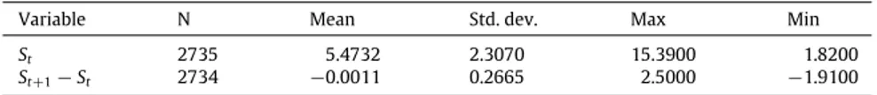
(32) 438. L. Gómez-Valle et al. / Journal of Computational and Applied Mathematics 309 (2017) 435–441 Table 1 Summary of the statistics on the natural gas spot price and its first differences, January 2004–December 2014. Variable. N. Mean. Std. dev.. Max. Min. St St +1 − St. 2735 2734. 5.4732 −0.0011. 2.3070 0.2665. 15.3900 2.5000. −1.9100. 1.8200. For simplicity and tractability and as usual in the literature, we also assume that the distribution of the jump size under. Q measure is known and equal to the distribution under P measure. This means that all risk premium related to the jump. are artificially absorbed by the change in the intensity of the jump from λ under the physical measure to λQ under the riskneutral measure, see [20]. Moreover, we assume in (4) that J (S , δ, Y ) = Y , where Y is a random variable which follows a normal distribution N (0, σY ), see [9,21,22] among others. Therefore, EYQ [Y ] = EY [Y ] = 0. In order to show how the approach in Section 3 can be implemented, we will price natural gas futures with daily data from the NYMEX. Natural gas spot and futures prices were obtained from the Energy Information Administration of the U.S. Department of Energy (E.I.A. database) and Quandl platform. The sample period covers from January 2004 to April 2015. Fig. 1 plots the natural gas spot price data and its first differences. We also consider futures prices with maturities equal to 1, 2, 3, 4, 6, 9, 12, 18, 24, 36 and 44 months. We use data from January 2004 to December 2014 for estimating the riskneutral functions. Table 1 summarizes the in-sample data. We keep data from January to April 2015 as out-of-sample data in order to evaluate the results of our approach. As it is well known in the literature, the convenience yield is not observed in the markets. Then, following [3], we approximate it by the following result. δT −1,T = rT −1,T − 12 ln. F (t , S , δ; T ). . F (t , S , δ; T − 1). . ,. where rT −1,T denotes the T − 1 period ahead annualized one month riskless forward interest rate. We obtain this forward interest rate with two daily T-Bill rates with maturities as close as possible to the futures contracts’ ones in order to compute δ1,2 , the one-month ahead annualized convenience yield. The latter is identified with the instantaneous convenience yield δ0,1 in this study, see [3] for more details. T-Bill rates are obtained from the Federal Reserve h.15 database. First, we obtain the compensated risk-neutral drift of the spot price. We approximate the partial derivative in (6), using numerical differentiation (9), with futures prices with maturities equal to 1, 2, 3 and 4 months. Then, we estimate it by means of the Nadaraya–Watson estimator. Secondly, in order to obtain the risk-neutral jump intensity, we approximate the ∂(SF ) partial derivatives ∂∂ TF |T =t and ∂ T |T =t in (7), using numerical differentiation (9) with spot prices and futures prices with maturities equal to 1, 2, 3 and 4 months. In order to estimate the functions of the stochastic processes of S and δ under the physical measure, we use the following result. Theorem 2. If S and δ solve (1)–(2), then MS1 (S , δ) = lim. ∆t →0. MS2 (S , δ) = lim. ∆t →0. MSk (S , δ) = lim. ∆t →0. Mδ2 (S , δ) = lim. ∆t →0. 1. ∆t 1. ∆t 1. ∆t 1. ∆t. E [S (t + ∆t ) − S (t )|S (t ) = S , δ(t ) = δ] = µS (S , δ) + λ(S , δ)EY [Y ],. (10). E [(S (t + ∆t ) − S (t ))2 |S (t ) = S , δ(t ) = δ] = σS2 (S , δ) + λ(S , δ)EY [Y 2 ],. (11). E [(S (t + ∆t ) − S (t ))k |S (t ) = S , δ(t ) = δ] = λ(S , δ)EY [Y k ],. (12). E [(δ(t + ∆t ) − δ(t ))2 |S (t ) = S , δ(t ) = δ] = σδ2 (S , δ),. (13). E [(S (t + ∆t ) − S (t ))(δ(t + ∆t ) − δ(t ))2 |S (t ) = S , δ(t ) = δ] = ρ(S , δ)σS (S , δ)σδ (S , δ).. (14). 1. Cov(S , δ) = lim. ∆t. ∆t →0. k ≥ 3,. This theorem can be proved with the infinitesimal operator (see [12]), as in [23,24], for diffusion processes, and in [14,15], for jump–diffusion processes. As we have previously assumed, the jump size distribution under Q measure is known and equal to the distribution under P measure and Y ❀ N (0, σY2 ), then EYQ [Y ] = EY [Y ] = 0 and σY2 = EYQ [Y 2 ] = EY [Y 2 ]. Therefore, we estimate σY2 and the volatility of the spot price σS , by means of the moment equations of a jump–diffusion process in Theorem 2, when the jump amplitude follows a normal distribution. More precisely, as Y ❀ N (0, σY2 ), then: EY [Y 2k ] = σY2k. k . (2k − 1),. n =1. EY [Y 2k−1 ] = 0,. k = 1, 2, 3, . . . ..