Perceptron and Random Forest classifiers in
EOG recordings of patients with Ataxia SCA2
Roberto Becerra1, Gonzalo Joya2, Rodolfo Garc´ıa1, Luis Vel´azquez3, Roberto Rodr´ıguez3, and Carmen Pino1
1
Facultad de Inform´atica y Matem´atica, Universidad de Holgu´ın, Cuba
idertator,rodolfo,[email protected] 2
Facultad de Matem´atica y Computaci´on, Universidad de la Havana, Cuba
Departamento de Tecnolog´ıa Electr´onica, Universidad de M´alaga, Espa˜na,
Centre for Research and Rehabilitation of Hereditary Ataxias (CIRAH), Holgu´ın, Cuba
Abstract. In this paper, we compare the performance of two different methods for the task of electrooculogram saccadic points classification in
patients with Ataxia SCA2:Multilayer Perceptrons (MLP) andRandom
Forest. First we segment the recordings of 6 subjects into ranges of sac-cadic and non-sacsac-cadic points as the basis of supervised learning. Then, we randomly select a set of cases based on the velocity profile near each selected point for training and validation purposes using percent split scheme. Obtained results show that both methods have similar perfor-mance in classification matter, and seems to be suitable to solve the problem of saccadic point classification in electrooculographic records from subjects with Ataxia SCA2.
Keywords: eog signals, multilayer perceptron, random forest, saccades, ataxia sca2
1
Introduction
Electrooculography is a common technique for measuring eye movements due its affordability and its accuracy. In the Centre for Research and Rehabilitation of Hereditary Ataxias (CIRAH) of Cuba, this technique is used for monitoring of patients with hereditary ataxias. Specifically, saccadic eye movements have an special interest for the researchers of this disease. This is because many parame-ters calculated from eye movements are affected by the evolution of this disease [1].
a saccade. Currently the identification of these points is performed by manual means by experts in the area or automatically by computational algorithms.
Identification by manual means have drawbacks such as the subjectivity in-troduced by the expert which makes the points selection. This subjectivity gener-ates variability between the identification performed by various of these experts. In the case of signals recorded to sick subjects, the difficulties of manual identi-fication rises due the presence of noises and conditions inherent of the disease.
The way of detecting saccadic points by computational methods is very var-ied and somehow formalized by the taxonomy of Salvucci-Goldberg [3]. Among the methods described by the taxonomy the most common ones are those based on velocity thresholds. These methods have as main drawback that for subjects affected severely by neurological diseases such as Ataxia SCA2, the identification of saccadic points is very inaccurate. Besides there is no consensus in the litera-ture about what value should take the velocity threshold used by these methods. There is a serious lack of research about the other methods proposed in the tax-onomy, but presumably there is a notable difference in the results yielded by them and those yielded by velocity thresholds based methods.
From saccadic points and the corresponding signal channel, is possible to calculate saccadic features such as maximum velocity, latency, duration and the amplitude. These features have proven to be useful in the research of many neurological diseases due the contrast of the behaviour of these features between patients and healtly individuals, as well as between patients of different diseases. For instance, saccadic velocity is significantly slower in subjects with SCA2 than in control subjects or subjects with other ataxias like SCA1 or SCA3 [4]. Also, the calculation of these features supports drug clinical trials and other kind of efforts to improve living conditions of subjects suffering this disease [1].
Latency, duration and amplitude are features very susceptible to the posi-tion of the saccadic points. So, the variability obtained by the methods currently employed have a negative impact on the utility of final data. On the other hand, the variability caused by the currently employed methods has a negative conse-quence on the interpretation of these features by experts, leading to misdiagnosis.
drawbacks present in traditional identification mechanisms.
The rest of this paper is organized as follows: In section 2 we describe the designed experiments and available data. Section 3 is devoted to analize and comment the results. Finally, section 4 summarizes the main conclusions and future work lines.
2
Material and Methods
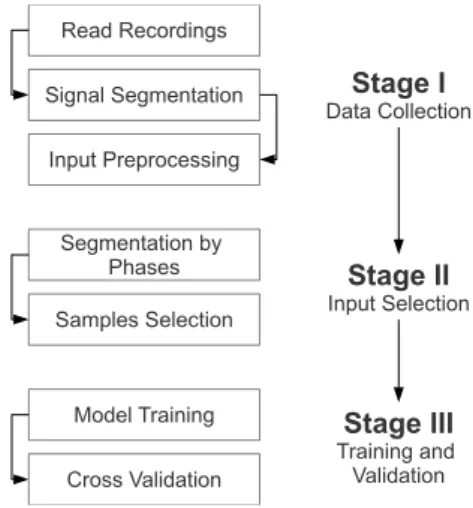
An experiment was designed to apply two machine learning techniques: Mul-tilayer Perceptron (MLP) and Random Forest, to clasify a velocity saccadic pattern dataset. The experiment was separated in several stages as shown in Figure 1. The work performed in each stage is described more deeply in the followings sections.
Fig. 1.Experiment main flow. Each stage are separated in a sequence of ordered steps.
In summary, each stage describes:
Stage I: Provide a set of cases that will conform the population used by the next stage. This population is builded based of EOG segmented data (sac-cadic or non-sac(sac-cadic) created in this stage.
Stage III: Training and validation of both classifiers, using percentage split scheme to separate training data and validation data.
2.1 Data Collection
The data was recorded using the Otoscreen electronystamograph at a sampling rate of 204.8 Hz with a bandwith of 0.02 to 70 Hz (analogic filtering). Specifically, 60 degrees saccadic signals were selected due to it’s difference between healthy and sick subjects. Researchers from the Centre of Research and Rehabilitation of Hereditary Ataxias (CIRAH in spanish) provide us about 30 records of sick subjects, many of them in very bad shape. After the analysis of these records, only six of them meets good quality requirements to train classifiers.
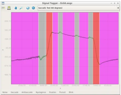
For signal segmentation purposes, a desktop application was developed ca-pable to mark different types of segments as shown in Figure 2.
Fig. 2.Signal editor main window. Pink segments meanfixations, gray segments mean
noise and red segments meansaccades.
Even when the application is capable to tag many ocular events, in selected test only saccades, fixations and noise are relevant. For practical reasons we only need to discriminate saccades and non-saccades, thus, our task becomes a binary classification problem.
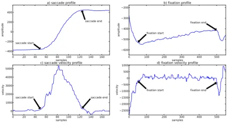
Many classical algorithms used to detect saccadic eye movements use a veloc-ity threshold to set the initial and ending points of a single saccade. Even when they not agreed in a threshold value, there is a consensus about that the main criterion is the velocity. Thus, it seems reasonable to think that the pattern of velocities preceding and after a certain point in the signal determines if they are inside or outside of a certain event as shown in Figure 3.
0 20 40 60 samples80 100 120 140 160 −400 −200 0 200 400 am pli tud e saccade start saccade end
a) saccade profile
0 100 200 samples300 400 500 −600 −500 −400 −300 −200 am pli tud e fixation start fixation end
b) fixation profile
0 20 40 60 80 100 120 140 160 samples 0 1000 2000 3000 4000 5000 ve loc ity
saccade start saccade end
c) saccade velocity profile
0 100 200 300 400 500 samples −2500 −2000 −1500 −1000 −500 0 500 1000 ve loc ity
fixation start fixation end
d) fixation velocity profile
Fig. 3. a) Time signal of a sample saccade, b) Time signal of a sample fixation, c)
Velocity profile of a),d)Velocity profile of b).
The idea for input variables of a single case, was get the pattern of veloc-ities before and after the target point, in a window fashion way. To build the cases population, an sliding window runs through each tagged point in selected records, using this tag as the classification class. If this tag is a saccade we mark the sample as a saccadic point, if the tag is fixation or noise we mark the sample as non-saccadic point.
differentiation noise.
This aggresive filtering is posible because we are interested only in the rela-tionship between the samples in velocity profile, not the waveform itself.
2.2 Input Selection
Once gathered instances population, we proceed to select the samples used for training and validation purposes. Is very important to provide a balanced set of input cases to the classifier in order to achieve better classification performance.
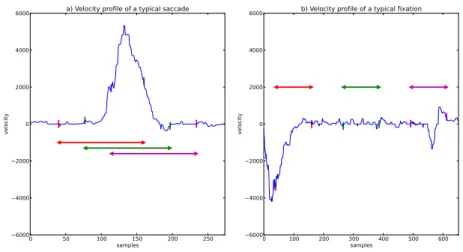
First, the number of cases used for training and validation process selected was 5000. The first half of them was devoted to saccade points and the another half to non saccadic points. The set of non-saccadic points was divided in fixa-tion and noise ponits in equal proporfixa-tions.
0 50 100 samples150 200 250 −6000
−4000 −2000 0 2000 4000 6000
ve
loc
ity
a) Velocity profile of a typical saccade
0 100 200 300samples 400 500 600 −6000
−4000 −2000 0 2000 4000 6000
ve
loc
ity
b) Velocity profile of a typical fixation
Fig. 4. Example of windows of points at beginning, middle and ending of an event.
Red range means a window of a point at beginning of the saccade in a) and fixation in
b).Greenrange means a window of a point at middle of the saccade in a) and fixation
in b).Magenta range means a window of a point at ending of the saccade in a) and
fixation in b).
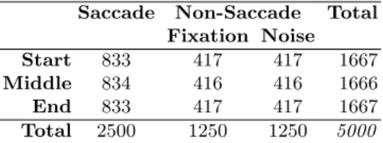
To get even more balanced set of data, was selected the same proportion of beginning, middle and end points of each class. As results of this input selection strategy, the samples count per class lays out in Table 1.
Table 1.Distribution of input samples per zone in the event and per event itself
Saccade Non-Saccade Total Fixation Noise
Start 833 417 417 1667
Middle 834 416 416 1666
End 833 417 417 1667
Total 2500 1250 1250 5000
2.3 Training and Validation
Weka [9] is the software package used for training and validate the selected data.
Previous experiments carried out by the authors indicate that the optimum input features count for the MLP and RF input is of 121 components.
Multilayer Perceptron: MLPs are a kind of feedforward artificial neural net-work which consists in multiples layers of nodes in a directed graph, where each layer is fully connected to the next. Except for the input nodes, each node is a processing element with a nonlinear activation function.
The MLP classifier was trained with a topology of 121 nodes in input layer, 61 sigmoid nodes in the hidden layer and 1 linear node in the output layer. The network use backpropagation as training algorithm with a learning rate of 0.3 and a momentum of 0.2. 500 epochs were used to train this model.
Random Forests: RF is a ensemble of decision trees proposed by Leo Breiman[10]. The idea is based on building a forest of N decision trees, where in each trees we select M input cases in a random way using the same statistical distribution. Breiman in his paper proposes the use of Random Trees in the ensemble. In this type of trees, the split of features in each node is selected randomly from the K best splits.
Weka uses the algorithm proposed by Breiman. In our case we used the de-fault values used in the package. This mean that our model will generate an ensemble of 10 Random Tree. For each tree the random split has 8 features.
The speed and accuracy of RFs make them a very good choice for problems related to computer vision. So we expect very good results from them, because the problem we are treating is in some extent a computer vision problem.
The training process uses 5000 examples distributed as shown in Table 1. The training were evaluated using cross-validation with 5 folds. Finally we test the trained model against 5000 new examples not present in training data.
3
Results
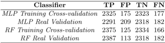
The validation process performed by weka states the following results:
Table 2. Validation results for both classifiers, in training and validation data.TP
are True Positive cases,FPare False Positive cases,TNare True Negative cases and
FNare False Negative cases.
Classifier TP FP TN FN
MLP Training Cross-validation 2325 175 2323 177
MLP Real Validation 2291 209 2318 182
RF Training Cross-validation 2375 125 2334 166
RF Real Validation 2387 113 2318 182
In Table 2Training Cross-validation stands for the results obtained in the training process, andReal Validation stands for the results obtained in the test process (patterns not presented in the training process).
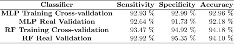
Is a common practice in comparison of several classifiers to use metrics like sensitivity, specificity and accuracy. These metrics are derived from results shown in Table 2 and describe proportions between right and wrong predicted cases.
Sensitivity yields how good the model can predict possitive examples de-scribed by equation 1, in this case saccade points.
Sensitivity= T P
F N+T P ∗100 (1)
Specificityis the proportion on correct prediction on negative cases described by equation 2, in this case non-saccade points.
Specif icity= T N
T N+F P ∗100 (2)
Accuracyis the proportion of right predicted cases, described by equation 3.
Accuracy= T N+T P
Table 3 shows that both methods perform very well and very similar for the proposed task. However, these results also shows that the Random Forest per-forms slightly better than the Multilayer Perceptron.
Table 3.Performance metrics comparison between Multilayer Perceptron and Random Forest classifiers in training and validation data
Classifier Sensitivity Specificity Accuracy MLP Training Cross-validation 92.93 % 92.99 % 92.96 %
MLP Real Validation 92.64 % 91.73 % 92.18 %
RF Training Cross-validation 93.47 % 94.92 % 94.18 %
RF Real Validation 92.92 % 95.35 % 94.10 %
4
Conclusions
This paper presented a comparative between two machine learning techniques (Multilayer Perceptron and Random Forest) to solve saccade and non-saccade point classification problem of EOG signals measured tosubjects with Ataxia SCA2.
The results obtained by the validation of both methods shown an accuracy above 92 percent. So, they are suitable to solve the proposed task without the drawbacks present in traditional methods. Also, this results stated a slightly better performance for Random Forest than Multilayer Perceptron.
The Random Forest classifier could be used to build a pseudo-realtime iden-tification system due its performance in relation to training speed, and for its accuracy.
Acknowledgements
This work has been partially supported by AECID (Spanish Agency for Interna-tional Cooperation and Development, Ministry of Foreign Affairs of Government of Spain) project A2/038418/11.
References
1. Vel´azquez-P´erez, L., Rodr´ıguez-Chanfrau, J., Garc´ıa-Rodr´ıguez, J., S´anchez-Cruz,
Triana, C., Pupo, N., Batista, I., L´opez-Hernandez, O., Polanco, I., Novas, A.: Oral zinc sulphate supplementation for six months in sca2 patients: A randomized,
double-blind, placebo-controlled trial. Neurochemical Research 36 (2011) 1793–
1800
2. Findlay, J.M., Walker, R.: How are saccades generated? Behavioral and Brain
Sciences22(7 1999) 706–713
3. Salvucci, D.D., Goldberg, J.H.: Identifying fixations and saccades in eye-tracking protocols. In: Proceedings of the 2000 symposium on Eye tracking research & applications. ETRA ’00, New York, NY, USA, ACM (2000) 71–78
4. B¨urk, K., Fetter, M., Abele, M., Laccone, F., Brice, A., Dichgans, J., Klockgether,
T.: Autosomal dominant cerebellar ataxia type i: oculomotor abnormalities in
families with sca1, sca2, and sca3. Journal of Neurology246(1999) 789–797
5. Tagluk, M., Sezgin, N., Akin, M.: Estimation of sleep stages by an artificial neural
network employing eeg, emg and eog. Journal of Medical Systems34(2010) 717–
725
6. ¨Oz¸sen, S.: Classification of sleep stages using class-dependent sequential feature
selection and artificial neural network. Neural Computing and Applications (2012) 1–12
7. Jes´us Rubio, J., Ortiz-Rodriguez, F., Mariaca-Gaspar, C., Tovar, J.: A method
for online pattern recognition of abnormal eye movements. Neural Computing and Applications (2011) 1–9
8. Inchingolo, P., Spanio, M.: On the identification and analysis of saccadic eye
movements-A quantitative study of the processing procedures. . . . Engineering, IEEE Transactions on (9) (1985) 683–695
9. Hall, M., Frank, E., Holmes, G.: The WEKA data mining software: an update.
ACM SIGKDD . . .11(1) (2009) 10–18