COMPARISON OF THE CRACK PATTERN IN ACCELERATED CORROSION TESTS AND IN FINITE ELEMENTS SIMULATIONS
B. Sanz1,J. Planas1,J.M. Sancho2
1Departamento de Ciencia de Materiales, E.T.S. de Ingenieros de Caminos, Canales y Puertos, Universidad Polit´ecnica de Madrid, C/ Profesor Aranguren s/n, 28040 Madrid, Espa˜na.
E-mail: [email protected] E-mail: [email protected]
2Departamento de Estructuras de Edificaci´on, E.T.S. de Arquitectura, Universidad Polit´ecnica de Madrid, Avda. Juan de Herrera 4, 28040 Madrid, Espa˜na.
E-mail: [email protected]
ABSTRACT
In this work, the crack pattern obtained in accelerated corrosion tests is compared to the one obtained in numerical simu-lations for reinforced steel concrete samples. In the simusimu-lations, an expansive joint element is used to simulate the oxide layer behaviour together with finite elements with embedded adaptable cohesive crack to simulate the concrete fracture. In parallel, some samples are artificially corroded imposing constant current and after corrosion they are impregnated with resin containing fluorescein to improve the detection of the cracks. In the paper, the main features of the model and the experimental procedure are described and the crack pattern is analysed. A main crack across the concrete cover is easily seen in both cases, but also secondary cracks are observed after treating the concrete surface, in accordance with the model predictions, which gives further support to the ability of the numerical approach to simulate the real cracking processes.
KEY WORDS: Accelerated corrosion tests, Cohesive crack, Finite Elements simulations
1 INTRODUCTION
Corrosion of rebars is an important pathology in rein-forced steel concrete structures. It consists of the gen-eration of an oxide layer at the steel surface that induces internal pressure on the surrounding concrete, due to the greater specific volume of the oxide with respect to the steel, and thus cracks the concrete cover [1, 2, 3].
Focussing on the prediction of the mechanical effects of the oxide expansion over the concrete, a numerical model to simulate the oxide layer behaviour was programmed, assuming that the corrosion depth is given at any speci-fied time [4]. It was calledexpansive joint elementand it has already been presented in previous conferences. That model consists in an interface element with zero ini-tial thickness that incorporates both the expansive and the mechanical behaviour of the oxide, which is char-acterised by its debonding ability, with nearly free slid-ing (very small shear stiffness) and nearly free separa-tion (strongly reduced normal tension stiffness). Con-crete cracking is simulated by finite elements with em-bedded adaptable cohesive cracks [5] that follow the ba-sic cohesive crack model proposed by Hillerborg et al [6].
In parallel, accelerated corrosion tests have been carried out in order to verify the ability of the model to simu-late real processes. The samples are concrete prisms with a steel tube inside simulating a rebar, that are artificially corroded by the imposition of constant current. After cor-rosion, the samples are cut into slices to study the
crack-ing along the bar and they are impregnated under vacuum with resin containing fluorescein to improve the detection of the cracks.
The crack pattern obtained in the tests is compared to the one obtained in numerical simulations of the same pro-cess. In both cases, a main crack is observed from the steel to the concrete surface, but also some secondary cracks and some microcracks can be seen when looking under the microscope or after impregnating the concrete surface with resin and fluorescein, in accordance to the model predictions.
In the paper, the main features of the model and the ex-perimental procedure are described and the crack pattern is analysed.
2 NUMERICAL SIMULATIONS
2.1 Finite element model
In the simulations, finite elements with embedded adapt-able cohesive crack [5] are used to model the concrete cracking. Those elements follow the basic cohesive crack model [6] and they are programmed in C++ within the fi-nite element framework COFE (Continuum Oriented
Fi-nite Elements).
by the authors [4] within the finite element framework COFE. It consists in a four-node element with zero ini-tial thickness and it is defined by the iniini-tial length and the normal direction. The model works assuming elas-tic behaviour, small strain and direct integration at the nodes. The main parameters of the model are the corro-sion depthx(the amount of steel that is transformed into oxide) and a factorβthat indicates the volumetric expan-sion of the oxide respect to the initial steel section and which depends on the ratio of the specific volumes of ox-ide and steel. A sketch of the model is shown in figure 1. It must be remarked that only the part corresponding to the volumetric expansion is considered as expansive joint element and the steel section is kept constant during the calculations, so mechanical equivalence between the element and the real oxide needs to be established. The main equations of the model are detailed in the appendix at the end of the paper.
!x = volumetric expansion expansive joint element
initial steel section fixed contact
steel-joint element real oxide
x = corrosion depth
Figure 1: Sketch of the expansive joint element
2.2 Parameters of the simulations
The samples in the simulations are concrete prisms of 90 mm height and 100 mm width with a 20 mm diam-eter smooth steel bar cast-in, centred with respect to the width, and with a concrete cover equal to the diameter of the bar. The concrete is modelled with elements with embedded adaptable cohesive crack, the steel with linear elastic elements and the oxide with expansive joint ele-ments. The mesh is generated using the pre-post FE mesh processor Gmsh [7]. The elements are constant strain tri-angles.
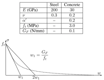
The mechanical properties of steel and concrete were ex-perimentally determined by mechanical tests (compres-sion, brazilian and three point bending tests) [8, 9, 10, 11], so the parameters of the materials in the simulations are the same as the real ones. They are shown in table 1.
Twolinearapproximations for the softening curve have
been used. The first one has a fracture energyGF = 0.1
N/mm (100 N/m), which corresponds to the actual to-tal fracture energy of the material, and, except for the tail, lies well above the actual softening function, as shown in Fig. 2. The second one has a fracture energy G0F = 0.5GF = 0.05N/mm (50 N/m) and corresponds
to the linear approximation of the initial portion of the softening curve, as shown in Fig. 2. These approxima-tions provide lower and upper bounds for the brittleness of the behaviour.
However, there are no experimental results available for the properties of the oxide, so the values have to be as-sumed at a this stage of the research and need to be veri-fied in future by tests. A value equal to one is assumed for β as found in the literature [2] and the other values have been chosen to have a reasonable stiffness for the oxide layer in compression while keeping the computations sta-ble. A previous study revealed some essential features of the model: first, nearly free sliding, that is obtained by re-duced shear stiffness, and second, nearly free separation, that is obtained by strongly reduced stiffness in tension. The adopted values are shown in table 2. The total radial expansion is 25µm and it is imposed in 50 steps.
Table 1: Mechanical properties of steel and concrete, whereE is the elasticity modulus, ν is the Poisson co-efficient, α0 is the adaption factor of the crack,ftis the
tensile strength andGF is the fracture energy.
Steel Concrete E(GPa) 200 30
ν 0.3 0.2
α0 – 0.2
ft(MPa) – 3.0
GF (N/mm) – 0.1
σ ft
w w1 2w1
w1= GF
ft
Figure 2: Sketch of the curvilinear softening curve, and the two linear approximation used in the paper
Table 2: Properties of the oxide, whereβis the volumet-ric expansion factor,x0is the cut-off corrosion depth,k0nc
is the initial compression stiffness,kt0is the initial shear
stiffness andηtis the directionality factor.
β 1.0
x0(mm) 1.0e−3
k0
nc(N/mm3) 7.0e6
k0
t (N/mm3) 7.0e−14
ηt 1.0e−11
2.3 Crack pattern obtained in the simulations
The crack patterns obtained in the simulations are shown in Figs. 3 and 4 for corrosion depthsxof 4 and 25µm, respectively. The crack width (in mm) and the maximum principal stress (in MPa) are represented; the top pic-ture in each figure corresponds to linear softening with GF = 0.1 N/mm and x100 magnification of
Figure 3 shows that in both cases a main crack has formed across the concrete cover, while a ring of radial cracks of similar extent forms around the bar; the only difference is that for the tougher softening the crack width nowhere ex-ceeds 6.7µm, while for the more brittle softening reaches a width of 10.5µm at the concrete surface; this is closer to the expected behaviour, since the maximum opening is well within the initial linear portion of the softening curve (w1= 33.6µm in Fig. 2).
Figure 4 shows that the main crack width forx= 25µm is very similar for the two softening lines (122 vs. 124 µm); however, the secondary crack pattern is much more localised in the more brittle concrete.
0 0 0
crack: t = 7
-5.71 -1.35 3 body: t = 7
X Y Z
0 0.00527 0.0105 crack: t = 7
-5.27 -1.14 3 body: t = 7
X Y Z
Figure 3: Crack pattern for a corrosion depth of4µm for linear softening withGF = 0.1N/mm (top) andGF =
0.05N/mm (bottom).
3 EXPERIMENTAL PROCEDURE
3.1 Accelerated corrosion tests
The samples are concrete prisms with the same cross-sectional dimensions of the simulated prisms, with the bar substituted by a steel tube of the same outer diameter (20 mm).
0 0.0611 0.122 crack: t = 49
0 1.5 3
body: t = 49
X Y Z
0 0.0622 0.124 crack: t = 49
0 1.5 3
body: t = 49
X Y Z
Figure 4: Crack pattern for a corrosion depth of25µm for linear softening withGF = 0.1N/mm (top) andGF =
0.05N/mm (bottom).
The samples were artificially corroded by the imposition of a constant current density of 400µA/cm2. This
cur-rent is much higher than the maximum values observed in actual structures, which may affect to the type of oxide that is generated, but these tests are only intended to anal-yse crack patterning and the ability of the numerical ap-proach to reproduce it; slower tests will be conducted in the future. The imposition of the current was maintained until a noticeable crack appeared at the concrete surface. The counter electrode was a tube of stainless steel and the conductor medium was water without any additives. The sample is placed with the tube in vertical position. Figure 5 shows a view of the test assembly.
Figure 5: View of the assembly of an accelerated corro-sion tests
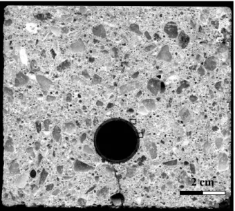
When looking under the microscope, thin secondary cracks and radial micro-cracks are detected, in accor-dance with the results of the simulations, as shown in fig-ures 7 and 8. Bright vertical lines on the steel surface can be observed that have been produced during the grinding process.
2 cm
Figure 6: General view of the crack pattern observed in a corroded sample
3.2 Resin impreganation
In order to improve the detection of the cracks, the slices were impregnated with resin and fluorescein under vac-uum. A low viscosity resin was selected to facilitate its penetration. The concentration of fluorescein was ad-justed by selecting among a set of five concentrations the smaller concentration that delivered good visibility of the mix under ultra violet (UV) light; a concentration of1,5 mg of fluorescein per millilitre of resin was finally used.
1 mm
Figure 7: Secondary cracks observed in a corroded sam-ple when looking under the microscope
1 mm
Figure 8: Radial micro-cracks observed in a corroded sample when looking under the microscope
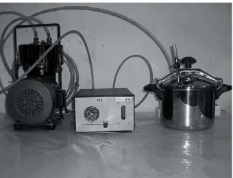
The slices were impregnated under vacuum to improve the resin penetration through the cracks and pores of con-crete. For that, a vacuum pump and a pressure cooker were utilised. A vacuum of 600 mmHg was reached. Firstly, vacuum was applied to the slice of concrete to empty of air the pores. Then, the resin was injected while keeping the vacuum. And finally the valve that controls vacuum was opened allowing the air to get inside. After curing the resin during two days at room temperature, the surfaces of the resin were ground again to eliminate the excess of resin and to expose undisturbed material.
In figure 10 a picture of the same slice that was stud-ied in figures 6-8 is shown after impregnation and under UV lighting. The secondary cracks and some microc-racks that were only observable under microscope before applying the surface treatment are now easily seen, and the overall pattern strikingly resembles the pattern in fig-ure 4.
impregna-tion, does not seem to have taken much resin during im-pregnation. The reason seems to be that the crack is full of compact black iron oxide. This seems to be true also for the root (next to the steel) of some secondary cracks.
Figure 9: Vacuum impregnation assembly. Pump, control of the pump and pressure cooker
2 cm
Figure 10: General view of the crack pattern obtained in a corroded sample after impregnating the surface with resin and fluorescein and lighting it with UV light
4 CONCLUSIONS
An interface finite element calledexpansive joint element
was programmed to simulate the expansion of the oxide layer that is generated when the rebars in reinforced con-crete structures are corroded and to study the mechanical effects of it over the surrounding concrete. The simula-tions with that model predict a wide main crack across the concrete cover but also six or seven long secondary
cracks and other smaller cracks, all of them much less opened than the main crack.
Very similar results are obtained when acceleratedly cor-roding real samples. Although only the main crack is clearly visible by the naked eye, secondary cracks and microcracks can be seen under the microscope, although in this way the wide-field view is lost, unless a wide mi-crograph covering is built.
The wide-field crack detection can be achieved by vaccuum-impregnating the samples with low viscosity resin containing fluorescein and observing them under UV light. The overall pattern of the fluorescent cracks closely resembles the patterns obtained numerically. The main crack and the root of some of the secondary cracks seems to be filled up with compact oxide.
ACKNOWLEDGEMENTS
The authors gratefully acknowledge the Ministerio de
Ciencia e Innovaci´on, Spain,for providing financial
sup-port for this work under grant BIA2005-09250-C03-01, and for providing, within the Spanish National Research Program CONSOLIDER-INGENIO 2010, funds for the research framework SEDUREC, within which the au-thors carried out their work. The auau-thors also thank Mr. Jos´e Miguel Mart´ınez for his help and advice during the setup of the experiments.
REFERENCES
[1] C. Andrade, M.C. Alonso, and F.J. Molina. Cover cracking as a function of bar corrosion: Part i - ex-perimental test. Materials and Structures, 26:453– 464, 1993.
[2] F.J. Molina, M.C. Alonso, and C. Andrade. Cover cracking as a function of bar corrosion: Part ii - nu-merical model. Materials and Structures, 26:532– 548, 1993.
[3] M.C. Alonso, C. Andrade, J. Rodriguez, and J.M. Diez. Factors controlling cracking of concrete af-fected by reinforcement corrosion. Materials and
Structures, 31:435–441, 1997.
[4] B. Sanz, J. Planas, A. M. Fathy, and J. M. Sancho. Modelizaci´on con elementos finitos de la fisuraci´on en el hormig´on causada por la corrosi´on de las armaduras. Anales de Mec´anica de la Fractura, 25:623–628, 2008.
[6] A. Hillerborg, M. Mod´eer, and P.E. Petersson. Anal-ysis of crack formation and crack growth in con-crete by means of fracture mechanics and fracture elements. Cement and concrete research, 6:773– 782, 1976.
[7] C. Geuzaine and J.-F. Remacle. Gmsh: a three-dimensional finite element mesh generator with built-in pre- and post-processing facilities. Interna-tional Journal for Numerical Methods in Engineer-ing, 79(11):1309–1331, 2009.
[8] G. V. Guinea, J. Planas, and M. Elices. A general bilinear fitting for the softening curve of concrete.
Materials and Structures, 27:99–105, 1994.
[9] M. Elices, G. V. Guinea, and J. Planas. On the mea-surement of concrete fracture energy using three point bend tests. Materials and Structures, 30:375– 376, 1997.
[10] J. Planas, G. V. Guinea, and M. Elices. Size effect and inverse analysis in concrete fracture.
Interna-tional Journal Fracture, 95:367–378, 1999.
[11] J. Planas, G. V. Guinea, J. C. Galvez, B. Sanz, and A. M. Fathy. Experimental determination of the stress-crack opening curve for concrete in tension. report 39. chapter 3. indirect tests for stress-crack opening curve. Technical report, RILEM TC 187-SOC Final Report, 2007.
APPENDIX: EQUATIONS OF THE EXPANSIVE JOINT ELEMENT
Theexpansive joint elementis defined by two parameters
as explained in the main text: the corrosion depthxand the volumetric expansion factorβ. The latter depends on the relation between the specific volumes of oxide and metal (per mole of metal):
β= vox vmet
−1 (1)
When external actions are applied simultaneously to the expansion of the oxide, the traction vectortcan be as-sumed (in the simplest model) to be linearly related to the apparent mechanical displacementwaand thus
writ-ten as
t=Knwa with wa=w−βxn, (2)
whereKnis the stiffness tensor,wis the total displace-ment,nis the unit normal vector to the metal surface, andwa is calculated as the difference between the total displacement and the free expansion displacement of the oxide. The stiffness tensorKnis a second order and ob-jective tensor that explicitly depends on the unit vectorn. It can be separated into the normal and tangent projec-tions to the surface as
Kn=knn⊗n+kt(1−n⊗n) (3)
where1is the second order identity tensor,⊗expresses tensorial product of two vectors andknandktare the
nor-mal and tangent stiffness constants. Substituting equation (3) in equation (2), the stresses vector is finally given by
t=kn(w·n−βx)n+kt[w−(w·n)n] (4)
Considering a pure shear stress τ that is applied to the oxide surface, the real displacementuat the application point is given by the sum of the shear displacement of the metal layer plus that of the oxide layer:
u=h−x τ Gmet
+ (1 +β)x τ Gox
(5)
wherehis the height of the layer of steel andGmetand
Gox are the shear stiffness moduli of metal and oxide.
The same displacement is calculated using the expansive joint element (which does not subtract thickness to the metal layer) as
u=h τ Gmet
+ τ kt
(6)
Mechanical equivalence between the expansive joint el-ement and the real metal-oxide system is established by identifying the displacements given by equations (5) and (6), so that the expansive joint shear stiffness is given by
kt=
G∗ox
βx , withG ∗
ox=
βGox
1 +β
1− Gox
(1 +β)Gmet −1
(7) whereG∗oxis the equivalent transversal stiffness modu-lus of the expansive joint element. Imposing mechanical equivalence when a normal stress is applied, similar re-sults are obtained for the normal stiffness:
kn=
Kox∗
βx , withK ∗
ox=
βKox
1 +β
1− Kox
(1 +β)Kmet −1
(8) whereKox∗ ,KoxandKmetare the normal stiffness
mod-uli of the expansive joint element, the oxide and the metal. It turns out, from the foregoing equation, that stiff-ness moduli of the element are inversely proportional to the corrosion depthx. To avoid numerical instability, a cut-off stiffness is established for a certain small valuex0
of corrosion depth and thus we write wherek0tandk0nare
the shear and normal stiffness corresponding tox0.
kt= (
kt0
kt0
x0
x
, kn = (
k0n ifx≤x0
k0n
x0
x ifx > x0
(9)
In the model, there is the possibility to distinguish two cases of normal stiffness for compression and tension. It is introduced by a directionality factorηso that
k0n=ηknc0 (10)
whereknc is the value of the stiffness for compression
andηis given by
η=
1 ifw·n−βx≤0(compression)
ηt ifw·n−βx >0(tension). (11)