HF spectrum activity prediction model based on HMM for cognitive
radio applications
L Melián-Gutiérrez
,
S. Zazo
,
J.L. Blanco-Murillo
,
I. Pérez-Álvarez
,
A. García-Rodríguez
B. Pérez-Díaz
A B S T R A C T
Although most of the research on Cognitive Radio is focused on communication bands above the HF upper limit (30 MHz), Cognitive Radio principles can also be applied to HF communications to make use of the extremely scarce spectrum more efficiently. In this work we consider legacy users as primary users since these users transmit without resorting to any smart procedure, and our stations using the HFDVL (HF Data+Voice Link) architecture as secondary users. Our goal is to enhance an efficient use of the HF band by detecting the presence of uncoordinated primary users and avoiding collisions with them while transmitting in different HF channels using our broad-band HF transceiver.
A model of the primary user activity dynamics in the HF band is developed in this work to make short-term predictions of the sojourn time of a primary user in the band and avoid collisions. It is based on Hidden Markov Models (HMM) which are a powerful tool for modelling stochastic random processes and are trained with real measurements of the 14 MHz band.
By using the proposed HMM based model, the prediction model achieves an average 10.3% prediction error rate with one minute-long channel knowledge but it can be reduced when this knowledge is extended: with the previous 8 min knowledge, an average 5.8% prediction error rate is achieved.
These results suggest that the resulting activity model for the HF band could actually be used to predict primary users activity and included in a future HF cognitive radio based station.
1. Introduction
Standard HF communications make use of the ALE (Automatic Link Establishment) protocol [1,2] which is frequently presented as an example of a primitive form
only transmit on their assigned channels that are expected to be available according to the experience of the radio operator.
Considering the previous issues, it is likely that as long as cognitive radio principles are introduced in HF stations, the radio frequency spectrum could be exploited in a more efficient way as HF stations will become aware of their surrounding environment and learn from it. In order to achieve such improvements in the band, these cognitive stations shall have the capability to change their operating parameters in order to adapt their transmissions to the available spectrum holes which are to be predicted by using the acquired knowledge.
In cognitive radio systems two types of users are distinguished: primary and secondary users. Primary users are those users that are holders of a license for a particular frequency band and therefore shall have prime access to it. Whereas, unlicensed users transmitting in that band are taken as secondary users as they are allowed to make use of it, but required not to interfere with communications coming from primary stations.
Due to the trans-horizon behaviour of HF communica-tions and the limited bandwidth where all HF users around the world can transmit, the difference between primary and secondary users relies on the smart and cognitive ca-pabilities of the HF user, so, in this work we will consider the primary ones to be the legacy users which transmit without resorting any smart procedure and consequently will interfere in our communications both on transmitter and receiver sides. On the other hand, our stations using the HFDVL (HF Data+Voice Link) architecture [3], which are also licensed for certain HF bands, hereafter will be considered as secondary users of the accessible frequency channels. Consequently, our stations must be able to pre-dict when the primary users start and finish their trans-missions, as they can interfere with transmitter and/or receiver sides, in order to send our own data packages by filling silence slots within primary transmissions. To do this, we shall use our broad-band HF transceiver [4] to se-lect those channels predicted as available. This architec-ture would be able to enhance the efficient use of the HF band and the performance of our HF communication sys-tem, provided that a suitable model for HF can be found.
A model of the primary user's dynamics in the band shall be extremely useful to make the best from the acquired knowledge in predicting the activity of the primary user in the channel. A predictive model is derived in this work for the HF band based on a set of Hidden Markov Models. It has been trained and validated on real data from the HF band as a first step towards a fully operative cognitive radio scheme for the band occupancy.
Attending to the modelling and detection problems, Hidden Markov Models (HMMs) are widely used for speech recognition [5] but more recently they have also been used on cognitive applications for primary user detection and prediction, where they have achieved remarkable results. A spectrum detection system based on several HMMs, each trained for a particular signal spectrum, was presented in [6]. Besides, channel state prediction models based on HMMs were proposed in [7,8]. The one addressed in [7] could only predict the channel state for
observation sequences of a 1 symbol period or 2 symbols period; and could not carry out the prediction of non periodic sequences as real measurements from a frequency band actually are. Furthermore, the model proposed in [8] was based on Higher-Order HMM and took into account the latency between spectrum sensing and Wi-Fi data transmissions. This model achieved a low average error rate with a prediction span of five time slots of 2 \xs each. As we will further discuss, this prediction span is smaller than the prediction span for our model in HF communications and the average error rates obtained cannot be compared to the ones presented here, as Wi-Fi data transmissions have also a smaller length than most common HF communications, which may last for several seconds.
Despite these previous contributions, most of the research in cognitive radio is related to communication bands above the HF band. Quite recently Koski and Furman introduced the challenges and opportunities of applying cognitive radio principles to HF communications in [9] and provided an overview of the concepts that could be considered for the next-generation ALE to introduce cognitive capabilities in [10]. However, to the best of our knowledge, no proposal for a real or simulated cognitive system for the HF band has been published yet.
Í.Í. Outline
The rest of the paper is organised as follows: the first part includes a description of the challenges of applying cognitive radio principles in HF communications in Section 2 and a brief introduction to Hidden Markov Models in Section 3.
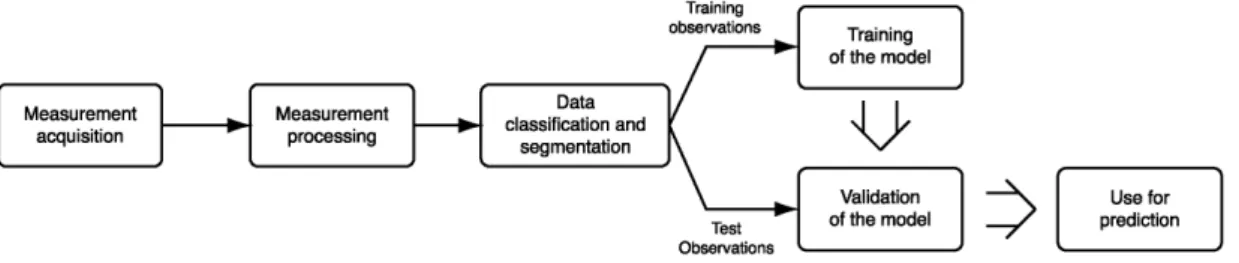
The second part describes the processes involved in the implementation of the HF primary user dynamics model detailed in the block diagram in Fig. 1. First, the acquisition of the measurements of the HF band is described in Section 4. Later, the measurement processing is depicted in Section 5, while observed sequences are then classified and segmented according to the criteria enunciated in Section 6.
The proposed HF primary user dynamics model is described in Section 7, where the training and validation processes are presented; whereas the prediction scheme developed and tested on top of this model is described in Section 8. Finally, conclusions on this work are drawn in Section 9.
2. Applying cognitive radio principles to HF communi-cations
Measurement acquisition
Measurement processing
Data classification and
segmentation
Training observations
Test
Training of the model
O
Validation of the model
: >
Use for prediction
Fig. 1. Block diagram for the training, testing and usage of the proposed HF primary user dynamics model in classification and prediction tasks.
characteristics which make this scenario different from the standard cellular one where cognitive radio concepts are usually being developed:
• Due to the traditional 3 kHz bandwidth for narrow-band voice use, the narrow-bandwidths available for HF communications are limited to 3 kHz.
• The limited extent of the HF band which is only 27 MHz wide, within which all HF communications around the world must be done.
• Due to these bandwidth limitations and the uncon-trolled trans-horizon transmissions, there are multiple collisions between legacy users as a result of the lack of coordination among them even if they use ALE protocol. • There are in-band and out-of-band interferences. These
out-of-band interferences affect the operation of any HF broad-band transceiver as in other bands, but the dynamic range of the received power is wider in the HF environment than in cellular environments. That is, transmitters inside a cell have a similar transmission power as they are relatively close to the receiver but in HF communications weak transmissions could be received from stations that are thousands of kilometres away and strong transmissions coming from stations that are very close to our receiver.
• As the two ends of a link are far away each other, the channel availability in each link direction is most likely to be completely different depending on the local interferences.
• The availability of one channel depends on two factors: if the point to point channel has appropriate propagation characteristics and also if it is already being used by other link at the receiver-side. It is important to remark that in HF links, which are half-duplex links, the receiver has to feedback the channel state information to the transmitter-side in order to notify if the sounded channel is available to transmit or not.
These HF characteristics must be considered in the HF cognitive station as a whole where the prediction model proposed in this contribution will be included to predict the activity of HF primary users.
3. Hidden Markov models
HMMs are a powerful and robust tool for modelling stochastic random processes as they are able to model a large variety of processes achieving high accuracy with rel-atively low model complexity. They have been extensively used in a myriad of signal processing applications dur-ing the last 20 years, mainly for fittdur-ing experimental data
onto a parametric model which can be used for real-time pattern recognition, and to make short-term predictions based on the available prior knowledge [5].
A Hidden Markov Model is defined as a doubly embedded process with an underlying stochastic process that is not observable. This hidden process (state) can only be evaluated through another set of processes that produce sequences that actually can be observed [5]. An HMM for discrete symbol observations is defined by the the following elements:
• A: State transition probability distribution matrix A = {cijj} of size N2 where N is the number of states in the
model and
dy = P [qt+1 = Sj\qt = Si] , 1 < i,j < N. (1)
The set of individual states is S = {Si, S2,..., SN} and
the state at time t is denoted as qt.
• B: The observation symbol probability distribution for state i, B = {jbj(k)}, where
bi(k)=P[Ot = Vk\qt = Si],
1 < i < N; 1 < k < M, (2)
Ot is the observation at time t and M is the number of
distinct observation symbols per state. The observation symbols correspond to the physical output of the system being modelled and are denoted as V = {Vi, v2,...,vM}.
• TI: The initial state probability distribution n = {JTJ} where
Tti = P[qi =Si], l < i < N .
• 0: Observation sequence
0 = 0 i 02- - - 0r
(3)
(4)
where each observation 0t is one of the symbols from
V and T is the number of observations in an observed sequence.
Thus, a complete definition of an HMM involves: two model parameters (N and M), the specification of the observations symbols and the specification of A, B and iz. In practise the compact notation used for an HMM will be
X = (A, B, TI) (5)
states are most frequently limited. An example of these models is the left-right or Bakis HMIV1 which has the property that as time increases the state index either increases or stays the same. Such a model was introduced to fit signals which changed over time in a successive manner, and is characterised by its transition matrix which forbids non-causal transitions within the models, i.e. its state transition coefficients have the property
% = 0, j <i (6)
as no transitions are allowed to states whose indexes are lower than that of the current state. Another relevant characteristic of a left-right HMM is that the state sequence must begin in state 1 and end in state N, so the initial probability distribution has the following property
Additionally, from an implementation perspective, such simplification introduces both a hard restriction and a relevant simplification for the model to be derived, as the number of parameters in the transition matrix decreases dramatically by almost a factor of 2.
Three major tasks must be fulfilled for a Hidden Markov Model defined as (5) to be useful in practical applications [5]:
1. Evaluation: Given an observed data sequence and a set of models to be compared, the probability that the provided sequence was produced by each of them, P(0\Xk), is to be computed as the cumulative
product of the likelihood obtained by each evaluated sample. This is calculated through the sum of the so called, terminal forward variables, aT(i), defined
in the "forward-backward" algorithm [5]. From the perspective of the Neyman-Pearson lemma, this can be considered as a scoring problem, in which the resulting scores will be used to decide which of the models fits the observed sequence better (i.e. obtained the largest accumulated likelihood value).
2. Decoding: Given an observation sequence, we choose a state sequence that is optimal in some meaningful sense. By doing this, we try to uncover the hidden part of the model according to some criteria. The most widely used criteria is to find the best state sequence that maximises the probability P(Q_, 0\X) using the well-known Viterbi algorithm [11].
3. Learning: The parameters of a particular model are adapted in order to maximise its likelihood when a set of sequences which correspond to the class it models is observed. The learning task is also referred to as the training of the model in which we attempt to find the model parameters which best describe the observed sequence (the training sequence). An iterative procedure such as the Baum-Welch method [5] is used to locally maximise the likelihood of the model defined asP(0\X).
Sections 7 and 8 are devoted to describe how the three tasks were developed in order to train and test the model, and also, to use them for prediction using a trained model.
4. Measurement acquisition
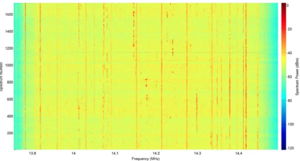
Real measurements from the HF band have been recorded to train and test the proposed model based on HMMs. The acquisition setup was located at IDeTIC facilities in Las Palmas de Gran Canaria and it is shown in Fig. 2. We have used our own broad-band transceiver [4] followed by a Vector Signal Analyzer (VSA) [12] and SystemVue Software [13], both from Agilent Technologies, to collect the time data from the Yagi antenna and convert it into frequency data (spectrum) by means of the Fast Fourier Transform (FFT) with the required characteristics. Several parameters, such as span, resolution bandwidth and number of bins for the FFT, must be adjusted while a suitable balance between them has to be observed to obtain the desired spectrum information. As it is shown in Fig. 2, our broad-band HF transceiver was required in the measurement system to collect data from the antenna which was then sent onto the Vector Signal Analyzer as the sensitivity of the VSA was not high enough and could not be used to reliably identify most of the HF signals in the band. Sequential measurements of the 14 MHz amateur band were carried out during three days in June and September 2011 with the acquisition setup shown in Fig. 2. These spectrum power measurements were collected in sample batches with a duration of 10 min, separated by intervals of 15 min. We have restricted our analysis to this band due to the limited bandwidth of our antennas, though the high-activity and the presence of all kinds of transmissions, both data and voice, observed within this band seemed to be a remarkable scenario to test and validate the proposed model.
Furthermore, depending on the day, the 14 MHz ama-teur band has different degrees of activity. There is normal activity on weekdays as can be observed in Fig. 3, while a huge amount of activity can be found at weekends, especially in those when amateur contests are scheduled, as can be observed in the collected data shown in Fig. 4.
The 14 MHz amateur band is in frequencies from 14,000 to 14,350 kHz and it is divided into three sub-bands:
• 14,000-14,065 kHz: CW signals.
• 14,065-14,100 kHz: Digital modulations such as PSK31 or 2-FSK.
• 14,100-14,350 kHz: SSB analog modulations.
In order to acquire spectral information from the whole band we have selected 14,175 kHz as the central frequency and a span of 500 kHz, though the collected span by VSA was actually wider than 500 kHz. With these parameters we obtained measurements of the amateur band and also channels outside of it that correspond to other radio sta-tions as it can be seen in the examples in Figs. 3 and 4. Given that all kinds of transmissions and activities take place in the acquired bandwidth, the 14 MHz band measurements are fairly representative of the main activities and trans-missions that can be found in the whole HF band.
Yagi
antenna Broad-band HF transceiver Vector Signal Analyzer Agilent
PC with: System Vue and
VSA software
Spectrum power ^measurement
Fig. 2. Measurement acquisition setup located at IDeTIC facilities in Las Palmas de Gran Canaria, Spain.
1200
I 300 a.
i
14.2 Frequency (MHz)
Fig. 3. Example of the acquired HF spectrum of the 14 MHz band with central frequency 14,175 kHz, span of 500 kHz and a duration of 10 min. Normal activity scenario.
1600
1400
1200
5 1000
1 1
1 300 (ft
600
400
200
!
1
••••
,•:
: :
"
1
1
1
60 |
14.2 Frequency (MHz)
Fig. 4. Example of the acquired HF spectrum of the 14 MHz band with central frequency 14,175 kHz, span of 500 kHz and a duration of 10 min. High activity scenario.
respectively, as detailed in Section 5. These sequences will be used as training and test sequences for the proposed model.
5. Measurement processing
The information captured by the VSA was processed to obtain the spectrum power of the whole acquisition band. Both frequency and time domain processing were applied to the collected data to obtain a time-frequency representation of the activity in each channel. Samples representing the mean power in a 3 kHz channel within a time slot of two seconds were obtained in this pre-processing step.
In the frequency domain, the collected spectrum is uniformly divided into channels of 3 kHz bandwidth as in the HF band; and the mean power is computed for each channel. Additionally, as the VSA computes the FFT of the wide-band measurement of 500 kHz span every two seconds approximately, the time resolution was defined in samples of approximately two seconds long. Finally, to complete the pre-processing step and obtain a reliable representation, time integration of the samples of the previous eight seconds of each channel is performed in order to best characterise the time evolution of the transmissions and avoid samples which represent the nulls of the HF channel and the typical impulsive noise present in this band.
Once channels are processed in time and frequency domains, the signal detection problem is set out to transform the power samples into normalised values. For this purpose, two hypotheses were defined:
H0 : x[n] = w[n] n = 1 , . . . , JV - 1
Hi : x[n] = w[n] + s[n] n = 1 , . . . , JV 1.
(8a) (8b)
H0 holds when there is only noise, w[n], in the channel
at sample n, while Hi is true when there is a signal, s[n], in the channel with additive noise at sample n. The detector that maximises the detection probability for a given false alarm probability is defined through the likelihood ratio test formulated in (9) as specified by the Neyman-Pearson lemma [14]
I(x) P ( x ; H i )
P (x; H0) > Y 0)
where p ( x ; H i ) is the probability distribution function for occupied-channel samples, p (x; H0) the probability
distribution for only-noise samples and the threshold y of the detector is derived from the false alarm constraint
Jv
p (x; H0) dx = a. (10)
The way to assess such a detector is to plot the Receiver Operating Characteristics (ROC) curve, which represents the detection probability (PD) versus the false
alarm probability (PFA) for different thresholds y. Given the
constrained false alarm probability a, the corresponding value of the threshold that maximises the detection probability can be found just by using the estimated ROC curve.
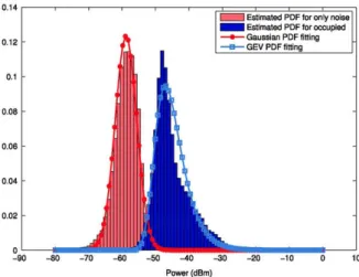
For these acquired measurements the probability dis-tributions for both hypotheses, p(x;H0) and p ( x ; H i ) ,
are estimated by computing the normalised histogram of the power of only-noise samples and occupied-channel samples, respectively. These estimations are plotted in Fig. 5 and as a result, threshold y can be defined. Further-more, in order to evaluate the ROC curve, the only-noise probability distribution has been fitted to a normal distribution N(/x0, cr0) with mean /x0 = —58.82, standard
deviation a0 = 3.23 and probability density function
P (x; H0)
1 (X-MO)
(11)
whereas the occupied-channel probability distribution has been fitted to a generalised extreme value distribution with location parameter \i = —47.125, scale parameter a = 3.882, shape parameter £ = —0.015 and probability density function
p ( x ; H i ) 1 1 + É x — [1
!±! _L+¡:><_±
(12)
As it can be observed in Fig. 5, the estimated probability distribution for hypothesis Hi can not be completely fitted to the proposed GEV distribution, but it is the best accurate fitting as it allows us to define the asymmetry of the estimated probability distribution from the acquired measurements. As opposed to the normal distribution, the GEV distribution can be used to fit data with non-zero skewness.
Once both distributions are fitted, the false alarm probability (PFA) and the detection probability (PD) are
computed to represent the analytic ROC plotted in Fig. 6 where
Jv
p (x; H0) dx
= l -e- (1 +^ ) ' (14)
and y is the detection threshold.
As it can be observed in Fig. 6, the analytic ROC could represent the mean behaviour of the acquired measurements as some experimental ROC curves are above the analytic ROC whereas others are below it.
6. Data classification and segmentation
Power (dBm)
Fig. 5. Estimation of the probability distribution of only noise-samples and occupied-channel samples and statistical fitting.
samples or occupied-channel samples, respectively. Subse-quently, these observation sequences are segmented into smaller sequences with a duration of one minute and clas-sified in order to reduce the variability of the trained sub-models (see Section 7).
As it can be observed in Figs. 3 and 4, different degrees of activity can be identified in the acquired channels. There are several channels which are almost unoccupied for long-time slots, while other channels remain occupied for the same amount of time and could not be used to transmit. Finally, there are other channels which could be used by a secondary user to transmit and make an efficient use of the band. So, we propose in this work a classification of the observation sequences prior to the stochastic modelling of the primary user's dynamics. This classification is based on the degrees of activity observed in the acquired measurements and the secondary user's behaviour in a cognitive radio system, that is:
• Available channels where the secondary user can transmit.
• Unavailable channels where a primary user is in the band and the secondary user cannot transmit.
• Partially available channels in which there are time intervals during which the secondary user can transmit until a primary user appears.
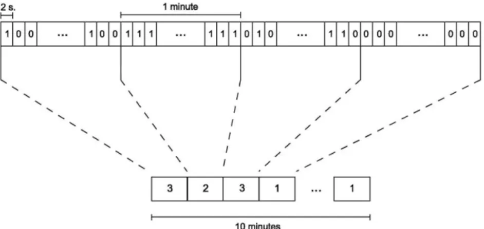
Observation sequences of ten and nine minutes long were segmented into one minute-long sequences as it can be seen in Fig. 7. These short sequences could be classified as 'Available', 'Unavailable' and 'Partially available' channels and encoded as {1, 2, 3}, respectively, to reduce the complexity of the model to be trained.
The criteria followed to classify the observation se-quences of each channel is based on the maximum time that a secondary user will need to transmit a data frame. Two thresholds were defined: one for minimum percent-age of occupation by a primary user in unavailable chan-nels, in such a way that the secondary user can transmit its maximum length data frame, and another for the max-imum percentage of occupation in available channels. In order to derive both thresholds, it is necessary to get the worst case of channel occupation as secondary users in
0 0.02 0.04 0.06 0.08 0.1 0.12 0.14 0.16 0.18 0.2
Fig. 6. Receiver Operating Characteristics (ROC).
HF data communications. This worst case scenario comes from assuming a maximum length for data frames to be transmitted by the secondary user. In this contribution, the frame of maximum length defined by the NATO Standard-isation Agreement STANAG 5066 [15] has been considered for our stations as secondary users. This standard estab-lishes the profile for professional HF data communications and defines frames, called D-PDU, that have 46 bytes of overhead and up to 1023 bytes of user data. Most HF data communications use a data rate of 600 bps or 1200 bps, and, with these parameters, the longest D-PDU frame re-sulting would last for 14.25 s (1069 bytes at 600 bps), which represents the worst case of channel occupation by the secondary user to be considered in our work.
2 s. 1 minute I—I I
Fig. 7. Data classification and segmentation.
7. HF primary user dynamics model
In this contribution Hidden Markov Models were used to model the primary users activity dynamics in the 14 MHz band. As it was described in Section 1, such a model could be used by our HFDVL stations, acting as secondary users, to predict the presence of a primary user, preventing interferences in their own transmissions. Therefore, this prediction would be the main source of information to avoid collisions with licensed users of the band, and consequently, to make the best possible use of the available frequency channels.
Once data from the HF band has been processed and classified, the activity model can be defined and trained. Due to the proposed classification of the observation se-quences, the model has a hierarchical structure and is de-fined as an ergodic HMM with three states interconnecting three underlying submodels, one for each class (i.e. avail-able, unavailable and partially available channel) as it can be seen in Fig. 8. These type of structures are commonly used in HMM based generative models as the one pre-sented in [16] for burst error characterisation.
Each submodel was trained with a set of one minute-long observation sequences from the corresponding class as previously defined (see Section 6) to derive a suitable model for the group at hand. Consequently, the first submodel was meant to characterise available channel sequences, the second submodel for unavailable channel sequences and the third one for partially available channel sequences. These submodels were implemented as left-right HMMs as the particular structure of the transition matrix they exhibit is quite suited to model the time evolution of the samples in the observation sequences, definitely better than ergodic models can, and with a reduced number of parameters to be trained.
In the end, the proposed model for primary user's dy-namics was built through the combination of a high-level, ergodic HMM with three states, each of them correspond-ing to available, unavailable or partially available chan-nels respectively, and a set of three left-right submodels. Each state in the upper model emits an observation se-quence of a minute long which is generated by the sub-model corresponding to that state. To simplify the training and evaluation of the high-level model, this was trained as
HMM., ) ( HMM2 ) [ HMM3
Fig. 8. High-level HMM of the interference model.
an independent HMM where each state only emits one sin-gle value representing the state, independently from the scores provided by the low-level submodels. That is, state Si only emits symbol '1' and it represents the observa-tion sequence generated by submodel 1. This also happens for states S2 and S3 emitting symbols '2' and '3',
respec-tively. So, the observation matrix for the high-level ergodic model, B, would actually be the identity matrix. Under this specification, observation symbols generated by the high-level model would be also the transitions between its states, that is, the transitions between the underlying sub-models. When the whole model is evaluated, the symbols for each state {1, 2, 3} correspond to the observation se-quences generated by the respective submodels for each of these states {1 (Available channels), 2 (Unavailable chan-nels), 3 (Partially available channels)} respectively and not these symbols.
Moreover, while submodels were trained to char-acterise one minute-long observation sequences from available, unavailable or partially available channels, the high-level model was trained to characterise the evolu-tion of a particular channel for ten and nine minute-long sequences, in which states are classified according to one minute-long sequences.
Once defined, the proposed model was trained and validated with the acquired data of Section 4.
7. Í. Training of the model
which maximises the probability that the observation sequences used for training were actually generated by the model. The Baum-Welch algorithm [5], based on the Expectation-Maximisation method, was used to train both submodels and the high-level model. Randomly initialised matrices were used for the first iteration of the Baum-Welch method, as no prior knowledge on the structure of the sequences was provided, and the amount of collected data seemed to be quite enough.
Due to the differences in the selected structures for the high-level model and the three sumbodels, two different training protocols were followed. Whereas the number of states of the high-level model was pre-fixed - 3 - due to the prior classification of the observations, the number of states for each submodel still had to be chosen. On the one hand, in training the proposed ergodic high-level model, our major concern was related to the initialisation of the values due to the ergodic structure itself. This structure had to be trained to be independent on the initial point, assuming that its execution could begin at any time, i.e. any of the three defined states could be the first. Thus, the transition matrix A, containing the estimated probability of going from one state to another regardless of the previous history, was initialised with different random seeds to reinforce the model stability, and trained on previously classified observation sequences including one minute-long available, unavailable and partially available segments.
On the other hand, the non-ergodic, left-right structure of the submodels largely reduced the complexity and cost for their training; unlike the high-level model for which no specific structure could be established. The number of states for the submodels, designed as left-right HMMs including three-states-long transitions (i.e. on each intermediate state, the incoming and outgoing transitions is equal and fixed to 4), was chosen according to the procedure previously described, based on the likelihood scores computed on every one minute-long observation sequences. For these submodels, matrices A and B were randomly initialised with a common seed, while TI was initialised as in (7) due to the left-right structure which forces the models to begin at the first state. Different configurations for these models including 20-45 states were trained with their own one minute-long observed sequences including binary samples containing information on channels' occupancy: the available channel submodel was trained with all sequences classified as available channels, and the same was done for unavailable and partially available channel submodels.
Once trained, submodels' accumulated likelihood sco-res were obtained according to the evaluation task de-scribed in Section 3, and the model with the maximum likelihood (highest P(0\X) among all trained models) was identified. However, a normalisation model built from the combination of all samples included was artificially in-troduced to normalise the likelihood scores and prevent spurious effects during their estimation. This slight modi-fication causes the former likelihood values to be bounded and behave as averaged likelihood ratios resulting from comparing different models to a common one, and there-fore allows positive and negative values. However, to com-pare the scores from two different models, the subtraction
,-io Available channel submodel
I •
20 25 30 35 40 45
Number of states
Unavailable channel submodel
20 25 30 35 40 45
Number of states
. „e Partially available channel submodel x 1 0
I ~205n A^^^^A^^A MS^A^A r^\,
20 25 30 35 40 45
Number of states
Fig. 9. Evolution of submodel log-likelihoods versus the number of states.
of these scores would still provide a relative cumulative log-likelihood ratio measure, independent from the inter-mediate artificial model introduced. Their assessment was carried out attending to the results depicted in Fig. 9. Fo-cusing on the curves included in this figure and corre-sponding to unavailable and partially available channel submodels, it should be noticed that the log-likelihood scores reach a local maximum for the configuration in which forty states were included, while log-likelihood scores corresponding to the available channel submodel were very small (see curve scale) for any number of states. Consequently, according to this result a suitable left-right HMM to model sequences included in the latter group could be built on any number of states from 20 to 45 with-out major differences. However, from a practical point of view we realised that if all submodels included the same number of states their comparison would be easier once the whole model was trained and used for prediction. Therefore, all submodels discussed hereafter are left-right Hidden Markov Models including forty states and up to three-states-long transitions as the one in Fig. 10.
Fig. 10. Left-right HMM with forty states and up to three states transitions.
7.2. Validating the proposed model
From the initial set of collected data, once the 70% have been put aside for the training of the HF primary user dynamics model, the remaining 30% were left to evaluate the trained model and validate it. As the HF primary user dynamics model was based on three submodels and a high-level model, the evaluation protocol required two steps: first, submodel likelihoods were evaluated with binary one minute-long sequences indicating the channel occupancy, and afterwards, the high-level model probabilities were calculated for each observation sequence of ten or nine minutes.
To compare all submodels, the evaluation problem must be solved taking the submodel with the highest likelihood as the local solution. A matrix containing values {1, 2, 3} was built from these decisions with its rows corresponding to the observation sequences of ten and nine minutes. Due to the definition of the high-level model in Section 7, these observation sequences were also equivalent to the transitions of the high-level model. Computing the difference between this generated matrix and the real one, we were able to estimate the percentage of wrong decisions, which reached the 5% of one minute-long test observation sequences.
As previously stated, the resulting matrix with {1, 2, 3} values contained the observation sequences for the high-level model and could be used to evaluate it. At this point it was not possible to compare models in order to solve the evaluation problem, but as these observation sequences were the same as the transition sequences due to the initial restriction on matrix B of the model, the decoding problem could be evaluated using the Viterbi algorithm [11]. The Viterbi algorithm was developed to identify the state sequence which maximises the probability P(Q_, 0\X), so that this state sequence can be directly compared to the observation matrix. The percentage of errors obtained was actually the same as the one obtained in the previous step, so, the high-level model can emit sequences such as the ones used in this test. Furthermore, if we think of it as a pseudo-random sequence generator, it would be able to emit random sequences statistically close to the real measurements used for its training, i.e. similar to the actual occupancy sequences found on the HF band.
8. Prediction scheme based on the HF primary user dynamics model
Bearing in mind the principles under cognitive radio and that the main goal of this model is to make an efficient use of the HF band, we propose its use to predict the activity of primary users in a particular HF channel. The following procedure was designed to predict whether a
channel will be used by a primary user within the next minute or not, and is based on the combination of the high-level model and the underlying submodels parametrised as HMMs, as described in the previous sections. Besides, due to the time variability of the HF channels and the absence of a low-delay feedback channel in HF half-duplex links, we have chosen a one minute prediction span, which is henceforth restricted for the designed prediction module.
The developed architecture shall operate according to the flow shown in Fig. 11. While a secondary user is sensing different channels in order to select the one that can be used to transmit without interfering with a primary user, it shall process the spectrum measurement corresponding to the last minute and use it as an observation sequence 0T to evaluate the three submodels
for available, unavailable and partially available channels. By evaluating the "forward-backward" algorithm, their likelihoods are computed and, instead of choosing the submodel with highest likelihood like in the evaluation process, the resulting probabilities can be used in the high-level model as updated entries for its observation matrix B.
Subsequently, the "forward-backward" algorithm is evaluated in the high-level model on the sequence of states corresponding to the prior T minutes and the three possible states for the next minute are evaluated: {1 (Available channels), 2 (Unavailable channels), 3 (Partially available channels)}. The state with the highest likelihood will be considered to be the predicted state for the channel in the next minute.
The average error rate of the prediction model with a prediction span of one minute is plotted in Fig. 12. Due to the time restriction on the data acquisition process which lasted for 10 min, most of the test sequences actually have a duration of nine minutes and thus, the maximum time span of the acquired knowledge is 8 min.
In addition to the global performance of the prediction model, performances for normal and high activity in the HF band are also presented in Fig. 12. As it was previously stated, the 14 MHz amateur band has a different behaviour depending on the day: there is a huge amount of activity at weekends, especially when amateur contests are scheduled, whereas there is a normal amount of activity on weekdays. Both situations have been considered in the training stage of the HF primary user dynamics model, so, the trained model will be able to predict whether a primary user will be present in the channel or not within the next minute in both situations.
Observations
£
oT?
t (min)
Submodel 1 X, = (A^B^n,)
Submodels
High-level model
^
PtOJA,)
1 f
B'n
Submodel 2 X2 = (A2,B2,n2)
V
P(0T|X2)
v
B'22
1 '
Submodel 3 A3 = (A3,B3,n3)
^
P(0T|X3)
^
B'33
B' =
B ' „ 0 0
0 B'22 0 0 0 B', '33
New definition of the high-level model:
i
High-level model X = (A,B',TT)
max(P(0T+1|X))
Predicted state
Previous
detected states T-2 T-1 t (min)
Fig. 11. Block diagram of the prediction procedure.
memory of the previous 8 min, the error rate is reduced to a 5.8%.
For high-activity environments, the average error rate of the prediction model increases to 16% when the secondary user has only listened the previous minute and it is reduced to 9.6% if the secondary user has a channel state memory of the previous 8 min. However, the average error rate decreases (respect to the global performance) to 8.7% in normal-activity environments with a channel state memory of the last minute and decreases to 4.7% when the secondary user has listened the previous 8 min.
8.1. Use of the HF spectrum activity prediction model
A comparative study of ALE-based stations with HFDVL stations using the proposed HF prediction model in terms
Acquired knowledge (min.)
Fig. 12. Average error rate of the prediction model.
the spectrum holes and transmit during these short time intervals not occupied by primary users.
In terms of link capacity, this fact will cause a higher capacity achievement with the HFDVL stations than the ALE-based stations when channels are partially available. The link capacity increase would then be related to the average percentage of time that the channel is actually available, provided that this is classified as a partially available channel. This situation takes place 69.73% of the time in our measurements. So, assuming that our HFDVL stations are transmitting an OFDM signal with 60 data subcarriers in a 3 kHz bandwidth HF channel [3], and that the noise power density is the same as the estimated for only-noise samples in Section 5, the capacity could be estimated as
<>;£(£".(••=?)) ™
where L is the number of measurements used for the computation, Nc is the number of OFDM subcarriers, Af
is the subcarrier spacing, H,-(k) is the channel frequency response at subcarrier k and measurement i and a^ is the noise power density, resulting in an estimated link capacity of 22,378 bits per second.
The capacity achievements of both stations will highly depend on the number of channels classified as par-tially available. If most of the sounded channels by both stations are available and only a few partially avail-able, there will not be a great difference between both stations. Nevertheless, if most of the sounded channels by both stations are classified as partially available, the HFDVL-based station with the HF prediction model will use the acquired knowledge to transmit in the spectrum holes without colliding with a primary user and, conse-quently, achieve a higher link capacity than the ALE-based station.
Merely as an example to illustrate this capacity increase, if we assume that channels are independent and there are 2 available channels, 1 occupied channels and 6 partially-available channels, the HFDVL station using the HF prediction model will achieve a global link capacity of
4 x C + 2 x (0.6973C) bits per second whereas the ALE-based station will achieve a lower global link capacity that will depend on the probability of collision if the ALE-based station decides to transmit in a partially available channel.
9. Conclusions
In this contribution we have proposed a primary user dynamics model for the HF band based on Hidden Markov Models. Due to the regulatory bandwidth restrictions and propagation characteristics of this frequency band, the use of this model to make predictions within the next minute of the activity in a particular channel is considered to be extremely helpful for cognitive stations acting as secondary users like our HFDVL based stations or any other standard HF modem using a 3 kHz HF channel.
The proposed model has been trained and validated with real measurements collected from the 14 MHz amateur band, and is built from three interconnected submodels which describe three types of channels: available channels, unavailable channels and partially available channels. Finally, we have used this model to predict the activity in a channel within the next minute and achieved an average 10.3% error rate when the acquired knowledge of the channel has a duration of one minute and reached an average 5.8% error rate when this knowledge is extended to the previous 8 min.
Furthermore, the use of this prediction model in our HFDVL-based stations would improve the efficient use of the band as it could be able to detect the spectrum holes and transmit when the predicted channel is classified as partially available. Due to the fact that the ALE-based station would not transmit due to the high collision probability with a primary user in a partially available channel, it has been shown that the HFDVL-based station could reach a higher channel capacity than an ALE-based station.
These results are very promising and show the possibili-ties of applying these prediction techniques in HF scenarios by means of cognitive radio principles.
Acknowledgments
This work has been mainly supported by the Spanish Ministry of Science and Innovation project TEC2010-21217-C02 and the Universidad de Las Palmas de Gran Canaria with a scholarship for postgraduate studies.
Projects TEC2009-14219-C03-01.TSI-020400-2011-35, FP7-ICT-2009-4-248894 WHERE-2 and the grant CONSOL-IDER-INGENIO 2010 CSD2008-00010 COMONSENS have also partially contributed.
References
[2] FED-STD-1045A Federal Standard, Telecommunications: HF Radio Automatic Link Establishment, General Services Administration, National Communications System Office of Technology & Standards, October 1993.
[3] I. Pérez-Álvarez, J. López-Pérez, S. Zazo-Bello, I. Raos, B. Pérez-Díaz, E. Jiménez-Yguacel, Real link of a high data rate OFDM modem: description and performance, in: 11th International Conference on Ionospheric Radio Systems and Techniques, IRST09, Edinburgh, UK, 2009.
[4] B. Pérez-Díaz, E. Jiménez-Yguacel, J. López-Pérez, I. Pérez-Álvarez, S. Zazo-Bello, E. Mendieta-Otero, Design and construction of a broadband (1 MHz) digital HF transceiver for multicarrier and multichannel modulations, in: 11th International Conference on Ionospheric Radio Systems and Techniques, IRST09, Edinburgh, UK, 2009.
[5] L. Rabiner, B.-H. Juang, Fundamentals of Speech Recognition, Prentice-Hall, 1993.
[6] Z. Chen, Z. Hu, R. Oiu, Quickest spectrum detection using hidden Markov model for cognitive radio, in: Proceedings of the IEEE Military Communications Conference, MILCOM, 2009.
[7] C.-H. Park, S.-W. Kim, S.-M. Lim, M.-S. Song, HMM based channel status predictor for cognitive radio, in: Proceedings of Asia-Pacific Microwave Conference 2007, 2007, pp. 1-4.
[8] Z. Chen, R. Qiu, Prediction of channel state for cognitive radio using higher-order hidden Markov model, in: Proceedings of the IEEE SoutheastCon 2010, 2010, pp. 276-282.
[9] E. Koski, W. Furman, Applying cognitive radio concepts to HF communications, in: 11th International Conference on Ionospheric Radio Systems and Techniques, IRST09, 2009.
[10] W. Furman, E. Koski, Next generation ALE concepts, in: 11th Inter-national Conference on Ionospheric Radio Systems and Techniques, IRST09, 2009.
[11] G. Forney, The Viterbi algorithm, Proceedings of the IEEE 61 (3) (1973)268-278.
[12] Agilent Technologies, VSA 89600, Technical Overview.
http://cp.literature.agilent.com/litweb/pdf/5989-1679EN.pdf, 2010. [13] Agilent Technologies, SystemVue documentation.
http://edocs.soco.agilent.com/display/sv201007/Home, 2010. [14] S.M. Kay, Fundamentals of Statistical Signal Processing: Detection
Theory, Vol. II, Prentice-Hall, 1998.
[15] STANAG 5066: Profile for HF Radio Communications, second ed., North Atlantic Treaty Organization (NATO), 2008.
[16] J. García-Frías, P.M. Crespo, Hidden Markov models for burst error characterization in indoor radio channels, IEEE Transactions on Vehicular Technology 46 (4) (1997) 1006-1020.
L. Melián-Gutiérrez received her M.Sc. in
Tele-communications Engineering in 2010 from the Universidad de Las Palmas de Gran Canaria (ULPGC) and her M.Sc. in Communication Sys-tems and Technologies in 2011 from the Uni-versidad Politécnica de Madrid (UPM). She is a Research Assistant at the Institute for Tech-nological Development and Innovation in Com-munications (IDeTIC), where she is working towards her Ph.D. in the fields of signal process-ing and Cognitive Radio with application to HF
A K
patterns.communications.
S. Zazo received his M.Sc. and Ph.D. in
Telecom-munications Engineering from the Universidad Politécnica deMadrid (UPM, Spain) in 1990 and 1995 respectively. From 1991 to 1994 he was with the Universidad de Valladolid and from 1995 to 1997 with the Universidad Alfonso X El Sabio (Madrid). In 1998 he joined UPM as I Associate Professor in Signal Theory and
Com-munications. His main research activities are in the field of Signal Processing with applications ' to Audio, Communications and Radar. More re-cently, he has been mostly focused on MIMO communications and Wire-less Sensor Networks from both physical layer and networking points of view.
J.L. Blanco-Murillo received his M.Sc. degree in
Telecommunications Engineering in 2007 and his M.Sc. degree in Communications, Systems and Techonologies in 2009, both from Univer-sidad Politécnica de Madrid (Spain). In 2007 he joined the Signal Processing Applications Group of this University, where he is currently pur-suing his Ph.D.. His research interests include statistical modelling and parameterization of complex systems, particularly for the character-ization and identification of abnormal speech
I. Pérez-Álvarez received his M.Sc. and Ph.D.
in Telecommunications Engineering from the Universidad Politécnica de Madrid (Spain) in 1990 and 2000 respectively. From 1989 to 1997 he worked for Europea de Comunicaciones SA. and Telefónica Sistemas S.A. He joined the Universidad de Las Palmas de Gran Canaria (Spain) as an Associate Professor in 1989. His main research activities are in the field of Signal Processing for Radio Communications.
A. García-Rodríguez is finishing his studies of
the M.Sc. in Telecommunications Engineering at the Universidad de Las Palmas de Gran Canaria. He is currently working as an Undergraduate Research Assistant at the Institute for Techno-logical Development and Innovation in Commu-nications (IDeTIC) and his M.Sc. thesis is related to the field of Signal Processing for Radio Com-munications.
B. Pérez-Díaz received his M.Sc. in