A control theoretic approach to solve a constrained uplink power dynamic game

A CONTROL THEORETIC APPROACH TO SOLVE A CONSTRAINED UPLINK POWER

DYNAMIC GAME

Santiago Zazo , Javier Zazo Matilde Sánchez-Fernández

ABSTRACT

This paper addresses an uplink power control dynamic game

where we assume that each user battery represents the system

state that changes with time following a discrete-time version

of a differential game. To overcome the complexity of the

analysis of a dynamic game approach we focus on the concept

of Dynamic Potential Games showing that the game can be

solved as an equivalent Multivariate Optimum Control

Prob-lem. The solution of this problem is quite interesting because

different users split the activity in time, avoiding higher

inter-ferences and providing a long term fairness.

1. INTRODUCTION

Dynamic Games and in particular Differential Games play a

very important role in Game Theory (GT) in many

applica-tions as economic and management science [1]. As already

stated, solutions are very complicated and just few simplistic

examples are known to have closed expressions while in most

of the cases, only approximate solutions by discretizing state

/ actions spaces or parameterizing value / utility functions are

affordable. On the other hand, there are just few publications

on Electrical Engineering [2]-[4] pointing out that researchers

start considering some dynamic effects on standard scenarios

that require more powerful tools to characterize the solutions

as number, uniqueness of Nash equilibria and also develop

algorithms for finding them. In this work we consider an

up-link scenario where a set of independent users need to define

individually the power that they are going to allocate at each

discrete time instant in order to maximize its achievable rate.

It should be noted that if a subset of users decide to transmit

at time t they are going to interfere to each other, thus

sig-nificantly decreasing the achievable rate of every user. Also,

each user has a limited battery for the transmission over time.

This scenario describes a dynamic game where users try to

transmit, the remaining battery represents the "state" of each

user, and the state together with the achievable rate define the

"utility" of each user. Finally the power that each user

de-cides to allocate at each time t is the "action". The discrete

time domain can be assumed in this scenario without loss of

generality since the users are not going to change their power

in a continuous way given that most communications system

define time intervals where the transmitted power need to be

fixed, for example time symbol or more generally frame

du-ration. In our case, this allows us to get closer relationships

between the problem formulation and the algorithmic

imple-mentation. Furthermore we consider an infinite (discounted)

horizon problem because our scenario is not constrained in

time, being the remaining energy of the battery the limitation

that will finish the game.

Our approach to solve the game is based on

reformulat-ing the game as an equivalent Multivariate Optimum Control

Problem (MOCP). This procedure, known as Dynamic

Po-tential Games [5], follows the same spirit as Static PoPo-tential

Games where the objective is to find an optimization control

problem whose solution coincides with the Nash equilibria of

the game. In many cases, it also provides information,

un-der certain hypothesis, about the uniqueness of the solution.

In dynamic scenarios, although the idea is similar, the

verifi-cation of the conditions needed by the game is not a simple

issue. The idea of Dynamic Potential Games has been very

recently formulated in [5] although the basic principles are

much older and originally developed by Dechert [6]-[9]. The

rest of the manuscript is organized as follows. Sec. 2

intro-duces the dynamic game framework and presents the game as

a MOCP. Sec. 3 formulates our uplink power game and

pro-vides the potential function to solve the game as a MOCP. Sec.

4, presents different approaches to solve the uplink power

MOCP and finally Sec. 5 and 6 show the simulation results

and the conclusions.

2. GAME AS A CONTROL THEORETIC PROBLEM

with xu G Xi and the set of actions of all players denoted in vector form as ut = {u\t... uit... v,Qt) where uit G W¿. The discrete time Dynamic Game can be represented by the following expression, where Vi:

V1 ( x o ) = m a x 2 , fí1^1 (XÍ J u t )

{_uít\ —~

s.t : Xf-i-i = / ( x t , U t ) , gi ( x t , Ut) < 0

(1)

Each user i intends to find the optimum sequence of actions {un} that maximizes its value function V1 (xo) expressed in terms of it own current and future (discounted) utility func-tion 7T* (xt, Uj). Parameter ¡3 < 1 is the discount factor. Very importantly, there is one constraint related to the time evolu-tion of the sequence of states { x t } typically depending on the previous state and current actions (Markovian model). Also, some extra constraints are included <?¿ (xí ? ut) < 0 because in most of the applications, states and actions are constrained. Solving these problems requires finding the sequence of ac-tions {u¿} that provide a Nash equilibria. Using similar con-cepts as in static games:

oo oo

E

where the equation must hold Vw¿t G W¿ and where u*t G W¿

represents the optimum action of user i at time t and u!_it

is the same concept for all users except i . We will see next that in practice, this optimization procedure is very compli-cated because each user has to solve a constrained optimum control problem where several coupled differential (or differ-ence) equations are involved. Typically, for open loop solu-tions, that is, u*t = •& (t) can be solved using the Maximum (or Pontryagin) Principle and for the closed loop (Feedback Markovian u*t = </> (x (t))) solving the Euler Equation. We should note that $ (t) and <f> (x (t)) are precisely the optimal actions’ trajectories to be determined.

We could solve the dynamic game in (1) by defining the Lagrangian for each agent and optimize. Then for the i-th player, including the corresponding multipliers we have:

L ( xt, ut,pt, \t) = ¿^t=o P 7r (.x*' u*/ +

-\-p\ ( / ( x t , Ut) — Xt-|-i) + \\gi ( x t , U t ) )

The first order condition for the optimization is given Vt:

iT—lt1 (Xf, Ut) + pliT— ( f ÍXí, Ut) — Xf+1 ) + A I TT—Q (Xt, Ut) = 0

(2)

(3)

and getting the dynamical equations by taking the Lagrangian derivatives with respect p\ and xi +i :

x t + i = / (XÍ J u t )

0~1pl = a 7rVx*+1 , U t+1 )

' f oxt+1 v ''T1'

Pi

(4)

t dxt-\-i 9i

including the complementary slackness condition and the positiveness of multiplier. It should be noted that the way to solve the game through the Lagrangian is by solving eqs. (3), (4) Vt and Vi.

An alternative to solve the game through eqs. (3), (4), is to follow a different approach defining our game as an equiv-alent Multivariate Optimum Control Problem.

We consider the following control problem for an as yet unspecified function I I (xi ? ut):

m a x á ' l l ( x t , ut) { u t } ^

s.t. : X t + i = / ( x t , U t ) , g ( xi ? ut) < 0

(5)

Similarly to what it is done in the game, we can find the

opti-mal solution from the Lagrangian:

(Xf, Ut,pt, Aj) = ¿^t=0 P ( H (.X*' U* / ~^~

+Pt ( / ( x t , Ut) — X t + i ) + Xtg ( x t , Uj)) (6)

by getting the partial derivatives in the Lagrangian variables. It should be noted that solving the optimization control prob-lem in (5) this way is a simpler probprob-lem than the optimization problem derived for the game in (3), (4) just by the fact that we drop the players dimensionality, however, its complexity may still be high enough to prevent obtaining the solution through the Lagrangian.

In order for the game in (1) to be equivalent to (5), func-tions 7T* must satisfy the following condifunc-tions Vi, j [6, 7]:

C1. 927T* 927 rJ

duidxj dxjdui

C2.a

C3.a

C3.b

927T* 927 rJ 927r* ,C2.b

927rJ

duiduj dujdui dxidxj dxjdxi

d dxj

d duj

d-K1

¿=i

Q

927T*

dui duidxA i=l J

/ ^ — d u i = /

^^ OUi ^^ dui

/ T;—d-Xi = / d , X i ^^i OXi *—? { dxiduj

If these conditions are fulfilled, the equivalent control

problem is finally given by:

11 ( x , u ) = > — a x i + > — d u i (7)

^^i OXi *—? OUi

3. UPLINK POWER DYNAMIC GAME AS A POTENTIAL DYNAMIC GAME

Let us now analyze the following particular game in the form of equation (1):

Algorithm 1 Multi-level Waterfilling Algorithm

1. Initialize uu for all» G Q and í e { 0 . . . N — 1}, k <— 0 and tolerance e.

2. For each ¿ e Q, do

(a) Compute S\ i + y ^ -^-1/Í--i i Uot , t G {0 . .. N — 1}

{w¿t}

i = 0

/3* log 1 + '¿í

1 i V ^ I 7 | 2

1 + ¿^ | rt-j Mjt

+ aíc¿í

(8)

S.£. .Xit-í-l Xfá Uit: xi0 -A-i

0 < v,it < [/jmax, 0 < Xjt < X4 m a x, Vi

m a x

m a x

assuming t as an integer variable. It can be noticed that the first term corresponds to maximizing a capacity term associ-ated to each user, where hi is the channel coefficient of user i and uit is the power used by user i at time t. The second term (parameter a is just a scaling parameter as a degree of freedom to weight properly both terms) corresponds to the state of that user defined as the battery level measured as the remaining power/energy left in the battery. Clearly, at every time step, the more power is used, the less remaining energy is left. Also, standard constraints on the instantaneous power and energy level apply. This problem is inspired on [10] but adding in this case one time-varying term representing energy consumption.

In Annex A we show that (8) fulfills the conditions to be solved as a MOCP where:

TT / \ ^ I 12 \ ^

11 (Xf, Ut) = l o g 1 + y , \hm\ umt + OL ?_,xit ( 9 )

(b) Set /XQ = maxj {£/™ax + S\} and /x* = 0

i. Calculate («o (&) = 0 2~0 and determine/x¿+1 (k)

for all t G {0 . . . N — 2}.

ii. Apply the waterfilling rule

r r m a x

uu (k) = [/x¿ (k) — Si] * t € {0 . . . N — 1}

iii. I f 2~^Í=O uit íí X™ax set 7*o *~ /4 (&), otherwise

¡il <— /x¿ (k).

iv. Set A; <— k + 1

v. Repeat from step (2(b)i) until /XQ — /x* < e

(c) Set «¿J <— uit(k) for player ¿

3. Repeat from step (2) until stopping criteria is met.

4.1. Waterfilling Algorithm

We propose first to solve the MOCP for a finite horizon for a sufficiently large time limit, allowing this way an efficient solution. Forming the Lagrangian from problem (10) with finite time horizon yields

Q Q

m=l ¿=1 £• (X*' U*' P*) = / ft 1°S ^ + / l^ml Wmi +

i = 0 m = l

Thus the equivalent control problem to the game in (8) is given by:

oo / / Q \ Q \

m a x \ ^ /? log 1 + \^ I ^m | umt + a N , xu

i = 0 m = l ¿ = 1 m a x

i ; s.i. : x ji +i = Xjt — «¿i, XJO = X^

o < W¿Í < u™

, o < x

< x™

yi

Q Q

+ a N Xjt + > p j (ÍC¿Í+I — ÍC¿Í + uu) ¿ = i ¿ = 1

s.i. 0 < «¿J < U™ax, pl>0, 0 < Xjt < X4 m a x, V¿, í

and solving for the control variables with the K K T condition dC/dun = 0 for all» G Q results into

(10)

uit I

i4

i + jy^i I ^ I 'if

i^¿r

MOCP given by (10), we can guarantee that its solution is a Nash equilibria of the original problem given by equation (8).

4. SOLVING THE GAME

Once it has been shown that we can solve the game as the control problem in (10), we will show next two approaches to solve the control problem avoiding the Lagrange approach explained in Sec. 2.

(11)

where [z]^ : = min {max {z, a} , 6}, t G { 0 . . . W — 1} and where p¿ represents the inverse of a water level to be deter-mined. To calculate these dual variables, the K K T condi-tion dC/dxit+i = —¡3t+1 ( a + p j+ 1) + ¡ilp\ = 0 of the

state variables provide the relation p!,-, = 4 p ! — a, t G {0 . . . N — 2} which form a recursive set of equations, for a given first value p}¡. The interpretation behind this result is graphically understood with water levels which are different from each other at all instants, but that are related with the adjacent slots as the steps of a staircase would be, where the max

position of every step is given by p\+i. This multi-level wa-terfilling is novel in its result, and can be formalized in Algo-rithm 1, where we have introduced water level variables ¡JL\ =

i for numerical reasons, that transform plt+1 into / 4+ 1 =

¡3¡JL\/\ — a.¡i¡i\. We have solved the MOCP by applying a Gauss-Seidel sequence of updates, where each control vari-able determines the interference parameters on step (2a) with the last known control variables from previously optimized players. In addition to this, we have used a bisection algo-rithm to determine the unknown water levels ¡JÍQ and recur-sively solved for t G {0 . . . N — 2}.

4.2. Iterative solutions based on Dynamic Programming

The control problem in (10) can be rewritten in a more com-pact way following Dynamic Programming Principles as:

V (xo) = m a x l l (xo, uo) + ¡ÍV ( / (xo, uo))

uo

s.t. : g (xt, ut) < 0

(12)

where I I (xi ? ut) follows the definition in (9) and g (xi ? ut) represent the boundary restrictions in (10). We can solve the previous problem iteratively by following a value function it-erative approach assuming that we are able to solve the right hand side of equation (12) obtaining Ug = h (xo) and substi-tuting back in (12) we get:

V (xo) = II (xo, h (xo)) + ¡iV ( / (xo, h (xo))) (13)

Given that V (•) is unknown in a first stage, we propose to iterate as shown in Algorithm 2. In practice, the loop ends when a certain condition on the stability of the solution is fulfilled. Policy iteration procedures can also be applied in a very similar way.

• * *

* * * * _*

" ' • • • • • • % • • •

!

\

1

s

1 *

. :

^

i

i

i * i *

*

i l

•

% %

%

• *

User 1 ^ ^ User 2 - - - User 3 • - • - User 4

60

40

20

10 20 30 40 50 60 70

Time

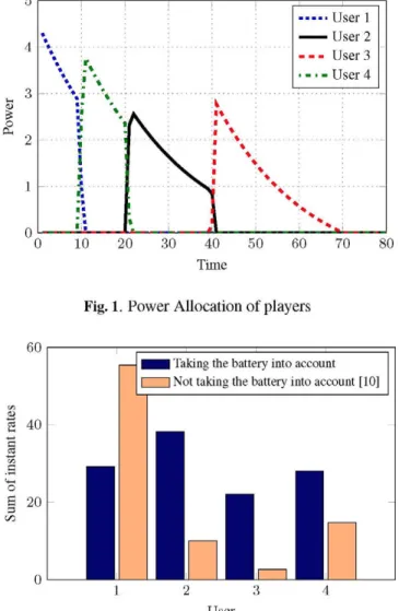
Fig. 1. Power Allocation of players

80

Taking the battery into account Not taking the battery into account [10]

1 2 3 4

User

Fig. 2. Comparison according to battery considerations

Algorithm 2 Value function iterative algorithm

1. Initialize VQ (X) = 0

2. for k = 0 to oo, do

(a) find hk (x) = argmaxu II (x, u) + ¡3Vk (g (x, u))

(b) Vfc+i (x) = II (x, hk (x)) + ¡3Vk (g (x, /ifc(x)))

5. RESULTS

In our simulation scenario we have considered Q = 4 players, a maximum transmit power level of U™ax = 5, total battery power X™ax = 33, forgetting value ¡3 = 0.95 and weight-ing value a = 0.001. We have simulated both alternatives given in previous section and they provide similar results, for that reason we just show here results for the waterfilling al-gorithm with time horizon N = 100. Channels are randomly obtained with zero mean gaussian complex distribution. We can observe in Figure 1 that players transmit in strict order where users that have better channels transmit first, and then

the rest. It seems, that this division in time avoids interfer-ence to other users, and allows to achieve the highest value in the potential function, and equivalently, in the game. This is the case, because the utility considers that running out of bat-tery is detrimental towards the device’s performance and so users decide to save battery until the channel becomes empty, coordinating to avoid collisions in time.

Finally in Figure2 we have plotted the total sum of instant capacities of each player as solved by Algorithm 1 (in blue) vs. the proposed algorithm in [10] that does not consider the state of the battery in its formulation (in orange):

'¿í argmax log 1 +

0 ≤ ui t≤ Um a x

i +

N

—"f\hi\ uu

with 7 = 0.1. With this comparison we simply state, that hav­ ing into consideration the battery life of the devices allows to transmit more information for the life duration of the network.

5

4

3

2

1

0 0

6. CONCLUSION

This work formulates an uplink power control scenario as a dynamic game, given that the battery of each user decreases as they assign power in different time slots. To further solve the dynamic game, first the game is reformulated as a con-trol problem, and latter waterfilling and iterative approaches are proposed to solve the control problem. The results show an interesting behavior where the users transmit in strict or-der following a channel quality criteria, that is the solution follows a scheduling philosophy.

A. A N N E X

We will prove next that TT'1 (xi ? ut) in (8) fullfils C1-C3 and then solve the line integral in (7) to get the potencial function

d27T¿ d2^

^ Q I 7 I 2 ^ /

The third equality results from the fact that i=\ I "¿I S is the derivative of the sum term in the denominator of the inte-gral. For the state term:

n ( x t , u t ) . C1 is trivial a a a a validate C2.a we proceed as follows:

= 0

dujdiij

1 |2 I |2 Ihi \hj v ^ 17 |2 1 + /Lm \h™\ "">*

yi,j. To

(14)

and due to the symmetric structure in (14), it is straight-forward to show that C2.a is satisfied. Identically for C2.b

TT-^Í— = TT-T,— = 0. And finally, for C3.a and C3.b we

OXiOXj OXjOXi

have:

Q

d-K1 Q 927T*

T;— / T;—dui = / 7 ; 7 : d u i = 0 ox-j *-^ dui ¿-^ OUiOXj

J i=l i=l J

O / ^ - ^ oír I s—^, O IT

— > — a x i = / T\7, dxi = 0 duj *-^ oxi ¿-^ oxiou-i

(15)

We solve now (7) in order to obtain the corresponding equiv-alent optimal control problem. Let us analyze each term in-dividually by defining £ : [0,1] —> (U\ x . . . x UQ) like a piecewise continuously differentiable path in the utility do-main with £i (0) = 0 and £¿ (1) = w¿ and r¡ : [0,1] —>• (X\ x . . . x XQ) like a piecewise continuously differentiable path in the state domain with rji (0) = 0 and rji (1) = x¿. We must recall that in this case, initial sate conditions would not be null because batteries start from a full level, but we have simplified the expression removing a constant term that is also considered when defining the constraints:

l Q

V~^ &~n v ^ / ^—dui = y

d-K1 (x, £) d£i(\)

¿ = 1 0 dui dX

dX =

£?=iN

dX =

o

o 1 + J2

\h

\ Cm (A) dX

/ \ ^ |7 | 2 ^ - | \ \ 1 / 1 , \ ^ 1 12 * (C\\ \

= log 1 + y , I"™. I Sm (J-J — i°g J- + /_, \hm\ U (U)

m m

f V~^ ^IT f V~^

/ T . d x i = y

^^ OXi 0 ¿-^

d-K1 (77, u ) dr/i (A)

dxi

1 Q

dx^ dX dX =

dr/i (A)

dX = a y r/i (1) — a y rji (0)

O •_-, dX z-^¡ ¿-^

Finally with the initial conditions defined before for £¿ (•) and rji (•) and introducing the time reference we get:

\

1 i \ ^ 17 i2 \ . \ ^ j- + y,I"™I Umt ~^~ay_j

m i=\

T T / \ ^ 17 12 \ ^

11 (Xf, ut) = log 1 + y , I"™. I Umt + a ?,xit

REFERENCES

[1] Engelbert Dockner, Differential Games in Economics

and Management Science, Cambridge University Press,

Nov. 2000.

[2] Tansu Alpcan, Tamer Baar, R. Srikant, and Eitan

Alt-man, “CDMA uplink power control as a noncooperative

game,” Wireless Networks, vol. 8, no. 6, pp. 659–670,

Nov. 2002.

[3] A. M. Mishra, “Bandwidth allocation with dynamic

se-lection in wireless networks,” in ICCCE 2012, April

2012.

[4] Kun Zhu, D. Niyato, Ping Wang, and Zhu Han,

“Dy-namic spectrum leasing and service selection in

spec-trum secondary market of cognitive radio networks,”

IEEE Trans. Wireless Commun., vol. 11, no. 3, pp.

1136–1145, 2012.

[5] Onesimo Hernandez-Lerma and David Gonzalez

Sanchez, Discrete Time Stochastic Control and

Dy-namic Potential Games: The Euler Equation Approach,

Springer International Publishing, Aug. 2013.

[6] Dee Dechert, “Optimal control problems from

second-order difference equations,” Journal of Economic

The-ory, vol. 19, no. 1, pp. 50–63, Oct. 1978.

[7] W. Davis Dechert, “Non cooperative dynamic games: a

control theoretic approach,” Unpublished. Available on

request to the author, 1997.

[8] W. D. Dechert and William A. Brock, “The lake game,”

Economic and Ecological Modelling, The Beijer

Insti-tute, The Royal Academy of Sciences, , no. 24, 2000.

[9] W. D. Dechert and S. I. O’Donnell, “The stochastic

lake game: A numerical solution,” Journal of Economic

Dynamics and Control, vol. 30, pp. 1569–1587, Sept.

2006.