DAY-TO-DAY VARIABILITY AND HABIT IN
MODAL CHOICES: A MIXED LOGIT MODEL
ON PANEL DATA
Elisabetta Cherchi, Dipartimento di Ingegneria del Territorio, Università di Cagliari,
Italy Mail: [email protected] and TRANSyT, Universidad Politecnica de Madrid.
E-Mail: [email protected]
Cinzia Cirillo Department of Civil and Environmental Engineering, University of
Maryland, College Park, MD 20742 USA Tel. +1 301 405 6864, Fax +1 301 405
2585, E-Mail: [email protected]
ABSTRACT
Understanding variability in individual behaviour is crucial for the comprehension of travel patterns and for the development and evaluation of planning policies. In the last 30 years a vast body of research has approached the issue in a variety of ways, but there are no studies on the intrinsic day-to-day variability in the individual preferences for mode choices and on the effect of habitual behaviours in absence of external changes. This requires using continuous panel data. Few papers have studied mode choice with continuous panel data but focused on the panel correlation. In this work we use a six-week travel diary survey to study the intrinsic day-to-day variability in the individual preferences for mode choices, the effect of habitual behaviour in the daily mode choices and the effect of long period plans. Mixed logit models are estimated that account for the above effects as well as for systematic and random heterogeneity over individual preferences and responses. We also account for correlation over several time periods.
Our results suggest that individual tastes for time and cost are fairly stable but there is a significant systematic and random heterogeneity around these mean values and in the preferences for the different alternatives. We found that there is a strong inertia effect in mode choice that increases with (or is reinforced by) the number of time the same tour is repeated. The sequence of mode choice made is influenced by the duration of the activity and the weekly structure of the activities. Finally, models improve significantly when panel correlation is accounted for. But it seems that inertia can explain to some extent for panel effect.
1. INTRODUCTION
Understanding variability in individual behaviour is crucial for the comprehension of travel patterns and for the development and evaluation of planning policies. As reported by Goodwin et al. (1990) variability is inherent in the travel choices because the system is not in equilibrium. In fact the environment changes incessantly and individual behaviours may at best be in continuous process of adjustment, searching for equilibrium but never reaching it. At the same time, even assuming that equilibrium is reached, environmental conditions might be different over days of the same week. As pointed out by Hirsh et al (1986) individuals select the current daily activity pattern based on the activity programs already realized and those planned for later periods. Hence, individual behaviour might be found varying simply because people's needs and desires vary over days of the same week. This later variability is often called day-to-day variability, or short-term or micro-dynamic effects (Clark et al., 1982). The variability due to adjustments to external changes (both changes in the transport supply and in the socio-economic characteristics) is often associated to long-term variability or macro-dynamic effects; because the adjustment cannot be instantaneous rather it usually takes time. It is important to mention that day-to-day variability can also be due to short-term adjustments, such as a change in the route or in the departure time. For example, one might choose a different time-of-day departure given the congestion experienced the day before. In this paper, we will refer to day-to-day variability as the ―planned‖ individual behaviour variability due to the daily/weekly activity pattern, opposite to the variation due to individuals adjusting their behaviours as a consequence of specific external changes, either in the long or short term.
In the last 30 years a vast body of research has approached the issue of the variability or (from the other side of the coin) the stability in individual behaviours in a variety of ways. Most of the researches have concentrated on the activity-based approach, where the analyses span from descriptive measures to more recent and complex dynamic models. Researches that have specifically studied the modal choices mainly used panel data collected at separate points in time (e.g. once a month or a year) to study the effect of inertia in mode choice after external changes. None have instead studied the intrinsic variability/stability in mode choice and the effect of habitual behaviours in absence of external changes. This requires using continuous panel data and the few papers that studied mode choice with this type of data focused on the panel correlation. Moreover, since individual choices are often based on daily or weekly activity programs, as mentioned before, it is likely that the current choice is affected not only by the choice made in the previous period but by all the choices made in the week or in a longer period.
The objective of this paper is to study the intrinsic day-to-day variability in the individual preferences for mode choices, the effect of habitual behaviour in the daily mode choices and the effect of long period plans (i.e. by means of the choices made during a period of several weeks). In particular, we aim at understanding whether the mode choice is affected by the whole plan of activities performed. Moreover, since the final goal of any modelling exercise is the policy assessment, we mainly focus on day-to-day variability of individual preferences over time and cost attributes, as these are crucial for the estimation of the subjective value of time.
performed by an individual, starting from a given base - home or workplace- end ending to the same base). Tours and sequences of tours allow the analysis of dependence among trips, the temporal organization (scheduling) of activities and the distinction between tours that involve one or multiple stops.
The remaining of this paper is organized as follows. Section 2 sets out the literature review on variability and habit in travel behaviour, and highlights the contribution of our analysis. Section 3 reviews the Mixed Logit models, briefly describes the dataset and defines the variables used in the final specification. Section 4 presents the modelling results. It is firstly reported an analysis of the systematic variability of the individual behaviours and then the results of the estimation of the mixed logit models with different correlation patterns are discussed. Concluding remarks and future research directions are summarized in Section 5.
2. LITERATURE REVIEW
The existence of time-varying components in transportation demand has been demonstrated in a number of studies, mainly developed in an activity-based context. For example, using a six weeks travel-activity diary (Mobidrive) collected in Germany by Axhausen et al. (2002), Bhat et al. (2005) examined the length between successive participations in several activity purposes. The Mobidrive data set has also been used by Yusak and Kitamura (2005) to examine the characteristics of action space and its day-to-day variation based on the representation of its extension by the second moment of activity locations it contains. Cirillo and Axhausen (2006a) proposed a discrete model for the choice of activity-type and timing; how past history (included by means of exogenous variables) affects activity choice and state dependence on different temporal dimensions is modelled via mixed logit. Copperman and Bhat (2007) examined time-use in children‘s activities, while Vanhulsel et al. (2007) introduced an extended reinforcement learning approach to produce weekly activity patterns in Belgium. Habib and Miller (2008) estimate a demand system model for daily activity program to study within-day and day-to-day dynamics in time-use.
A couple of papers, still adopting an activity-based framework, have explicitly analysed also the mode choices. Dargay (2005) estimated random effects ordered probit models to show that state dependence (last year‘s behaviour) is an important determinant of both car ownership and commute mode behaviour. Jara-Díaz et al. (2008) used the Mobidrive survey and a three-day activity record book collected in Santiago in 2003 to estimate a discrete-continuous model of mode choice and activity duration. Here only one representative trip is chosen for each week modelled in the activity model choice.
and perceived behavioural control. Dynamics in mode choice was also studied by Srinivasan and Bhargavi (2007) to account for rapid and substantial changes in fast growing Indian economy; data used for this model were recorded on two time points over a period of five years (2000–2005), although retrospective data collection was preferred over panel data. Finally, Yañez and Ortúzar (2009) and Yañez et al. (2010a) studied the effect of shock and inertia in individual behaviour using a five-day pseudo diary1 that has been repeated four
different times so far, just before and three times after the implementation of the radically new and much maligned Santiago public transport system (Transantiago) in Chile.
The day-to-day variability has received a good deal of attention in the past, but studies mainly aimed at analysing trip rates variations. Early works of Pas (1983, 1988) found that about 50 percent of the total variability in trip-making in the data set could be attributed to intrapersonal day-to-day variability in trip generation. In the same period, several interesting analyses on the variability and repetition of travel behaviour were conducted (see for example Pas and Koppelman, 1987; Kitamura and van der Hoorn, 1987; Jones and Clark, 1988; Hanson and Huff, 1988), but they focused exclusively on trip frequency. Anyway, it is important to highlight that these studies reached quite different conclusions in terms of day-to-day variability. As point out later by Huff and Hanson (1990) these results are ―hostage to the measures of travel used and to the length of time over which behaviour has been observed‖, this is why ―the picture of habitual behaviour that is emerging from these studies is blurred and fuzzy at best‖. In an attempt to find a middle ground of analysis Huff and Hanson (1990) investigated the recurrence of core stops and concluded that little of the day-to-day variability present in the individual‘s travel-activity pattern could be said to be regularly systematic. This result was later confirmed by Pas and Sundar (1995) who found considerable day-to-day variability in the trip frequency, trip chaining, and daily travel time in a three-day travel data survey.
More recently Bayarma et al. (2007) examined the recurrence structure of daily travel patterns using Markov chain models. Using the six-week Mobidrive survey their study revealed that some patterns tend to be pursued for a large number of consecutive days. Stopher et al. (2008) examined the effect of additional days of survey on measures such as the number of daily trips, the travel time per trip and per day, and the travel distance per day and per trip. They found that the variability in trip attributes exhibit no time dependent properties, but the need for multi-day data seems rather evident when looking at a longer period, for example a 15-day period, where the values obtained from a one-day survey are quite different from those obtained at the end of the period. Stopher et al. (2008) recognized that there is little information in the international literature on the effects of using multi-day data in modelling.
At best of our knowledge very few papers studied the day-to-day variability in the modal choice over a continuous period of time, but no one studied inertia effect in continous periods. Ramadurai and Srinivasan (2006) estimated a mixed logit model on mode choice to study within-day variability, but they do not actually study the day-to-day variability. In fact, their data only include two consecutive days, thus their approach is similar to the one used in short panel data, i.e. when information at few points in time are available. Moreover they focused on the variability in the choices, but do not study if individual preferences for tastes vary across days and weeks. Anyway, it is interesting to note that they found an inherent rigidity (inertia) among individuals to change modes. The inertial effect is particularly strong for bike and walk modes. They observe also transitional state-dependence between auto and
1 This is a unique survey where the diary was completed only for one day of the week, but
transit, as well as between walk and bike. Individuals who have chosen car in the previous tour have lesser propensity to choose mass transit or bike (compared to walk or ‗other‘ mode) as an alternative (to car) mode. Individuals who have chosen bike in the previous tour are more likely to select walk among the other modes in the current tour. They mention that this effect may be due to unobserved inherent preferences of individuals for non-motorized modes of travel, but such preference is not computed. Cirillo and Axhausen (2006b) instead estimated a mixed logit model on modal choice using a six-week travel survey (Mobidrive) but again they did not specifically study the day-to-day variability in modal choice. They focus on the random heterogeneity of the value of travel time savings. But inertia, systematic variation and correlation across random parameters are not accounted for. They concluded that heterogeneity exists around both the mean of time and cost, that positive values for time coefficients were possible for small fraction of the population and that VTTS varied across tour types and time of day. Cherchi and Cirillo (2008) studied the effect of repeated tours in a mode choice model using the Mobidrive survey, but they simply compared models estimated with and without repeated tours. Cherchi et al. (2009) again used the six-week panel data from the Mobidrive survey to estimate a mode choice model but they focused on ascertain the relative effects of correlation across individuals over two time periods: a single week and a day of the week -i.e. all Mondays- in the whole wave.
3. MIXED LOGIT MODEL ON MULTIDAY/WEEK DATA
The Mixed Logit (ML) is very suitable in case of panel data (Train, 2009). The ML utility function is characterised by an error term with at least two components: one that has the usual Extreme Value type 1 (EV1) distribution and allows obtaining the logit probability and the second () that accounts for the different components of unobserved heterogeneity, whose distribution can be chosen by the modeller. The ML probability is then the integral of standard logit probabilities, over a density of parameters f(
):( , ) ( )
qj qj
P
L b
f
d
(1)where Ω are the population parameters of the distribution2, b is a vector of fix parameters
and Lqj is the probability of individual q choosing alternative j conditional on the realization of . We are assuming here a typical parametric distribution, in which the shape of the distribution is specified a priori by the analyst.
When the ML is estimated using panel data, the correlation across observations provided by the same individual need to be accounted for. If j
j1,..., ,...,jt jT
is the sequence of choices made by each individual q, the probability (Pqj) of person q making this sequence of choices is the product of the conditional logit formulae, integrated over the density of the parameters:1,...,
( , ) (
)
t
q qj
t T
P
L b
f
d
j (2)
2 Namely the mean and standard deviation in distributions such as the Normal, Lognormal,and so on
The vector of unknown parameters is then estimated by maximizing the log-likelihood function, i.e. by solving the equation:
, , 1
max
,
max
Qln
q,
b
LL b
b
qP b
j
(3)This involves the computation of P bqj
,
for each individual q, which is impractical since it requires the evaluation of one multidimensional integral per individual. The value of P bqj
,
is therefore replaced by a Monte-Carlo estimate (SPqj) obtained by sampling over , and given by:
1
1
,
R
q qj
r
SP
L b
R
j (4)
where R is the number of random draws. As a result, b and are now computed as the solution of the simulated log-likelihood (SLL) problem:
( , ) , 1
1
max
,
max
Qln
q,
b
SLL b
bQ
qSP b
j
(5)We will denote by a
b,
R
*solution of this last approximation (often called Sample AverageApproximation, or SAA), while
b,
* denote the solution of the true problem (4).Equation (2) may have different degrees of complexity depending on the structure of the unobserved components. The vector of unobserved components can be decomposed to better capture the different aspects of individual random heterogeneity. As any other random utility model, the ML can also account for any type of systematic heterogeneity and non-linearity in the level-of-service attributes.
In this paper, we adopt a specification that accounts for systematic and random heterogeneity specific for each alternative and around the mean preferences for the level-of-service attributes. We tested as much individual variability as supported by the data and justified by the phenomenon. In particular we would like to avoid confoundign effects, i.e. that significant inertia and activities effects are actually due to unobserved inherent individual preference. The specification also allows for day-to-day variability and correlation among alternatives and over different time periods. The utility that person q obtains from alternative j
in each choice situation was specified as:
, , ,
,
t t t
qj x t x q x z q qj y y qj z q j qj
U b
b Z X b
b Z y
(6)where Xqjtis a vector of level of services variables, that vary among individuals q, alternatives j, and over time periods t; Zq is a vector of variables that vary among individuals but are fix
among alternatives and time periods. In our specification Zq includes four types of attributes:
socio-economic, locational, activity episode and inertia effects. x,q and y,qj are vectors of
individual parameters fixed over time periods but randomly distributed with mean zero and full variance-covariance matrix; bx,z and by are vectors of parameters assumed to be constant
period, it accounts for the day-to-day variability of the taste parameters3. Finally, y
j is a vector
of indices that equal one if the element appears in utility function of j, zero otherwise, allowing for error components and
t
qj
is the typical EV1 random term.It is important to mention that in this paper we account for correlation among repeated observations in panel data via (i) random parameters (RP) and (ii) error components (EC). The difference is that RP-panel generates correlation among all the alternatives, while the EC-panel generates correlation among a sub-set of (n-1) alternatives, and this might be confounded with NL forms. The RP-panel is usually preferred over the EC-panel method, but both methods have some advantages and some drawbacks. There is a discussion in the literature on which is the best way to account for panel effects but the problem is still open (see the discussion in Yañez et al., 2010b). Following Cherchi and Cirillo (2008) we also account for two dimensions of the correlation across responses (along each week and along the all panel), which are related with the dimension of the repeated variables tested in our specification.
3.1 Data set characteristics and variable specifications
The panel dataset used in this paper is derived from a six-week travel diary held in Karlsruhe (Germany) in 1999, part of the Mobidrive survey, which involved 160 households and 360 individuals in the main survey. Details on data collection techniques can be found in Axhausen et al. (2002) and in PTV AG et al. (2000)4. The recorded days were structured
according to activity chains on a daily basis and all trips were grouped into tours. A detailed description of the framework applied to the original Mobidrive survey to define the tours can be found in Cirillo and Axhausen (2006b). However, our sample slightly differs from the sample used in Cirillo and Axhausen (2006b). After conducting further tests on the availability of the alternatives, we also decided to concentrate only on the week days. Saturday and Sunday were excluded because, after a first round of modelling on a day-to-day basis, we found that, as expected, during the weekend individuals behave substantially different from the week days. The final sample is composed of 4089 single tours, 2488 daily schedules, 674 weekly schedules and 129 individual schedules, 56 household schedules.
The Mobidrive dataset is very rich. Other than the typical level-of-service variables (namely time and cost) it includes several socio-economic attributes related to both the individuals and their family, location variables, as well as all the activities performed. Before describing the variables calculated for our specification we would like to mention that in terms of mode chosen the sample is evenly distributed over the days of the week and over the six weeks. The characteristics of the tours are quite similar over the days and over the weeks, with few exceptions. The mode choice appears to be quite stable over days and weeks for all the modes, with few exceptions. But there not seems to be a clear pattern of variation over days. The same features occur when the analysis is repeated disaggregated for single purpose.
3 Our first specification also included a fix parameters specific for each time period to account for the
day-to-day variability in the ―pure‖ choice. However, given the high number of periods, we encountered problems in estimating such model.
4 See also http://www.ivt.ethz.ch/vpl/research/mobidrive for a list of the papers employing the
Socio-economic attributes
The socio-economic characteristics available in the dataset are the usual attributes measured in transport surveys: age, gender, number of children, professional status, education and so on. Some characteristics were included as single attributes (such as age and education), in other cases instead some profiles were defined (such as married with children and female working part-time). As described in the previous section, socio-economic characteristics were included as alternative specific attributes, to measure the difference in the preference for specific alternatives, and in interaction with the level of service attributes to account for systematic inter-personal variability variation in the preference for travel time.
Location attributes
The location attributes characterize the environment where people live. As well known there is a strong relation between mode choice and (sub-)urban characteristics. To measure this influence we then included a variable that indicates whether individuals live in an urban or sub-urban environment. Even in this case the effect of the location attribute was tested on both the preference for specific alternatives and the preference for travel time.
Inertia attributes
Inertia is advocated when the current choice is affected by the choice made in previous periods (state dependence) or by the value of some attributes in previous periods (lagged effect). In this paper we would like to take into account if individuals show inertia in the sequence of choices, but our panel data is characterised by uniform conditions (i.e. no changes occur in the supply conditions along the panel) and by a quite long (30 days) sequence of choice. In this sense, we could not strictly measure inertia as reported in Yañez
et al. (2010a,b) or in Ramadurai and Srinivasan (2006). We then decided to account for habit using lagged dependent variables. In particular the repeated tours (i.e. tours with the same characteristics, instead of only with the same mode) were used as a measure to account for habit. The following three variables were built:
1. A dummy variable which is equal to 1 if the tour characteristics (time, cost, purpose, mode, and so on) are equal to those of another tour already performed in a previous day (or previous moment of the same day).
2. A continuous weekly variable which counts the number of times the tour has been made in the previous days of the same week with the same characteristics (time, cost, purpose, mode, and so on). The variable then increases progressively with the days every time the same tour is repeated along the day of each week. But the count starts every new week.
3. A continuous six-week variable which counts the number of time the tour has been performed in previous days along the six weeks with the same characteristics (time, cost, purpose, mode, and so on). The variable then increases progressively with the days every time the same tour is repeated. The count is progressive over the six of weeks.
interpreted as the ―strength‖ of the habit. The second variable is calculated for each week separately, whereas the third for the entire period of the survey (i.e. six weeks).
Repeated tours may explain the preference for specific alternatives but also the major or less disutility for travel time. We also tested for the effect of the repeated tour specific for each activity. It is worth noting that other two variables (Miles Traveled and the Seasonal Tickets) are included in our model, these are also indicators of habit (Gärling and Axhausen, 2003).
Activities plan attributes
Mobidrive has a very rich description of the activities performed by each individual in each day of the 6-weeks survey. This gave us the very good opportunity to build some measures of the activity programs performed daily or during longer period and test whether and to which extent they affect mode choices. In particular, the following activity variables were calculated:
1. The Time Budget available (i.e. dedicated) to each activity in each day; 2. The total Time Budget available (i.e. dedicated) to each activity in each week;
3. The Number of Activity Episodes in each week, i.e. the cumulative number of times a given activity has been performed since Monday;
4. Whether an activity has been already performed during the same week (either with the same or different characteristics);
5. Whether an activity has been performed during the weekend;
6. Last time a given activity was done, measured as the number of days since the activity was performed last time;
7. Whether there was days were the individual did not make any trip.
All these variables were computed for each activity included in our analysis, which are: shopping, leisure, work, study, personal business, pick up/drop off and other activities.
4. MODEL RESULTS
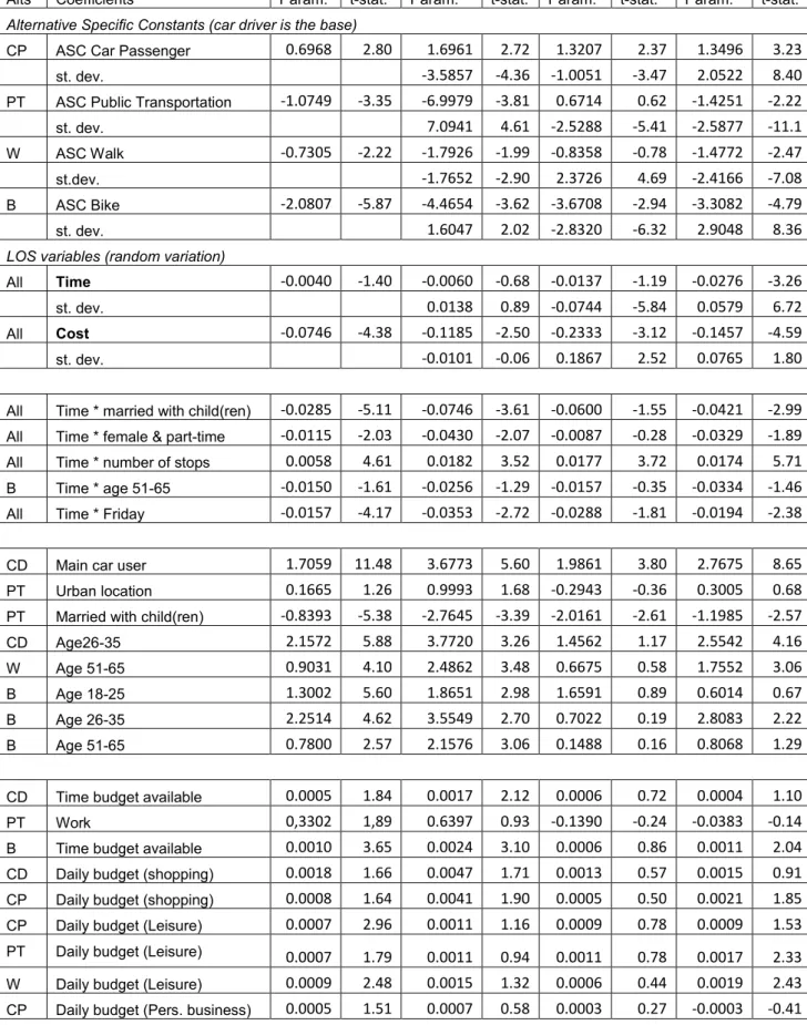
Using the dataset and the specification described in the previous section, several models were estimated accounting for, as much as possible, systematic taste variations, day-to-day variability, inertia and activity variables effect. Random heterogeneity in tastes for travel time and cost was also estimated and correlation among individuals over different time periods explicitly analysed. Table 1 reports the results of several ML models estimated with our best specification and different assumptions about correlation over observations. A simpler MNL allowing for systematic taste variations (parameterized effects) is also shown for comparison.
2 2
ˆ
ˆ
(
)
_
ˆ ˆ
ˆ
ˆ
2cov( ,
)
i j
i j i j
t test
(7)where
ˆ ˆ
i,
jare the mean parameters estimated for two different days or two different weeksand ˆ2, ˆ2
i j
their estimated variance. The t-test is asymptotically distributed Normal and gives the level of confidence we can reject the assumption of equality between pairs of parameters. We found that the parameters specific for each day and for each week were never significantly different from each other, with the only exception of the parameter corresponding to Friday. This result was found to be independent from the specification adopted. We started with a very simple specification including only time and cost and then we added all the other effects once at a time.Among the three ways of accounting for habit effects, the number of tours repeated along the six weeks provided the best results, especially in terms of log-likelihood. There seems to be a reinforcement effect of habit (captured by the continous variables) that is stronger over subsequent weeks than inside each single week. Models in Table 1 are then estimated specifying the inertia as a continuous six-week variable. As shown in Table 1, habit seems to have a positive effect for the non-motorized modes (walk and bike) but it reduces when the tour is made for leisure or personal business. This is in line with Ramadurai and Srinivasan (2006) who found that inertial effect is particularly strong for bike and walk modes. For car passengers instead there seems to be a tendency to change mode when repeating the same tours, as the repeated tours variables are always negative. Analogously the preference for public transport and walk decrease when the same tour is repeated for work or leisure. It is interesting to note that there is a preference for public transport when the tour is made for work. This is expected because work tours are usually systematic. However, the preference is not reinforced with the number of tours made (see the effect of the variable work and
repeated tour for work).
We found that the sequence of mode choice made over six weeks is not really influenced by the type of activity performed but rather by the duration of the activity and by the activities weekly structure. Firstly, it should be noted that, differently from the results on the habit effect, the activity variables were more significant when computed at weekly level, not during the six weeks. As expected we found that the time available (Time budget) is important only for the bike alternative, maybe because of the lifestyle associated with this type of mode. For all the other modes, what matters is the time dedicated to the activity during the day. The preference for a given mode is bigger when more time is dedicated daily (not in the specific tour) to the activity. The effect is different depending on the mode and on the activity. Having made shopping the same week decreases the utility of doing again shopping but only by public transport and walking; the same effect occurs for the purpose personal business. There is also an effect on the mode chosen due to the time passed since an activity was performed. The effect of shopping, leisure and pick-up/drop-off someone is strong, though it is not clear why this happens.
because activities are performed at each stop). Interestingly, some SE attributes lost significance with the inclusion of the variables accounting for activity and habit. In particular lost significance the location variables (living in suburban and using Public Transport) and the educational trips by Public Transport, Walk or Bike (students care less about travel time). Interactions with the cost attribute were also tested but none was found significant.
As for the preferences for each alternative, it is not surprising that Car Driver is preferred by people aged 18-35, and by those who are mainly car-users and travel many miles. At the same time, it is also not surprising that Public Transport is preferred only by seasonal ticket owners, whereas it is not liked for leisure trips, by older people or by those who have children. It is worth noting that variables such as miles travelled and possession of a season ticket are usual indicators of habit (Gärling and Axhausen, 2003).
Other than systematic variations, the data show also significant random variation in tastes and in preference among alternatives. Moreover, as we are using panel data an important issue is to account for correlation among observations. The Mixed Logit models reported in Table 1 differ for the way we account for correlation over observations. In the ML_ind the observations in the panel data were considered independent. Model ML_q (within-individual correlation) accounts for the full correlation across days and weeks reported by the same person. Model ML_w accounts for correlation across days of the same week (within-week correlation) but observations across weeks are independent. All models were estimated using a Normal distribution.
Regarding the effect of correlation over individuals in panel data, it can be noted that, as expected, models improve significantly when correlation is accounted for. Although, it is interesting to remark that the improvement is not always dramatic (see for example models
ML_ind and ML_w). It is also interesting to note that this result is due to the inclusion of the variable that explicitly accounts for the repetitions of the same tour. In fact, when models are estimated without the repeated tour variables, the effect of the correlation is much more marked (see results in Cherchi and Cirillo, 2007). At the same time it is important to note that the variables of the repeated tours seem to capture the effect of the correlation. Results in Table 1 show that when the repeated tours variable accounts for tours repeated along the six weeks (as in our models in Table 1) the correlation inside each week (Model ML_w) gives much better results than the correlation over individuals (i.e. over the six weeks, as in Model
ML_q).
Finally it is important to note that several variables loose significance depending on the type of correlation accounted for. This happens to some socio-economic variables (such as age) but mainly to the activities variables, especially to the time budget spent in other activities, shopping and leisure.
We also calculate the distributions of the value of travel time savings (see Figure 1). We note that the standard deviations of both time and cost coefficients in the mixed logit specification are not significant, perhaps because we are able to control large part of the systematic heterogeneity. When introducing correlation across weekly tours and individual tours, time and cost distributions are more disperse around the mean. The median VTTS for ML_ind is about 4.5 German Marks (GM) per hour, while values obtained with ML_w and the ML_q
specifications are higher and between 6.17 and 7.88 GM/hour. Large share of negative time values are also found when accounting for correlation.
0
0
j j
j j
P P P
P
(8)
where
P
j0 andP
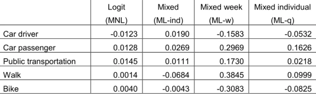
j are respectively the aggregate probabilities of choosing mode j before (do-nothing) and after introducing the measure, calculated by sample enumeration (Munizaga et al., 2000). Table 2 reports the market share variation computed by applying the different estimated models. It appears that logit and mixed logit produce similar results; the positive value for the cell corresponding to car driver probabilities deriving from Mixed Logit are due to numerical approximation associated to drawing from densities. Models accounting for correlation (ML_w and ML_q) produce more dramatic effects on modal shares and eventually different policy analysis results.5. CONCLUSIONS
In this paper we have used a six week travel diary from the German survey Mobidrive to study the intrinsic day-to-day variability in the individual preferences for mode choices, the effect of habitual behaviours in absence of external changes and the effect of long period plans (i.e. by means of the choices made during a period of several weeks). A mixed logit modal choices was estimated that allows accounting for interpersonal variability (systematic and random heterogeneity over individual preferences and responses) as well as correlation among individuals.
Since the final goal of any modelling exercise is the policy assessment, we mainly focus on day-to-day variability of individual preferences over time and cost attributes, as these are crucial for the estimation of the subjective value of time. We found that preferences for travel time and cost were stable over days and weeks, with the only exception of Friday, which shows a significant different travel time parameter. In particular travel time marginal disutility appears to be higher on Friday, maybe because this is the last day of the working week.
In this paper we also tested if individuals show inertia in the sequence of choices. Since our panel data was characterised by uniform conditions (i.e. no changes occur in the supply conditions along the panel) and by a quite long (30 days) sequence of choice, we used lagged dependent variables as a measure of individual habit. However, differently from previous studies, we measured how many times the tour has been repeated; which can be interpreted as the ―strength‖ of the habit. This inertia variable was calculated for each week separately, and for the entire period of the survey (i.e. six weeks). We also found that there is a strong inertia effect in the modal choice that increases with (or is reinforced by) the number of time the same tour is repeated. We also found that this effect is stronger over subsequent weeks than inside each single week.
We also found that the sequence of mode choice made over six weeks is not really influenced by the type of activity performed but rather by the duration of the activity and by the activities weekly structure. But, differently from the results on the habit effect, the activity variables were more significant when computed at weekly level, not during the six weeks. The preference for a given mode is bigger when more time is dedicated daily (not in the specific tour) to the activity. The effect is different depending on the mode and on the activity.
heterogeneity. We also found that models improve significantly when correlation is accounted for, which is consistent with findings from previous studies on panel data. However, an interesting result we found was that when inertia effect is properly accounted for, the inclusion of panel correlation produces a much smaller improvement in model fit. This is interesting because we have demonstrated that inertia can be measured and that rich behavioural explanation can be derived. On the other hand when panel correlation is basically a random variable we are just able to provide a measure of the ―error‖.
Table 1 - Model estimation results
Logit (MNL)
Mixed (ML_ind)
Mixed week (ML_w)
Mixed individual (ML_q)
Alts Coefficients Param. t-stat. Param. t-stat. Param. t-stat. Param. t-stat.
Alternative Specific Constants (car driver is the base)
CP ASC Car Passenger 0.6968 2.80 1.6961 2.72 1.3207 2.37 1.3496 3.23
st. dev. -3.5857 -4.36 -1.0051 -3.47 2.0522 8.40
PT ASC Public Transportation -1.0749 -3.35 -6.9979 -3.81 0.6714 0.62 -1.4251 -2.22
st. dev. 7.0941 4.61 -2.5288 -5.41 -2.5877 -11.1
W ASC Walk -0.7305 -2.22 -1.7926 -1.99 -0.8358 -0.78 -1.4772 -2.47
st.dev. -1.7652 -2.90 2.3726 4.69 -2.4166 -7.08
B ASC Bike -2.0807 -5.87 -4.4654 -3.62 -3.6708 -2.94 -3.3082 -4.79
st. dev. 1.6047 2.02 -2.8320 -6.32 2.9048 8.36
LOS variables (random variation)
All Time -0.0040 -1.40 -0.0060 -0.68 -0.0137 -1.19 -0.0276 -3.26
st. dev. 0.0138 0.89 -0.0744 -5.84 0.0579 6.72
All Cost -0.0746 -4.38 -0.1185 -2.50 -0.2333 -3.12 -0.1457 -4.59
st. dev. -0.0101 -0.06 0.1867 2.52 0.0765 1.80
All Time * married with child(ren) -0.0285 -5.11 -0.0746 -3.61 -0.0600 -1.55 -0.0421 -2.99 All Time * female & part-time -0.0115 -2.03 -0.0430 -2.07 -0.0087 -0.28 -0.0329 -1.89
All Time * number of stops 0.0058 4.61 0.0182 3.52 0.0177 3.72 0.0174 5.71
B Time * age 51-65 -0.0150 -1.61 -0.0256 -1.29 -0.0157 -0.35 -0.0334 -1.46
All Time * Friday -0.0157 -4.17 -0.0353 -2.72 -0.0288 -1.81 -0.0194 -2.38
CD Main car user 1.7059 11.48 3.6773 5.60 1.9861 3.80 2.7675 8.65
PT Urban location 0.1665 1.26 0.9993 1.68 -0.2943 -0.36 0.3005 0.68
PT Married with child(ren) -0.8393 -5.38 -2.7645 -3.39 -2.0161 -2.61 -1.1985 -2.57
CD Age26-35 2.1572 5.88 3.7720 3.26 1.4562 1.17 2.5542 4.16
W Age 51-65 0.9031 4.10 2.4862 3.48 0.6675 0.58 1.7552 3.06
B Age 18-25 1.3002 5.60 1.8651 2.98 1.6591 0.89 0.6014 0.67
B Age 26-35 2.2514 4.62 3.5549 2.70 0.7022 0.19 2.8083 2.22
B Age 51-65 0.7800 2.57 2.1576 3.06 0.1488 0.16 0.8068 1.29
CD Time budget available 0.0005 1.84 0.0017 2.12 0.0006 0.72 0.0004 1.10
PT Work 0,3302 1,89 0.6397 0.93 -0.1390 -0.24 -0.0383 -0.14
B Time budget available 0.0010 3.65 0.0024 3.10 0.0006 0.86 0.0011 2.04
CD Daily budget (shopping) 0.0018 1.66 0.0047 1.71 0.0013 0.57 0.0015 0.91
CP Daily budget (shopping) 0.0008 1.64 0.0041 1.90 0.0005 0.50 0.0021 1.85
CP Daily budget (Leisure) 0.0007 2.96 0.0011 1.16 0.0009 0.78 0.0009 1.53
PT Daily budget (Leisure) 0.0007 1.79 0.0011 0.94 0.0011 0.78 0.0017 2.33
W Daily budget (Leisure) 0.0009 2.48 0.0015 1.32 0.0006 0.44 0.0019 2.43
PT Daily budget (Pers. business) 0.0012 2.70 0.0022 2.36 0.0004 0.13 0.0009 1.01 Table 1 (continuous) - Model estimation results
Logit (MNL)
Mixed (ML-ind)
Mixed week (ML-q)
Mixed individual (ML-w)
Alts Coefficients Param. t-stat. Param. t-stat. Param. t-stat. Param. t-stat.
CD Daily budget (Other activities) 0.0013 2.72 0.0020 1.77 0.0002 0.01 0.0010 0.38
CP Daily budget (Other activities) 0.0024 6.36 0.0073 3.85 -0.0036 -0.39 0.0011 0.43 PT Daily budget (Other activities) -0.0049 -1.27 -0.0113 -1.01 0.0027 0.17 -0.0043 -0.50 W Daily budget (Other activities) -0.0027 -1.05 -0.0009 -0.13 0.0185 1.79 -0.0010 -0.17 CP Shopping in the same week -0.9030 -4.90 -3.3002 -3.32 -1.0824 -2.13 -1.3332 -4.31 PT Shopping in the same week -0.1901 -1.21 -0.2782 -0.95 -0.8011 -1.68 -0.4600 -1.25 CD Pick-up/drop-off same week -0.7956 -2.30 -1.8750 -1.97 -0.6381 -0.76 -0.9287 -1.83 CP Pick-up/drop-off same week -2.0435 -6.50 -7.4872 -3.76 -2.0299 -2.07 -2.0150 -3.80 PT Pick-up/drop-off same week -1.3786 -4.86 -2.2873 -3.00 -2.5734 -1.55 -1.5747 -2.39
CP Shopping in the weekend 0.5971 4.46 2.0322 2.95 0.2940 0.72 0.4184 1.28
CP Leisure in the weekend -0.3608 -2.92 -1.5826 -2.55 -0.1768 -0.57 -0.1788 -0.59
CD Last day of leisure 0.0419 2.87 0.1071 2.66 0.0388 0.59 0.0351 1.05
W Last day of leisure -0.0557 -4.33 -0.1156 -3.21 -0.0628 -1.08 -0.0799 -1.98
CP Last day of pick-up/drop-off 0.0265 5.98 0.0933 3.61 0.0115 0.84 0.0413 3.69
W Last day of pick-up/drop-off 0.0304 6.51 0.0551 3.66 -0.0017 -0.12 0.0273 1.98
CD Annual mileage 0.0163 2.16 0.0390 2.30 0.0302 1.27 0.0308 2.07
PT Number of Season Tickets 2.0651 13.98 9.4293 4.65 0.9194 1.26 2.7235 6.49
CP Repeated tour -0,5199 -5,56 -1.2646 -4.83 -0.5144 -2.69 -0.6950 -6.29
W Repeated tour 0,6235 5,24 1.5133 3.40 1.1652 4.48 1.2137 5.89
B Repeated tour 0,5621 4,69 1.3924 3.28 1.0803 4.56 1.1076 5.82
CD Repeated tours for leisure 0.9169 7.25 2.1529 4.64 0.9352 4.26 1.1870 5.49
CP Repeated tours for leisure -0.7613 -4.62 -2.7680 -3.31 -0.5793 -1.51 -0.9430 -3.38 W Repeated tours for leisure -0.2382 -2.76 -0.4310 -2.52 -0.4315 -2.74 -0.8249 -4.92 CP Repeated tours for p. business -0.5613 -2.70 -1.2030 -2.28 -0.7046 -1.55 -0.6880 -2.06 W Repeated tours for p. business -0.7228 -3.71 -1.4418 -2.78 -0.5427 -1.56 -0.9950 -3.37
PT Repeated tours for work -1.1569 -4.91 -2.1902 -3.14 -1.7810 -3.07 -1.8092 -3.85
W Repeated tours for work -0.2095 -2.16 -0.5032 -1.60 -0.2982 -1.59 -0.3476 -2.23
W Time * repeated tour -0.0096 -5.44 -0.0227 -3.50 -0.0188 -4.10 -0.0187 -4.79
B Time * repeated tour -0.0163 -5.03 -0.0401 -3.48 -0.0363 -4.72 -0.0346 -5.45
Figure 1: Inverse of the cumulative distribution function
Table 2 – Policy analysis: car cost increases by 30%
Logit (MNL)
Mixed (ML-ind)
Mixed week (ML-w)
Mixed individual (ML-q)
Car driver -0.0123 0.0190 -0.1583 -0.0532
Car passenger 0.0128 0.0269 0.2969 0.1626
Public transportation 0.0145 0.0111 0.1730 0.0218
Walk 0.0014 -0.0684 0.3845 0.0999
Bike 0.0040 -0.0043 -0.3083 -0.0825
REFERENCES
Axhausen, K.W., A. Zimmermann, S. Schönfelder, G. Rindsfüser and T. Haupt (2002). Observing the rhythms of daily life: A six-week travel diary. Transportation 29(2), 95-124.
Bayarma, A., Kitamura, R., and Y.O. Susilo (2007) On the recurrence of daily travel patterns: A stochastic-process approach to multi-day travel behavior. Transportation Research Record 2021, 55-63.
Bhat, C.R., S. Srinivasan, and K.W. Axhausen (2005), "An Analysis of Multiple Interepisode Durations Using a Unifying Multivariate Hazard Model," Transportation Research Part B, Vol. 39, No. 9, pp. 797-823.
Bradley, M. (1997) A practical comparison of modeling approaches for panel data. In T.F. Golob, R. Kitamura and L. Long (eds), Panels for Transportation Planning. Kluwer, Boston, 281-304.
Cherchi, E. y Cirillo, C. (2008) A modal mixed logit choice model on panel data: accounting for systematic and random heterogeneity in preferences and tastes. 86th Seminar on
Transportation Research Board. Washington DC, USA, (on CD).
Cherchi, E., Cirillo, C. and Ortúzar, J.de D. (2009) A mixed logit mode choice model on panel data: accounting for different correlation over time periods. International Conference on Discrete Choice Modelling. Leeds, UK, March, 2009. (on the website)
Cirillo, C. and Axhausen, K.W. (2006a) Dynamic model of activity-type choice and scheduling. Proceedings of the European Transport Conference, Strasbourg.
Cirillo, C. and K.W. Axhausen (2006b) Evidence on the distribution of values of travel time savings from a six-week travel diary. Transportation Research 40A, 444-457.
Clarke, M., Dix., M. and P Goodwin (1982) Some issues of dynamics in forecasting travel behaviour — a discussion paper. Transportation 11, 153-72.
Copperman, R., and C.R. Bhat. (2007) An Exploratory Analysis of Children‘s Daily Time-Use and Activity Patterns Using the Child Development Supplement (CDS) to the US Panel Study of Income Dynamics (PSID). Transportation Research Record 2021, 36-44.
Dargay J. (2005) The journey to work: an analysis of mode choice based on panel data. Paper presented at the European Transport Conference, Strasbourg, France.
Gärling, T. and Axhausen, K.W. (2003) Introduction: habitual travel choice. Transportation 30(1), 1-11.
Golob, T.F. (1990) Structural equation modelling of travel choice dynamics. In P.M. Jones (ed), Developments in Dynamic and Activity-Based Approaches to Travel Analysis. Aldershot, Hants, England, Gower, 343-370.
Goodwin, P.,R. Kitamura and Meurs, H (1990) Some Principles of Dynamic Analysis of Travel Demand. In P Jones (Ed.) Developments in Dynamic and Activity-Based Approaches to Travel, Gower/Avebury, Aldershot.
Hirsh, M., Prashker, J. and M. Ben-Akiva (1986) Dynamic model of weekly activity pattern. Transporation Science 20, 24-3
Habib, K.M.N. and E.J. Miller (2008) Modelling Daily Travel-Activity Program Generation Considering Within-Day and Day-to-Day Dynamics. Transportation 35, 487-848. Hanson, S. and J.O. Huff (1988). Systematic variability in repetitious travel. Transportation
15, 11-135.
Huff, J.O. and S. Hanson (1990) Measurement of habitual behavior: Examining systematic variability in repetitive travel. In: Jones, P. (ed) Developments in Dynamic and Activity-Based Approaches to Travel Analysis. Gower Publishing Co., Aldershot, England, pp. 229-249
Jara-Díaz, S.R. M.A. Munizaga, P. Greeven, R. Guerra and Kay Axhausen (2008) Estimating the value of leisure from a time allocation model. Transportation Research 42B (10), 946-957.
Jones, P. and M. Clarke (1988). The significance and measurement of variability in travel behaviour. Transportation 15, 65-87.
Munizaga, M. A., B. G. Heydecker, and J. de D. Ortúzar. (2000) Representation of Heteroscedasticity in Discrete Choice Models. Transportation Research Part B, Vol. 34, pp. 219–240.
Pas, E. (1983) A Flexible and Integrated Methodology for Analytical Classification of Daily Travel-Activity Behavior. Transportation Science 17(4), 405-429.
Pas, E. (1988) Weekly travel-activity behavior. Transportation 15, 89-109.
Pas, E. and Koppelman, F. (1987) An examination of the determinants of day-to-day variability in individuals' urban travel behavior. Transportation 14, pp. 3-20
Pas, E.I. and S. Sundar (1995) Intra-personal variability in daily urban travel behavior: Some additional evidence. Transportation 22, 135-150.
PTV AG, B. Fell, S. Schönfelder und K.W. Axhausen (2000) Mobidrive questionaires, Arbeitsberichte Verkehrs- und Raumplanung, 52, Institut für Verkehrsplanung, Transporttechnik, Strassen- und Eisenbahnbau, ETH Zürich.
Ramadurai, G. and K.K. Srinivasan, (2006) Dynamics and Variability in Within-Day Mode Choice Decisions: Role of State Dependence, Habit Persistence, and Unobserved Heterogeneity, Transportation Research Record 1977, 43-52.
Schlich, R. and Axhausen, K.W. (2003) Habitual travel behaviour: evidence from a six-week travel diary. Transportation 30, 113-36.
Simma, A. and K.W. Axhausen (2003). Commitments and modal usage – Analysis of German and Dutch panels, Transportation Research Record, 1854, 22-31.
Srinivasan, K. and P. Bhargavi (2007) Longer-term changes in mode choice decisions in Chennai: a comparison between cross-sectional and dynamic models. Transportation 34(3), 355-374.
Stopher P, E. Clifford and M Montes (2008) Variability of Travel over Multiple Days: Analysis of Three Panel Waves. Transportation Research Record 2054, 56-63.
Thøgersen, J. (2006) Understanding repetitive travel mode choices in a stable context: a panel study approach. Transport. Reserach A 40, 621–638.
Train, K. (2009) Discrete Choice Methods with Simulation. Cambridge, Inglaterra: Cambridge University Press.
Vanhulsel
,
M., Janssens, D. and Wets, G. (2007) Calibrating a new reinforcement learning mechanism for modelling dynamic activity-travel behaviour and key events. 86th Conference of the Transportation Research Board, Washington DC.Yáñez, M.F. and Ortúzar, J. de D. (2009) Modelling choice in a changing environment: assessing the shock effects of a new transport system. En S. Hess and A. Daly (Eds.), Choice Modelling: The State-of-the-Art and the State-of-Practice, Proceedings from the Inaugural International Choice Modelling Conference. Emerald, Bingley (forthcoming).
Yáñez, M.F., Cherchi, E., Ortúzar, J. de D. and Heydecker, B.G. (2010a) Inertia and shock effects over mode choice process: implications of the Transantiago implementation.
Transportation Science (under review).