Volume 2013, Article ID 528215,12pages http://dx.doi.org/10.1155/2013/528215
Research Article
Firefly Algorithm for Explicit B-Spline Curve
Fitting to Data Points
Akemi Gálvez
1and Andrés Iglesias
1,21Department of Applied Mathematics and Computational Sciences, E.T.S.I. Caminos, Canales y Puertos, University of Cantabria,
Avenida de los Castros s/n, 39005 Santander, Spain
2Department of Information Science, Faculty of Sciences, Toho University, 2-2-1 Miyama, Funabashi 274-8510, Japan
Correspondence should be addressed to Andr´es Iglesias; [email protected] Received 11 May 2013; Revised 8 September 2013; Accepted 13 September 2013 Academic Editor: Yang Xu
Copyright © 2013 A. G´alvez and A. Iglesias. This is an open access article distributed under the Creative Commons Attribution License, which permits unrestricted use, distribution, and reproduction in any medium, provided the original work is properly cited.
This paper introduces a new method to compute the approximating explicit B-spline curve to a given set of noisy data points. The proposed method computes all parameters of the B-spline fitting curve of a given order. This requires to solve a difficult continuous, multimodal, and multivariate nonlinear least-squares optimization problem. In our approach, this optimization problem is solved by applying the firefly algorithm, a powerful metaheuristic nature-inspired algorithm well suited for optimization. The method has been applied to three illustrative real-world engineering examples from different fields. Our experimental results show that the presented method performs very well, being able to fit the data points with a high degree of accuracy. Furthermore, our scheme outperforms some popular previous approaches in terms of different fitting error criteria.
1. Introduction
The problem of recovering the shape of a curve/surface, also known as curve/surface reconstruction, has received much attention in the last few years [1–14]. A classical approach in this field is to construct the curve as a cross-section of the surface of an object. This is a typical problem in many research and application areas such as medical science and biomedical engineering, in which a dense cloud of data points of the surface of a volumetric object (an internal organ, for instance) is acquired by means of noninvasive techniques such as computer tomography, magnetic resonance imaging, and ultrasound imaging. The primary goal in these cases is to obtain a sequence of cross-sections of the object in order to construct the surface passing through them, a process called
surface skinning.
Another different approach consists of reconstructing the curve directly from a given set of data points, as it is typically done in reverse engineering for computer-aided design and manufacturing (CAD/CAM), by using 3D laser
scanning, tactile scanning, or other digitizing devices [15,16]. Depending on the nature of these data points, two different approaches can be employed: interpolation and
approxima-tion. In the former, a parametric curve is constrained to
pass through all input data points. This approach is typically employed for sets of data points that are sufficiently accurate and smooth. On the contrary, approximation does not require the fitting curve to pass through the data points, but just close to them, according to prescribed distance criteria. Such a distance is usually measure along the normal vector to the curve at that point. The approximation approach is partic-ularly well suited when data are not exact but subjected to measurement errors. Because this is the typical case in many real-world industrial problems, in this paper we focus on the approximation scheme to a given set of noisy data points.
There two key components for a good approximation: a proper choice of the approximating function and a suitable parameter tuning. The usual models for curve approximation are the free-form curves, such as B´ezier, B-spline, and NURBS [17–26]. In particular, B-splines are the preferred
approximating functions because of their flexibility, their nice mathematical properties, and its ability to represent accurately a large variety of shapes [27–29]. The determi-nation of the best parameters of such a B-spline fitting curve is troublesome, because the choice of knot vectors has proved to be a strongly nonlinear continuous optimization problem. It is also multivariate, as it typically involves a large number of unknown variables for a large number of data points, a case that happens very often in real-world examples. It is also overdetermined, because we expect to obtain the approximating curve with many fewer parameters that the number of data points. Finally, the problem is known to be multimodal; that is, the least-squares objective function can exhibit many local optima [30,31], meaning that the problem might have several (global and/or local) good solutions.
1.1. Aims and Structure of This Paper. To summarize the
pre-vious paragraphs, our primary goal is to compute accurately all parameters of the approximating B-spline curve to a set of input data points. Unfortunately, we are confronted with a very difficult overdetermined, continuous, multimodal, and multivariate nonlinear optimization problem. In this paper, we introduce a new method to solve this fitting problem by using explicit free-form polynomial B-spline curves. Our method applies a powerful metaheuristic nature-inspired algorithm, called firefly algorithm, introduced recently by professor Xin-She Yang (Cambridge University) to solve opti-mization problems. The trademark of the firefly algorithm is its search mechanism, inspired by the social behavior of the swarms of fireflies and the phenomenon of bioluminescent communication. The paper shows that this approach can be effectively applied to obtain a very accurate explicit B-spline fitting curve to a given set of noisy data points, provided that an adequate representation of the problem and a proper selection of the control parameters are carried out. To check the performance of our approach, it has been applied to some illustrative examples of real-world engineering problems from different fields. Our results show that the method performs very well, being able to yield a very good fitting curve with a high degree of accuracy.
The structure of this paper is as follows: inSection 2 pre-vious work for computing the explicit B-spline fitting curve to a set of data points is briefly reported. Then, some basic concepts about B-spline curves and the optimization problem to be solved are given inSection 3.Section 4 describes the fundamentals of the firefly algorithm, the metaheuristic used in this paper. The proposed firefly method for data fitting with explicit B-spline curves is described in detail inSection 5. Then, some illustrative examples of its application to real-world engineering problems from different fields along with the analysis of the effect of the variation of firefly parameter 𝛼 on the method performance and some implementation details are reported in Section 6. A comparison of our approach with other alternative methods is analyzed in detail in Section 7. The paper closes with the main conclusions of this contribution and our plans for future work in the field.
2. Previous Work
Many previous approaches have addressed the problem of obtaining the fitting curve to a given set of data points with B-spline curves (the reader is kindly referred to [32–34] for a comprehensive review of such techniques). Unfortunately, many works focus on the problem of data parameterization and they usually skip the problem of computing the knots. But since in this work we consider explicit B-spline curves as approximating functions, our problem is just the opposite; the focus is not on data parameterization but on the knot vector. Two main approaches have been described to tackle this issue: fixed knots and free knots. In general, fixed-knot approaches proceed by setting the number of knots a priori and then com-puting their location according to some prescribed formula [6,9,18,19,22]. The simplest way to do it is to consider equally spaced knots, the so-called uniform knot vector. Very often, this approach is not appropriate as it may lead to singular systems of equations and does not reflect the real distribution of data. A more refined procedure consists of the de Boor
method and its variations [32], which obtain knot vectors so that every knot span contains at least one parametric value.
However, it has been shown since the 70s that the approximation of functions by splines improves dramatically if the knots are treated as free variables of the problem [30,31,35–38]. This is traditionally carried out by changing the number of knots through either knot insertion or knot removal. Usually, these methods require terms or parameters (such as tolerance errors, smoothing factors, cost functions, or initial guess of knot locations) whose determination is often based on subjective factors [31,39–43]. Therefore, they fail to automatically generate a good knot vector. Some methods yield unnecessary redundant knots [44]. Finally, other approaches are generally restricted to smooth data points [20,45–47] or closed curves [11].
In the last few years, the application of Artificial Intel-ligence techniques has allowed the researchers and prac-titioners to achieve remarkable results regarding this data fitting problem. Most of these methods rely on some kind of neural networks [1,8] and its generalization, the functional networks [3–5,7,21,23,48]. Other approaches are based on the application of metaheuristic techniques, which have been intensively applied to solve difficult optimization problems that cannot be tackled through traditional optimization algo-rithms. Recent schemes in this area involve particle swarm optimization [10, 13, 24], genetic algorithms [12, 49–51], artificial immune systems [25,52], estimation of distribution algorithms [11], and hybrid techniques [26]. As it will be discussed later on the approach introduced in this paper; also it belongs to this class of methods (see Sections4and5for more details).
3. Basic Concepts and Definitions
3.1. B-Spline Curves. Let U = {0 ≤ 𝑢0 = 𝑎, 𝑢1, 𝑢2, . . .,
𝑢𝑟−1, 𝑢𝑟 = 𝑏} be a nondecreasing sequence of real numbers on the interval[𝑎, 𝑏] called knots. U is called the knot vector. Without loss of generality, we can assume that[𝑎, 𝑏] = [0, 1].
The𝑖th B-spline basis function 𝑁𝑖,𝑘(𝑡) of order 𝑘 (or equiv-alently, degree 𝑘 − 1) can be defined by the Cox-de Boor recursive relations [38] as 𝑁𝑖,1(𝑡) = {1 if 𝑢𝑖≤ 𝑡 < 𝑢𝑖+1 0 otherwise (𝑖 = 0, . . . , 𝑟 − 1) , (1) 𝑁𝑖,𝑘(𝑡) = 𝑡 − 𝑢𝑖 𝑢𝑖+𝑘−1− 𝑢𝑖𝑁𝑖,𝑘−1(𝑡) + 𝑢𝑖+𝑘− 𝑡 𝑢𝑖+𝑘− 𝑢𝑖+1𝑁𝑖+1,𝑘−1(𝑡) (2)
for𝑖 = 0, . . . , 𝑟 − 𝑘 with 𝑘 > 1. Note that 𝑖th B-spline basis function of order 1 in (1) is a piecewise constant function with value 1 on the interval [𝑢𝑖, 𝑢𝑖+1) called the support of 𝑁𝑖,1(𝑡) and zero elsewhere. This support can be either an interval or reduced to a point, as knots 𝑢𝑖 and 𝑢𝑖+1 must not necessarily be different. The number of times a knot appears in the knot vector is called the multiplicity of the knot and has an important effect on the shape and properties of the associated basis functions (see, for instance, [29,32] for details). If necessary, the convention0/0 = 0 in (2) is applied. A polynomial B-spline curve of order𝑘 (or degree 𝑘 − 1) is a piecewise polynomial curve given by
𝐶 (𝑡) =∑𝑛
𝑖=0
𝑏𝑖𝑁𝑖,𝑘(𝑡) , (3)
where{𝑏𝑖}𝑖=0,...,𝑛are coefficients called control points as they roughly determine the shape of the curve and𝑁𝑖,𝑘(𝑡) are the basis functions defined above. For a proper definition of a B-spline curve in (3), the following relationship must hold:𝑟 = 𝑘 + 𝑛 (see [32] for further details).
In many practical applications, the first and last knots of U are repeated as many times as the order as follows: 𝑢0 = 𝑢1= ⋅ ⋅ ⋅ = 𝑢𝑘−1= 0, 𝑢𝑛+1= 𝑢𝑛+2= ⋅ ⋅ ⋅ = 𝑢𝑛+𝑘= 1 (such a knot vector is usually called a nonperiodic knot vector). In general, a B-spline curve does not interpolate any of its control points; interpolation only occurs for nonperiodic knot vectors. In such a case, the B-spline curve does interpolate the first and last control points [32]. Since they are the most common in computer design and manufacturing and many other fields, in this work we will restrict ourselves to nonperiodic knot vectors. Note however that our method does not preclude any other kind of knot vectors to be used instead.
3.2. The Optimization Problem. Similar to [49], let us assume that the data to be fitted are given as
𝑦𝑖= 𝐹 (𝑡𝑖) + 𝜖𝑖, (𝑖 = 1, . . . , 𝑁) , (4) where𝐹(𝑡) is the underlying (unknown) function of the data and𝜖𝑖 is the measurement error and we assume that𝑁 ≫ 𝑛. In this regard, a convenient model function, 𝑓(𝑡), for (4) is given by (3), where both the vectorB = (𝑏0, 𝑏1, . . . , 𝑏𝑛)𝑇 of coefficients and the vectorU of knots are considered as tuning parameters and(⋅)𝑇denotes the transpose of a vector or matrix. In the least-squares minimization of problem (4),
we determine the control points𝑏𝑗 (𝑗 = 0, . . . , 𝑛) of the B-spline curve𝑓(𝑡) by minimizing the least-squares error, 𝑄, defined as the sum of squares of the residuals as follows:
𝑄 =∑𝑁 𝑖=1 (𝑦𝑖− 𝑓 (𝑡𝑖))2=∑𝑁 𝑖=1 (𝑦𝑖−∑𝑛 𝑗=0 𝑁𝑗,𝑘(𝑡𝑖) 𝑏𝑗) 2 . (5)
Note that the objective function to be optimized,𝑄, depends on the B-spline coefficients and the interior knots. This problem is well known to be a continuous multimodal and multivariate nonlinear minimization problem [31]. In order to address this problem, in this paper we apply a firefly algorithm and obtain an accurate choice of bothU and B.
4. Firefly Algorithm
The firefly algorithm is a metaheuristic nature-inspired algo-rithm introduced in 2008 by Yang to solve optimization prob-lems [53,54]. The algorithm is based on the social flashing behavior of fireflies in nature. The key ingredients of the method are the variation of light intensity and formulation of attractiveness. In general, the attractiveness of an individual is assumed to be proportional to their brightness, which in turn is associated with the encoded objective function.
In the firefly algorithm, there are three particular ideal-ized rules, which are based on some of the major flashing characteristics of real fireflies [53]. They are as follows.
(1) All fireflies are unisex, so that one firefly will be attracted to other fireflies regardless of their sex. (2) The degree of attractiveness of a firefly is proportional
to its brightness, which decreases as the distance from the other firefly increases due to the fact that the air absorbs light. For any two flashing fireflies, the less brighter one will move towards the brighter one. If there is not a brighter or more attractive firefly than a particular one, it will then move randomly. (3) The brightness or light intensity of a firefly is
deter-mined by the value of the objective function of a given problem. For instance, for maximization problems, the light intensity can simply be proportional to the value of the objective function.
The distance between any two fireflies𝑖 and 𝑗, at positions
X𝑖 and X𝑗, respectively, can be defined as a Cartesian or Euclidean distance as follows:
𝑟𝑖𝑗= X𝑖− X𝑗 = √∑𝑑
𝑘=1
(𝑥𝑖,𝑘− 𝑥𝑗,𝑘)2, (6) where𝑥𝑖,𝑘is the𝑘th component of the spatial coordinate X𝑖 of the𝑖th firefly and 𝑑 is the number of dimensions.
In the firefly algorithm, as attractiveness function of a firefly 𝑗 one should select any monotonically decreasing function of the distance to the chosen firefly, for example, the exponential function as follows:
where 𝑟𝑖𝑗 is the distance defined in (6), 𝛽0 is the initial attractiveness at𝑟 = 0, and 𝛾 is an absorption coefficient at the source which controls the decrease of the light intensity.
The movement of a firefly𝑖 which is attracted by a more attractive (i.e., brighter) firefly𝑗 is governed by the following evolution equation:
X𝑖= X𝑖+ 𝛽0𝑒−𝛾𝑟𝑖𝑗𝜇(X
𝑗− X𝑖) + 𝛼 (𝜎 −12) , (8)
where the first term on the right-hand side is the current position of the firefly, the second term is used for considering the attractiveness of the firefly to light intensity seen by adjacent fireflies, and the third term is used for the random movement of a firefly in case there are not any brighter ones. The coefficient𝛼 is a randomization parameter determined by the problem of interest, while 𝜎 is a random number generator uniformly distributed in the space[0, 1].
5. The Proposed Method
In this section, the firefly algorithm described in previous paragraphs is applied to obtain the approximating explicit B-spline curve of a given set of noisy data points expressed according to (3)-(4). To this aim, in this work we consider four different fitness functions. The first objective function corresponds to the evaluation of the least-squares function, given by (5). Since this error function does not consider the number of data points, we also compute the RMSE (root-mean squared error) given by
RMSE= √∑
𝑁
𝑖=1(𝑦𝑖− ∑𝑛𝑗=0𝑏𝑗𝑁𝑗,𝑘(𝑡𝑖))2
𝑁 .
(9)
Note, however, that the best error might be obtained in either (5) or (9) at the expense of an unnecessarily large num-ber of variables. To overcome this limitation, we also compute two other fitness functions: Akaike Information Criterion (AIC) [55,56] and Bayesian Information Criterion (BIC) [57]. Both are penalized information-theoretical criteria aimed at finding the best approximating model to the true data through an adequate trade-off between fidelity and simplicity. They are comprised of two terms: the first one accounts for the fidelity of the model function, while the second one is a penalty term to minimize the number of free parameters of the model,𝜂. They are given, respectively, by
AIC= 𝑁log𝑒(𝑄) + 2𝜂,
BIC= 𝑁log𝑒(𝑄) + 𝜂log𝑒(𝑁) . (10) A simple comparison between (10) shows that both criteria are quite similar, but BIC applies a larger penalty than AIC. Thus, as other factors are equal, it tends to select simpler models than AIC (i.e., models with fewer parame-ters). Both methods provide very similar results for smooth underlying functions. Differences might arise, however, for functions exhibiting sharp features, discontinuities, or cusps. In particular, AIC tends to yield unnecessary redundant knots
and, therefore, BIC becomes more adequate for such models. A great advantage of AIC and BIC criteria is that they avoid the use of subjective parameters such as error bounds or smoothing factors. Furthermore, they provide a simple and straightforward procedure to determine the best model: the smaller their value, the better fitness. Because of that, we use them to select the best model for our examples and to compare our results to those of other alternative approaches. Before searching a solution to the problem, two sets of control parameters must be set up. The first set corresponds to the curve parameters: the number of control points and the order of the B-spline curve. In general, they are freely chosen by the user according to the complexity of the shape of the underlying function of data and the requirements of the particular problem under study, with the only constraint that𝑛 ≥ 𝑘. The second set of parameters relates to the firefly algorithm itself. As usual when working with nature-inspired metaheuristic techniques, the choice of control parameters is very important, as it strongly influences the performance of the method. Although some guidelines are given in the literature to tackle this issue, such a selection is problem-dependent and, therefore, it remains empirical to a large extent. In this paper, our parameter tuning is based on a combination of both theoretical results found in the literature of the field and a large collection of empirical results. From the former, it is well known that the value of absorption coefficient, 𝛾, is important in determining the speed of convergence and the behavior of the method. In theory,𝛾 ∈ [0, ∞), but in practice values in the extremes should be avoided. When𝛾 → 0 the attractiveness becomes constant, which is equivalent to say that the light intensity does not decrease with distance, so the fireflies are visible anywhere, while that 𝛾 → ∞ corresponds to the case where the attractiveness function in (7) becomes a Dirac𝛿-function. This case is equivalent to the situation where the fireflies move in a very foggy environment, where they cannot see the other fireflies and hence they move randomly. In other words, this corresponds to the case of a completely random search method. Based on this analysis, we carried out thousands of simulations to determine a suitable value for𝛾 and found that the value 𝛾 = 0.5 provides a quick convergence of the algorithm to the optimal solution. Regarding the initial attractiveness,𝛽0, some theoretical results suggest that𝛽0= 1 is a good choice for many optimization problems. We also take this value in this paper, with very good results, as it will be discussed in next section. For the potential coefficient,𝜇, any positive value can be used. But it is noticed that the light intensity varies according to the inverse square law, so we set up𝜇 = 2 accordingly. Finally, a stochastic component is necessary in the firefly method in order to allow new solutions appear and avoid to getting stuck in a local minimum. However, larger values introduces large perturbations on the evolution of the firefly and, therefore, delay convergence to the global optima. In this work, we carried out several simulations to determine the optimal value for this parameter 𝛼 and finally we set up its value of 0.5 for this randomization parameter. The reader is referred toSection 6.4for a more detailed discussion about how the variation of this parameter affects the behavior of our method.
Once the parameters have been set up, the firefly algo-rithm is executed for a given number of fireflies, representing potential solutions of the optimization problem. Each firefly in our method is a real-valued vector of length𝑛 − 𝑘 + 1, initialized with uniformly distributed random numbers on the parametric domain[0, 1] and then sorted in increasing order. In this work, an initial population, 𝑛𝑓, of fireflies is considered. Its value is set up to𝑛𝑓 = 100 in all examples of this paper. We also tried larger populations of fireflies (up to1000 individuals) but found that our results do not change significantly. Since larger populations mean larger computation times with no remarkable improvement at all, we found this value to be appropriate in our simulations.
This initial population is then subjected to the firefly mechanism and least-squares minimization, yielding a col-lection of new solutions to the optimization problem (5). In our executions we compute independently all four fitness functions indicated above, meaning that our simulations are to be repeated for each fitness function. On the other hand, each simulation is repeated several times according to a parameter𝜅 in order to remove the spurious effects of randomization typically arising in any stochastic process. In this paper, we consider a value of𝜅 = 20, meaning that each simulation is independently carried out 80 times to obtain the final results. Each execution is performed for a given number of iterations,𝑛iter. In general, the firefly algorithm
does not need a large number of iterations to reach the global optima. This also happens in this case. In all our computer simulations, we found empirically that𝑛iter= 103is a suitable
value, and larger values for this parameter do not improve our simulation results. Once the algorithm is executed for the given number of iterations, the firefly with the best (i.e., minimum) fitness value is selected as the best solution to the optimization problem.
6. Experimental Results
The method described in the previous section has been applied to several examples from different fields. To keep the paper in manageable size, in this section we describe only three of them: the response of an RC circuit, a volumetric moisture content example, and the side profile section of a car body. These examples have been carefully chosen for two reasons: firstly, to show the diversity of situations to which our algorithm can be applied, and secondly, because they correspond to interesting real-world engineering problems rather than to academic examples. As we will show below, our method provides a very accurate solution to these problems in terms of explicit B-spline curves. We think we have provided enough examples to convince our readers about the wide range of applicability of our approach.
6.1. Response of an RC Circuit. The resistor-capacitor (RC)
circuit is an electronic circuit comprised of resistors and capacitors driven by a voltage or current source. RC circuits are very popular, the most common being the high-pass and low-pass filters. The simplest version is the first-order RC circuit, where just one capacitor and one resistor are
Figure 1: Applying the firefly algorithm to fit a series of data points from an RC circuit: original data points (red cross symbols) and best explicit B-spline fitting curve (blue solid line).
considered. In this example, we consider a signal of301 data points of a series first-order RC circuit. They are depicted as a collection of red cross symbols inFigure 1. We apply our method to this sequence of data points by using a third-order B-spline curve with𝑛 = 42. The best fitting curve we obtain is displayed as a blue solid line inFigure 1. This example has been primarily chosen because the underlying curve of data shows a qualitatively different behavior at both ends, with a highly oscillating region on the left and a steady-state behav-ior on the right. All these features make this function a good candidate to check the performance of our approach. Even in this case, our method yields a fitting of the curve to the data points. The corresponding fitting errors for the best execution and the average of 20 executions are reported in the last column ofTable 3. They are in good agreement with the visual results in the figure about the accurate fitting of data points.
6.2. Volumetric Moisture Content. This example uses a set
of 16 measurements of a volumetric moisture content, as described in [41]. This example has been traditionally used as a benchmark to test different curve approximation methods (see [41] for details). Figure 2 shows the collection of 16 data points along with their best fourth-order B-spline fitting curve for𝑛 = 7 obtained with our firefly-based method for this data set. The figure clearly shows the good approximation of data points. Note that the fitting curve does not generally pass through the data points (i.e., it is truly an approximating curve, not an interpolating one). Note also that the fitting curve captures the tendency of points very well even with only a few parameters, thus, encoding economically the primary information of data. The corresponding fitting errors for the best execution and the average of 20 executions are again reported in the last column ofTable 3.
6.3. Side Profile Section of a Car Body. This example consists
of the data fitting of a set of243 noisy data points from the In (+𝑌 axis) side profile section of a clay model of a notchback three-box sedan car body. The data points were obtained by a layout machine by the Spanish car maker provider Candemat years ago. Data points of the side profile section are sorted in standard order, that is, from forward (−𝑋 axis) on the left to
Table 1: Best and average values of𝑄, RMSE, AIC, and BIC fitting errors of the first example for different values of 𝛼 from 0.1 to 0.9 (best results are highlighted in bold).
𝛼 = 0.1 𝛼 = 0.2 𝛼 = 0.3
𝑄(best): 4.06737 𝑄(best): 4.13276 𝑄(best): 4.41259
𝑄(avg.): 4.53278 𝑄(avg.): 5.08751 𝑄(avg.): 5.37882
RMSE(best): 0.11624 RMSE(best): 0.11717 RMSE(best): 0.12107 RMSE(avg.): 0.12271 RMSE(avg.): 0.13000 RMSE(avg.): 0.13367 AIC(best): 588.3019 AIC(best): 593.1025 AIC(best): 612.8230 AIC(avg.): 620.9119 AIC(avg.): 655.6633 AIC(avg.): 672.4231 BIC(best): 895.9921 BIC(best): 900.7927 BIC(best): 920.5131 BIC(avg.): 928.6021 BIC(avg.): 963.3534 BIC(avg.): 980.1133
𝛼 = 0.4 𝛼 = 0.5 𝛼 = 0.6
𝑄(best): 3.75236 𝑄(best): 3.84178 𝑄(best): 4.33295
𝑄(avg.): 4.02171 𝑄(avg.): 4.00119 𝑄(avg.): 5.12274
RMSE(best): 0.11165 RMSE(best): 0.11297 RMSE(best): 0.11997 RMSE(avg.): 0.11559 RMSE(avg.): 0.11529 RMSE(avg.): 0.13045 AIC(best): 564.0378 AIC(best): 571.1274 AIC(best): 607.3408 AIC(avg.): 584.9038 AIC(avg.): 583.3645 AIC(avg.): 657.7405 BIC(best): 871.7280 BIC(best): 878.8175 BIC(best): 915.0309 BIC(avg.): 892.5940 BIC(avg.): 891.0546 BIC(avg.): 965.4306
𝛼 = 0.7 𝛼 = 0.8 𝛼 = 0.9
𝑄(best): 6.31058 𝑄(best): 8.56754 𝑄(best): 8.79361
𝑄(avg.): 6.97132 𝑄(avg.): 9.71118 𝑄(avg.): 10.14490
RMSE(best): 0.14479 RMSE(best): 0.16871 RMSE(best): 0.17092 RMSE(avg.): 0.15218 RMSE(avg.): 0.17961 RMSE(avg.): 0.18358 AIC(best): 720.5105 AIC(best): 812.5421 AIC(best): 820.3816 AIC(avg.): 750.4831 AIC(avg.): 850.2566 AIC(avg.): 863.4083 BIC(best): 1028.2006 BIC(best): 1120.2323 BIC(best): 1128.0717 BIC(avg.): 1058.1733 BIC(avg.): 1157.9467 BIC(avg.): 1171.0984
Figure 2: Applying the firefly algorithm to fit a series of data points from the volumetric moisture content example in [41]: original data points (red cross symbols) and best explicit B-spline fitting curve (blue solid line).
backward (+𝑋 axis) on the right [58]. This example has been chosen because it includes areas of varying slope, ranging from the strong slope at both ends (upwards on the left, downwards on the right) to the soft slope in middle part, with a horizontal area between pillars𝐴 and 𝐶 and in the cargo box area, and a soft upward area in the car hood. Consequently, it
Figure 3: Applying the firefly algorithm to fit a series of data points from a side profile section of a car body: original data points (red cross symbols) and best explicit B-spline fitting curve (blue solid line).
is also a very good candidate to check the performance of our approach.
We have applied our firefly-based fitting method by using a fourth-order B-spline curve with𝑛 = 30. The best fitting curve along with the data points is displayed inFigure 3. Once again, note the excellent fitting of the curve to the data points. The corresponding fitting errors for the best execution and the average of 20 executions are again reported in the last column ofTable 3.
6.4. Analysis of Variation of Parameter𝛼. In this section we
present a detailed discussion about the effects of the variation of the parameter 𝛼 on the performance of our method.
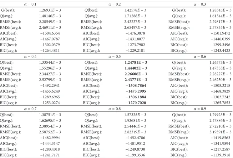
Table 2: Best and average values of𝑄, RMSE, AIC, and BIC fitting errors of the third example for different values of 𝛼 from 0.1 to 0.9 (best results are highlighted in bold).
𝛼 = 0.1 𝛼 = 0.2 𝛼 = 0.3
𝑄(best): 1.26931𝐸 − 3 𝑄(best): 1.42578𝐸 − 3 𝑄(best): 1.28343𝐸 − 3 𝑄(avg.): 1.48146𝐸 − 3 𝑄(avg.): 1.71288𝐸 − 3 𝑄(avg.): 1.61544𝐸 − 3 RMSE(best): 2.28549𝐸 − 3 RMSE(best): 2.42227𝐸 − 3 RMSE(best): 2.29817𝐸 − 3 RMSE(avg.): 2.46911𝐸 − 3 RMSE(avg.): 2.65497𝐸 − 3 RMSE(avg.): 2.57835𝐸 − 3 AIC(best): −1504.6354 AIC(best): −1476.3878 AIC(best): −1501.9472 AIC(avg.): −1467.0787 AIC(avg.): −1431.8077 AIC(avg.): −1446.0399 BIC(best): −1302.0379 BIC(best): −1273.7902 BIC(best): −1299.3496 BIC(avg.): −1264.4811 BIC(avg.): −1229.2101 BIC(avg.): −1243.4423
𝛼 = 0.4 𝛼 = 0.5 𝛼 = 0.6
𝑄(best): 1.33544𝐸 − 3 𝑄(best): 1.24781E − 3 𝑄(best): 1.26573𝐸 − 3 𝑄(avg.): 1.55296𝐸 − 3 𝑄(avg.): 1.44402E − 3 𝑄(avg.): 1.47353𝐸 − 3 RMSE(best): 2.34427𝐸 − 3 RMSE(best): 2.26606E − 3 RMSE(best): 2.28227𝐸 − 3 RMSE(avg.): 2.52799𝐸 − 3 RMSE(avg.): 2.43771E − 3 RMSE(avg.): 2.46250𝐸 − 3 AIC(best): −1492.2941 AIC(best): −1508.7864 AIC(best): −1505.3218 AIC(avg.): −1455.6249 AIC(avg.): −1473.2995 AIC(avg.): −1468.3829 BIC(best): −1289.6965 BIC(best): −1306.1884 BIC(best): −1302.7242 BIC(avg.): −1253.0274 BIC(avg.): −1270.7020 BIC(avg.): −1265.7853
𝛼 = 0.7 𝛼 = 0.8 𝛼 = 0.9
𝑄(best): 1.38751𝐸 − 3 𝑄(best): 1.57325𝐸 − 3 𝑄(best): 1.79923𝐸 − 3 𝑄(avg.): 1.62695𝐸 − 3 𝑄(avg.): 1.93681𝐸 − 3 𝑄(avg.): 2.47886𝐸 − 3 RMSE(best): 2.38954𝐸 − 3 RMSE(best): 2.54446𝐸 − 3 RMSE(best): 2.72210𝐸 − 3 RMSE(avg.): 2.58752𝐸 − 3 RMSE(avg.): 2.82319𝐸 − 3 RMSE(avg.): 3.19391𝐸 − 3 AIC(best): −1482.9994 AIC(best): −1452.4706 AIC(best): −1419.8563 AIC(avg.): −1444.3147 AIC(avg.): −1401.9512 AIC(avg.): −1341.9894 BIC(best): −1280.4018 BIC(best): −1249.8730 BIC(best): −1217.2587 BIC(avg.): −1241.7171 BIC(avg.): −1199.3536 BIC(avg.): −1139.3918
To this purpose, we carried out several simulation trials and computed the fitting error for the eight error criteria used in this work. In this section, we show the results obtained for the first and third examples of this paper.Results for the second example are not reported here because the low number of input data points makes it particularly resilient to variations of parameter 𝛼. As a result, the fitting errors for different values of𝛼 are very similar to each other and to those reported in the second row ofTable 2.
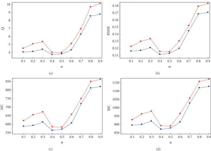
Table 1shows the variation of the eight fitting error crite-ria for the RC circuit example and parameter𝛼 varying from 0.1 to 0.9 with step-size 0.1. Once again, we carried out 20 independent simulations for each value of𝛼 and obtained the best and the average values of the 20 executions. Best results for each error criterion are highlighted in bold for the sake of clarity. We can see that the values𝛼 = 0.4 and 𝛼 = 0.5 lead to the best results for the best and average fitting error values, respectively.Figure 4shows graphically, from left to right and top to bottom, the best (in blue) and average (in red) values of the𝑄, RMSE, AIC, and BIC fitting errors, respectively. From the figure, we can conclude that both𝛼 = 0.4 and 𝛼 = 0.5 are good choices, as they lead to the best results for this example. Note that values lower and larger than this optimal values yield worse fitting error results. This effect is particularly noticeable for values of𝛼 approaching to 1.
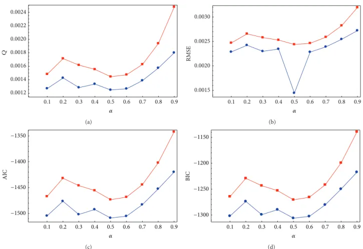
Table 2andFigure 5show the corresponding results for the side profile section of a car body example. As the reader can see, the value 𝛼 = 0.5 is again a very good choice, although𝛼 = 0.1 and 𝛼 = 0.6 also yields good results. Once again, increasing the value of𝛼 towards 1 leads to a strong increase of the fitting errors.
It is worthwhile to recall that the choice of parameters is problem-dependent, meaning that our choice of parameters might not be adequate for other examples. Therefore, it is always advisable to carry out a preliminary analysis and com-puter simulations to determine a proper parameter tuning for better performance, as it has been done in this section.
6.5. Computational Issues. All computations in this paper
have been performed on a 2.9 GHz. Intel Core i7 processor with 8 GB of RAM. The source code has been implemented by the authors in the native programming language of the popular scientific program Matlab, version 2010b. Regarding the computation times, all examples we tested can be obtained in less than a second (excluding rendering). Obviously, the CPU time depends on several factors, such as the number of data points and the values of the different parameters of the method, making it hard to determine how long does it take for a given example to be reconstructed.
0.1 0.2 0.3 0.4 0.5 0.6 0.7 0.8 0.9 4 5 6 7 8 9 10 Q 𝛼 (a) 0.1 0.2 0.3 0.4 0.5 0.6 0.7 0.8 0.9 0.11 0.12 0.13 0.14 0.15 0.16 0.17 0.18 RMS E 𝛼 (b) 0.1 0.2 0.3 0.4 0.5 0.6 0.7 0.8 0.9 550 600 650 700 750 800 850 AI C 𝛼 (c) 0.1 0.2 0.3 0.4 0.5 0.6 0.7 0.8 0.9 850 900 950 1000 1050 1100 1150 BI C 𝛼 (d)
Figure 4: (𝑙-𝑟, 𝑡-𝑏) Variation with parameter 𝛼 of the best (in blue) and average (in red) 𝑄, RMSE, AIC, and BIC fitting error values for the RC circuit example.
7. Comparison with Other Approaches
In this section a careful comparison of our method with other alternative methods is presented. In particular, we compare the results of our method with the two most popular and widely used methods: the uniform and the de Boor methods [28, 29, 32]. These methods differ in the way components of the knot vector are chosen. The uniform method yields equally spaced internal knots as
𝑢𝑗= 𝑗 − 𝑘 + 1𝑛 − 𝑘 + 2, 𝑗 = 𝑘, . . . , 𝑛. (11) This knot vector is simple but does not reflect faithfully the distribution of points. To overcome this problem, a very popular choice is given by the de Boor method as
𝑢𝑗 = (1 − 𝜆𝑗) 𝑡𝑖−1+ 𝜆𝑗𝑡𝑖, 𝑗 = 𝑘, . . . , 𝑛, (12) where𝑑 = 𝑁/(𝑛 − 𝑘 + 2) and 𝜆𝑗 = 𝑗𝑑 − int(𝑗𝑑). Finally, in our method the knots are determined by the best solution of the optimization problem described inSection 3.2, solved with the firefly-based approach described inSection 5. In this section we have applied these three methods to the three examples of this paper.
Table 3summarizes our main results. The three examples analyzed are arranged in rows with the results for each exam-ple in different columns for the compared methods: uniform method, de Boor method, and our method, respectively. For each combination of example and method, eight different fitting errors are reported, corresponding to the best and average value of the𝑄, RMSE, AIC, and BIC error criteria. As mentioned above, the average value is computed from a total of 20 executions for each simulation. The best result for each error criterion is highlighted in bold for the sake of clarity.
It is important to remark here that the error criteria used in this paper for comparison must be carefully analyzed. While the general rule for them is “the lower and the better,” this is exclusively true to compare results obtained for experiments carried out under the same conditions, meaning that we cannot compare the results for the three examples globally, as they are not done under the same conditions (for instance, they have different number of data points, control points, and even the order of the curve). Therefore, we cannot conclude that the fitting curve for the third example (with the lower global AIC/BIC) fits better than the other ones. The only feasible comparison is among the different methods for the same curve under the same simulation conditions. Having said that, some important conclusions can be derived from the numerical results reported inTable 3.
Table 3: Best and average values of𝑄, RMSE, AIC, and BIC fitting errors for the examples in this paper for the uniform method, de Boor method, and our method (best results are highlighted in bold).
Uniform de Boor Our method
RC circuit
𝑄(best): 10.93778001 𝑄(best): 10.19525052 𝑄(best): 3.84178962
𝑄(avg.): 11.73847555 𝑄(avg.): 11.05389142 𝑄(avg.): 4.00119535
RMSE(best): 0.19062565 RMSE(best): 0.18404147 RMSE(best): 0.11297531 RMSE(avg.): 0.19747976 RMSE(avg.): 0.19163478 RMSE(avg.): 0.11529530 AIC(best): 886.05907876 AIC(best): 864.89851523 AIC(best): 571.12743013 AIC(avg.): 907.32445861 AIC(avg.): 889.23754197 AIC(avg.): 583.36453972 BIC(best): 1193.74923073 BIC(best): 1172.58866720 BIC(best): 878.81758210 BIC(avg.): 1215.01461058 BIC(avg.): 1196.92769387 BIC(avg.): 891.05469169
Volumetric moisture content
𝑄(best): 0.00235781 𝑄(best): 0.00012203 𝑄(best): 0.00008527
𝑄(avg.): 0.00476785 𝑄(avg.): 0.00024751 𝑄(avg.): 0.00013525
RMSE(best): 0.01213932 RMSE(best): 0.00276171 RMSE(best): 0.00230860 RMSE(avg.): 0.01726240 RMSE(avg.): 0.00393317 RMSE(avg.): 0.00290751 AIC(best): −72.80034161 AIC(best): −120.17949976 AIC(best): −125.91417106 AIC(avg.): −61.53376508 AIC(avg.): −108.86443657 AIC(avg.): −118.53321768 BIC(best): −63.52927694 BIC(best): −110.90843509 BIC(best): −116.64310640 BIC(avg.): −52.26270041 BIC(avg.): −99.59337190 BIC(avg.): −109.26215301
Side profile of car body
𝑄(best): 0.00647026 𝑄: 0.00280562 𝑄(best): 0.00124781
𝑄(avg.): 0.00738719 𝑄(avg.): 0.00310424 𝑄(avg.): 0.00144402
RMSE(best): 0.00516009 RMSE(best): 0.00339791 RMSE(best): 0.00226606 RMSE(avg.): 0.00551361 RMSE(avg.): 0.00357416 RMSE(avg.): 0.00243771 AIC(best): −1108.85088744 AIC(best): −1311.89939612 AIC(best): −1508.78640537 AIC(avg.): −1076.64583126 AIC(avg.): −1287.32145345 AIC(avg.): −1473.29956438 BIC(best): −906.25332372 BIC(best): −1109.30183241 BIC(best): −1306.18841665 BIC(avg.): −874.04826754 BIC(avg.): −1084.72388973 BIC(avg.): −1270.70200066
(i) First and foremost, they confirm the good results of our method for the examples discussed in this paper. The fitting errors are very low in all cases, meaning that the fitting curve approximates the given data very accurately.
(ii) On the other hand, the numerical results clearly show that our method outperforms the most popular alter-native methods in all cases. The proposed approach provides the best results for all error criteria and for all examples, both for the best and for the average values. (iii) Note also that the uniform approach is the worst in all examples, as expected because of its inability to account for the distribution of data points of the given problem. This problem is partially alleviated by the de Boor approach but the errors can still be further improved. This is what our method actually does. To summarize, the numerical results from our exper-iments confirms the very accurate fitting to data points obtained with the proposed method as well as its superiority over the most popular alternatives in the field. This superior performance can be explained from a theoretical point of view. Firstly, we notice that the uniform method does not reflect the real distribution of points; in fact, (11) shows that the knots depend exclusively on 𝑛 and 𝑘, and hence it is independent of the input data. Consequently, it lacks the ability to adapt to the shape of the underlying function of data.
Regarding the de Boor method, the choice of knots is based on ensuring that the system of equations is well conditioned and has solution on optimizing the process. Accordingly, it focuses on the numerical properties of the matrices involved. From (4) and (5), we can obtain the following vector equation:
Y = N ⋅ B, (13)
whereY = (𝑦1, 𝑦2, . . . , 𝑦𝑁)𝑇and𝑁 = ({𝑁𝑗,𝑘(𝑡𝑖)}𝑗=0,...,𝑛;𝑖=1,...,𝑁) is the matrix of basis functions sampled at data point parameters. Premultiplying at both sides byN𝑇, we obtain
N𝑇⋅ Y = N𝑇⋅ N ⋅ B, (14)
where N𝑇 ⋅ N is a real symmetric matrix and, therefore, Hermitian, so all its eigenvalues are real. In fact, up to a choice of an orthonormal basis, it is a diagonal matrix, whose diagonal entries are the eigenvalues. It is also a positive semidefinite matrix, so the system has always solution. It can be proved that the knots in the de Boor method are chosen so that it is guaranteed that every knot span contains at least one parametric value [59]. This condition implies that theN𝑇⋅N is positive definite and well conditioned. As a consequence, the system (14) is nonsingular and can be solved by computing the inverse of matrix N𝑇 ⋅ N. As the reader can see, the choice of knots in this method is motivated by the numerical
0.1 0.2 0.3 0.4 0.5 0.6 0.7 0.8 0.9 0.0012 0.0014 0.0016 0.0018 0.0020 0.0022 0.0024 Q 𝛼 (a) 0.1 0.2 0.3 0.4 0.5 0.6 0.7 0.8 0.9 0.0015 0.0020 0.0025 0.0030 RMS E 𝛼 (b) 0.1 0.2 0.3 0.4 0.5 0.6 0.7 0.8 0.9 AI C −1500 −1450 −1400 −1350 𝛼 (c) 0.1 0.2 0.3 0.4 0.5 0.6 0.7 0.8 0.9 BI C −1300 −1250 −1200 −1150 𝛼 (d)
Figure 5: (𝑙-𝑟, 𝑡-𝑏) Variation with parameter 𝛼 of the best (in blue) and average (in red) 𝑄, RMSE, AIC, and BIC fitting error values for the RC circuit example.
properties of matrixN, and never attempted to formulate the fitting process as an optimization problem. In clear contrast, in our approach the problem is formulated as an optimization problem, given by minimize {𝑢𝑙}𝑙=𝑘,...,𝑛 {𝑏𝑗}𝑗=0,...,𝑛 { { { 𝑁 ∑ 𝑖=1 (𝑦𝑖−∑𝑛 𝑗=0 𝑁𝑗,𝑘(𝑡𝑖) 𝑏𝑗) 2 } } } . (15)
In other words, in our method the emphasis is on optimizing the choice of knots rather than on the numerical properties of the system equation. Note that our method allows con-secutive nodes to be as close as necessary; they can even be equal. A simple visual inspection of (11) and (12) shows that this choice is not allowed in these alternative methods. However, near knots are sometimes required for very steep upwards/downwards areas or areas of sharp changes of concavity, such as those in the figures of this paper. These facts justify why our method outperforms both the uniform and the de Boor methods for the computation of the knot vector.
8. Conclusions and Future Work
This paper addresses the problem of curve fitting to noisy data points by using explicit B-spline curves. Given a set of noisy data points, the goal is to compute all parameters of the approximating explicit polynomial B-spline curve that best fits the set of data points in the least-squares sense. This is a very difficult overdetermined, continuous, multimodal, and multivariate nonlinear optimization problem. Our pro-posed method solves it by applying the firefly algorithm, a powerful metaheuristic nature-inspired algorithm well suited for optimization. The method has been applied to three illustrative real-world engineering examples from different fields. Our experimental results show that the presented method performs very well, being able to fit the data points with a high degree of accuracy. A comparison with the most popular previous approaches to this problem is also carried out. It shows that our method outperforms previous approaches for the examples discussed in this paper for eight different fitting error criteria.
Future work includes the extension of this method to other families of curves, such as the parametric B-spline curves and NURBS. The extension of these results to the case of explicit surfaces is also part of our future work. Finally, we
are also interested to apply our methodology to other real-world problems of interest in industrial environments.
Acknowledgments
This research has been kindly supported by the Computer Science National Program of the Spanish Ministry of Econ-omy and Competitiveness, Project Ref. no. TIN2012-30768, Toho University (Funabashi, Japan), and the University of Cantabria (Santander, Spain). The authors are particularly grateful to the Department of Information Science of Toho University for all the facilities given to carry out this research work. Special thanks are owed to the Editor and the anony-mous reviewers for their useful comments and suggestions that allowed us to improve the final version of this paper.
References
[1] P. Gu and X. Yan, “Neural network approach to the reconstruc-tion of freeform surfaces for reverse engineering,” Computer
Aided Design, vol. 27, no. 1, pp. 59–64, 1995.
[2] W. Ma and J. Kruth, “Parameterization of randomly measured points for least squares fitting of B-spline curves and surfaces,”
Computer Aided Design, vol. 27, no. 9, pp. 663–675, 1995.
[3] A. Iglesias and A. G´alvez, “A new artificial intelligence paradigm for computer aided geometric design,” in Artificial Intelligence
and Symbolic Computation, vol. 1930 of Lectures Notes in Artificial Intelligence, pp. 200–213, 2001.
[4] A. Iglesias and A. G´alvez, “Applying functional networks to fit data points from B-spline surfaces,” in Proceedings of the
Computer Graphics International (CGI ’01), pp. 329–332, IEEE
Computer Society Press, Hong Kong, 2001.
[5] G. Echevarr´ıa, A. Iglesias, and A. G´alvez, “Extending neural net-works for B-spline surface reconstruction,” in Computational
Science, vol. 2330 of Lectures Notes in Computer Science, pp. 305–
314, 2002.
[6] H. Yang, W. Wang, and J. Sun, “Control point adjustment for B-spline curve approximation,” Computer Aided Design, vol. 36, no. 7, pp. 639–652, 2004.
[7] A. Iglesias, G. Echevarr´ıa, and A. G´alvez, “Functional networks for B-spline surface reconstruction,” Future Generation
Com-puter Systems, vol. 20, no. 8, pp. 1337–1353, 2004.
[8] M. Hoffmann, “Numerical control of Kohonen neural network for scattered data approximation,” Numerical Algorithms, vol. 39, no. 1–3, pp. 175–186, 2005.
[9] W. P. Wang, H. Pottmann, and Y. Liu, “Fitting B-spline curves to point clouds by curvature-based squared distance minimiza-tion,” ACM Transactions on Graphics, vol. 25, no. 2, pp. 214–238, 2006.
[10] A. G´alvez, A. Cobo, J. Puig-Pey, and A. Iglesias, “Particle swarm optimization for B´ezier surface reconstruction,” in
Computa-tional Science, vol. 5102 of Lectures Notes in Computer Science,
pp. 116–125, 2008.
[11] X. Zhao, C. Zhang, B. Yang, and P. Li, “Adaptive knot placement using a GMM-based continuous optimization algorithm in B-spline curve approximation,” Computer Aided Design, vol. 43, no. 6, pp. 598–604, 2011.
[12] A. G´alvez, A. Iglesias, and J. Puig-Pey, “Iterative two-step genetic-algorithm-based method for efficient polynomial B-spline surface reconstruction,” Information Sciences, vol. 182, no. 1, pp. 56–76, 2012.
[13] A. G´alvez and A. Iglesias, “Particle swarm optimization for non-uniform rational B-spline surface reconstruction from clouds of 3D data points,” Information Sciences, vol. 192, pp. 174–192, 2012. [14] A. G´alvez and A. Iglesias, “Firefly algorithm for polynomial B´ezier surface parameterization,” Journal of Applied
Mathemat-ics, Article ID 237984, 9 pages, 2013.
[15] N. M. Patrikalakis and T. Maekawa, Shape Interrogation for
Computer Aided Design and Manufacturing, Springer, Berlin,
Germany, 2002.
[16] H. Pottmann, S. Leopoldseder, M. Hofer, T. Steiner, and W. Wang, “Industrial geometry: recent advances and applications in CAD,” Computer Aided Design, vol. 37, no. 7, pp. 751–766, 2005.
[17] T. C. M. Lee, “On algorithms for ordinary least squares regres-sion spline fitting: a comparative study,” Journal of Statistical
Computation and Simulation, vol. 72, no. 8, pp. 647–663, 2002.
[18] H. Park, “An error-bounded approximate method for repre-senting planar curves in B-splines,” Computer Aided Geometric
Design, vol. 21, no. 5, pp. 479–497, 2004.
[19] L. Jing and L. Sun, “Fitting B-spline curves by least squares sup-port vector machines,” in Proceedings of the 2nd International
Conference on Neural Networks and Brain (ICNNB ’05), pp. 905–
909, IEEE Press, October 2005.
[20] W. Li, S. Xu, G. Zhao, and L. P. Goh, “Adaptive knot placement in B-spline curve approximation,” Computer Aided Design, vol. 37, no. 8, pp. 791–797, 2005.
[21] A. G´alvez, A. Iglesias, A. Cobo, J. Puig-Pey, and J. Espinola, “B´ezier curve and surface fitting of 3D point clouds through genetic algorithms, functional networks and least-squares approximation,” in Computational Science and Its Applications, vol. 4706 of Lectures Notes in Computer Science, pp. 680–693, 2007.
[22] H. Park and J.-H. Lee, “B-spline curve fitting based on adaptive curve refinement using dominant points,” Computer Aided
Design, vol. 39, no. 6, pp. 439–451, 2007.
[23] A. Iglesias and A. G´alvez, “Curve fitting with RBS functional networks,” in Proceedings of the International Conference on
Convergence Information Technology (ICCIT ’08), vol. 1, pp.
299–306, IEEE Computer Society Press, Busan, Republic of Korea, 2008.
[24] A. G´alvez and A. Iglesias, “Efficient particle swarm optimization approach for data fitting with free knot B-splines,” Computer
Aided Design, vol. 43, no. 12, pp. 1683–1692, 2011.
[25] A. G´alvez, A. Iglesias, and A. Andreina, “Discrete B´ezier curve fitting with artificial immune systems,” Studies in
Computa-tional Intelligence, vol. 441, pp. 59–75, 2013.
[26] A. G´alvez and A. Iglesias, “A new iterative mutually-coupled hybrid GA-PSO approach for curve fitting in manufacturing,”
Applied Soft Computing, vol. 13, no. 3, pp. 1491–1504, 2013.
[27] R. E. Barnhill, Geometry Processing for Design and
Manufactur-ing, Society for Industrial and Applied Mathematics (SIAM),
Philadelphia, Pa, USA, 1992.
[28] J. Hoschek and D. Lasser, Fundamentals of Computer Aided
Geometric Design, A K Peters, Wellesley, Mass, USA, 1993.
[29] G. Farin, Curves and Surfaces for CAGD, Morgan Kaufmann, San Francisco, Calif, USA, 5th edition, 2002.
[30] J. R. Rice, The Approximation of Functions. Vol. 2: Nonlinear
and Multivariate Theory, Addison-Wesley, Reading, Mass, USA,
1969.
[31] D. L. B. Jupp, “Approximation to data by splines with free knots,”
SIAM Journal on Numerical Analysis, vol. 15, no. 2, pp. 328–343,
[32] L. Piegl and W. Tiller, The NURBS Book, Springer, Berlin, Germany, 1997.
[33] T. V´arady, R. R. Martin, and J. Cox, “Reverse engineering of geometric models: an introduction,” Computer Aided Design, vol. 29, no. 4, pp. 255–268, 1997.
[34] T. Varady and R. Martin, “Reverse engineering,” in Handbook
of Computer Aided Geometric Design, G. Farin, J. Hoschek, and
M. Kim, Eds., pp. 651–681, Elsevier, 2002.
[35] C. A. de Boor and J. R. Rice, Least Squares Cubic Spline
Approximation. I: Fixed Knots, CSD TR 20, Purdue University,
Lafayette, Ind, USA, 1968.
[36] C. A. de Boor and J. R. Rice, Least Squares Cubic Spline
Approx-imation. II: Variable Knots, CSD TR 21, Purdue University,
Lafayette, Ind, USA, 1968.
[37] H. G. Burchard, “Splines (with optimal knots) are better,”
Applicable Analysis, vol. 3, pp. 309–319, 1974.
[38] C. A. de Boor, A Practical Guide to Splines, vol. 27, Springer, New York, NY, USA, 2001.
[39] T. Lyche and K. Mørken, “Knot removal for parametric𝐵-spline curves and surfaces,” Computer Aided Geometric Design, vol. 4, no. 3, pp. 217–230, 1987.
[40] T. Lyche and K. Mørken, “A data-reduction strategy for splines with applications to the approximation of functions and data,”
IMA Journal of Numerical Analysis, vol. 8, no. 2, pp. 185–208,
1988.
[41] P. Dierckx, Curve and Surface Fitting with Splines, Oxford University Press, Oxford, UK, 1993.
[42] M. Alhanaty and M. Bercovier, “Curve and surface fitting and design by optimal control methods,” Computer Aided Design, vol. 33, no. 2, pp. 167–182, 2001.
[43] R. Goldenthal and M. Bercovier, “Spline curve approximation and design by optimal control over the knots,” Computing, vol. 72, no. 1-2, pp. 53–64, 2004.
[44] M. J. D. Powell, “Curve fitting by splines in one variable,” in
Numerical Approximation To Functions and Data, J. G. Hayes,
Ed., Athlone Press, London, UK, 1970.
[45] M. Crampin, R. Guifo Guifo, and G. A. Read, “Linear approxi-mation of curves with bounded curvature and a data reduction algorithm,” Computer-Aided Design, vol. 17, no. 6, pp. 257–261, 1985.
[46] G. E. H¨olzle, “Knot placement for piecewise polynomial approx-imation of curves,” Computer Aided Design, vol. 15, no. 5, pp. 295–296, 1983.
[47] L. A. Piegl and W. Tiller, “Least-squares B-spline curve approx-imation with arbitrary end derivatives,” Engineering with
Com-puters, vol. 16, no. 2, pp. 109–116, 2000.
[48] E. Castillo and A. Iglesias, “Some characterizations of families of surfaces using functional equations,” ACM Transactions on
Graphics, vol. 16, no. 3, pp. 296–318, 1997.
[49] F. Yoshimoto, M. Moriyama, and T. Harada, “Automatic knot adjustment by a genetic algorithm for data fitting with a spline,” in Proceedings of the Shape Modeling International, pp. 162–169, IEEE Computer Society Press, 1999.
[50] M. Sarfraz and S. A. Raza, “Capturing outline of fonts using genetic algorithms and splines,” in Proceedings of the 5th
International Conference on Information Visualization (IV ’01),
pp. 738–743, IEEE Computer Society Press, 2001.
[51] F. Yoshimoto, T. Harada, and Y. Yoshimoto, “Data fitting with a spline using a real-coded genetic algorithm,” Computer Aided
Design, vol. 35, no. 8, pp. 751–760, 2003.
[52] E. ¨Ulker and A. Arslan, “Automatic knot adjustment using an artificial immune system for B-spline curve approximation,”
Information Sciences, vol. 179, no. 10, pp. 1483–1494, 2009.
[53] X.-S. Yang, “Firefly algorithms for multimodal optimization,” in Stochastic algorithms: foundations and applications, vol. 5792 of Lectures Notes in Computer Science, pp. 169–178, Springer, Berlin, Germany, 2009.
[54] X. S. Yang, “Firefly algorithm, stochastic test functions and design optimisation,” International Journal of Bio-Inspired
Com-putation, vol. 2, no. 2, pp. 78–84, 2010.
[55] H. Akaike, “Information theory and an extension of the maximum likelihood principle,” in Proceedings of the 2nd
International Symposium on Information Theory, B. N. Petrov
and F. Csaki, Eds., pp. 267–281, Akad´emiai Kiad´o, Budapest, Hungary, 1973.
[56] H. Akaike, “A new look at the statistical model identification,”
IEEE Transactions on Automatic Control, vol. 19, no. 6, pp. 716–
723, 1974.
[57] G. Schwarz, “Estimating the dimension of a model,” The Annals
of Statistics, vol. 6, no. 2, pp. 461–464, 1978.
[58] “Volvo Car Coordinate. Volvo Cars Report,” 2009.
[59] C. A. de Boor, Practical Guide to Splines, Springer, 2nd edition, 2001.
Impact Factor 1.730
28 Days
Fast Track Peer Review
All Subject Areas of Science
Submit at http://www.tswj.com
Hindawi Publishing Corporationhttp://www.hindawi.com Volume 2013
Hindawi Publishing Corporation
http://www.hindawi.com Volume 2013