Thermo hydraulic performance modeling of thermal energy systems using parabolic trough solar collectors

Texto completo

(1)Instituto Tecnológico y de Estudios Superiores de Monterrey Campus Monterrey. School of Engineering and Sciences. Thermo-hydraulic performance modeling of thermal energy systems using parabolic trough solar collectors A dissertation presented by. Pablo Daniel Tagle Salazar Submitted to the School of Engineering and Sciences in partial fulfillment of the requirements for the degree of Doctor of Philosophy In Engineering Science. Major in Environmental Systems and Energy. Monterrey Nuevo León, December 26th, 2018.

(2)

(3)

(4) @2018 by Pablo Daniel Tagle Salazar All rights reserved. Dedication In memoriam of my father, Arnoldo, and in honor to my mother, Julia. For my professors, the ones who has forged my identity. For my friends, the people who was there, everyone who is here now, and the ones who will come.. iii.

(5) Acknowledgements The author acknowledges to all professors of Tecnologico de Monterrey who contributed with this research and the support of the Energy and Climate Change Research Group. I would like to acknowledge to CONACYT for support for living. I also would like to express my gratitude to the staff from Plataforma Solar de Almeria for their support and collaboration during my research internship, in special to Loreto Valenzuela.. iv.

(6) Thermo-hydraulic performance modeling of thermal energy systems using parabolic trough solar collectors By Pablo Daniel Tagle Salazar. Abstract Solar energy is one of the most important emerging renewable energy resources. Parabolic trough solar collectors are one of the most used technologies for solar concentrating applications. The main purpose of this research is to develop a mathematical model for predicting thermodynamics and hydraulics of solar-to-heat conversion of thermal systems using parabolic trough collectors. Thermal model is based on energy balance of a one-dimensional steady-state heat transfer thermal resistance circuit. The receiver and its surroundings are considered as the control volume of the analysis. Heat transfer coefficients are obtained using experimental correlations found in the literature. The model considers single-phase and two-phase flow with phase-change effects, where pressure drop is solved simultaneously with thermal energy balance. The input data corresponds to optics properties, design of collector, weather data, and basic hydraulic parameters (for series or parallel configurations). Parabolic trough collectors with Al2O3/water nanofluid is also considered as a case of study. Computational simulations are carried out using Engineering Equation Solver (EES), a software developed to solve complex systems of non-linear equations. This software was selected due to its simplicity in programing systems of non-linear equations and the available database of thermophysical properties of number of substances, including water and steam. Experimental data is used to validate the model, comparing with simulation results. Simulations are realized using same ambient and inlet operational conditions as described in test results. Sources of experimental data are test results of four collectors (for efficiency curves case), a M.Sc. Thesis previously presented (for nanofluid case), and from data provided by Plataforma Solar de Almeria (for direct steam generation case). Results show a good agreement between simulations and experiments. Thermal parameters (such as thermal efficiency and temperatures) are predicted with high accuracy. There was obtained a global absolute error of around 1.5 °C for temperatures and 2% in thermal efficiency. Comparison of temperature and pressure profiles using simulation results and experimental data of a direct steam generation system in oncetrough mode show that the model can predict phase-change phenomena with high accuracy. Although, the model fails in predicting pressure drop with high steam quality two-phase flow.. v.

(7) List of Figures Fig. 2.1 – Classification of solar energy technologies.................................................... 18 Fig. 2.2 – Parabolic Trough Solar Collector................................................................... 21 Fig. 2.3 – Geometrical errors in mirrors ......................................................................... 22 Fig. 2.4 – PTC solar receiver ......................................................................................... 24 Fig. 2.5 – Operation of active trackers. a) closed-loop, b) open-loop. ........................... 29 Fig. 2.6 – Temperature range of some potential thermal applications for PTCs ............ 30 Figure 2.7 - CSP plant diagrams a) Direct SG, b) Indirect SG integrated to a combined cycle. ............................................................................................................................. 31 Fig. 2.8 – Absorption solar cooling systems. a) single effect, b) double effect .............. 33 Fig. 2.9 – Adsorption solar cooling system .................................................................... 33 Fig. 2.10 – Evolution of solar cell technology. Borrowed from NREL website (www.nrel.gov/pv).......................................................................................................... 37 Fig. 2.11 – Classification of thermal performance analysis. .......................................... 38 Fig. 2.11 – Definition of acceptance angle .................................................................... 42 Fig. 2.12 – Geometry of a PTC ..................................................................................... 42 Fig. 2.13 – Description of end-effect losses .................................................................. 43 Fig. 2.14 – Thermal efficiency curve and components of heat losses ........................... 44 Fig. 3.1 - Boundary of the analysis of the collector ........................................................ 57 Fig. 3.2 - Thermal resistance model for the receiver ..................................................... 58 Fig. 3.3 - Energy balance around the fluid..................................................................... 59 Fig. 3.4 - Thermal resistance model for interconnecting piping ..................................... 62 Fig. 3.5 - Energy balance around the interconnecting piping ........................................ 62 Fig. 3.6 - Nu vs. Re for single-phase internal forced convection (Pr=0.7, Pr/Prw=1). .... 63 Fig. 3.7 - f vs. Re for single-phase flow ......................................................................... 64 Fig. 3.8 - Typical flow pattern map for two-phase flow .................................................. 67 Fig. 3.9 – Behavior of flow patterns ............................................................................... 67 Fig. 3.10 - Flowchart algorithm ...................................................................................... 68 Fig. 3.11 – Thermo-hydraulic parameters vs. quality in two-phase phenomena ........... 70 Fig. 3.12 – Temperature vs. entropy diagrams for phase change phenomena ............. 72 Fig. 3.13 – Nu vs. Re for internal forced convection using Al2O3/water nanofluid (Pr/Prw=1) ...................................................................................................................... 74 Fig. 3.14 – Inputs for ambient conditions of collector system ........................................ 77. vi.

(8) Fig. 3.15 – Inputs for collector design used in thermal analysis .................................... 78 Fig. 3.16 – Inputs for system description section. ......................................................... 79 Fig. 3.17 – Defining variable limits ................................................................................ 79 Fig. 3.18 – Warning message for convergence ............................................................. 80 Fig. 3.19 – Temperature, pressure and quality of steam profiles. ................................. 80 Fig. 4.1 – Efficiency curve for LS-2 with PTR-70 receiver ............................................. 88 Fig. 4.2 – Comparison of output parameters for LS-2 with PTR-70 receiver ................. 88 Fig. 4.3 – Absolute errors’ boxplots of output parameters for LS-2 with PTR-70 receiver ...................................................................................................................................... 89 Fig. 4.4 – Efficiency curve for LS-2 using UVAC receiver and Cermet coating ............. 90 Fig. 4.5 – Efficiency curve for LS-2 using UVAC receiver and Black Chrome coating .. 90 Fig. 4.6 – Comparison of output parameters for LS-2 using UVAC receiver and Cermet coating........................................................................................................................... 91 Fig. 4.7 – Comparison of output parameters for LS-2 using UVAC receiver and Black Chrome coating ............................................................................................................. 91 Fig. 4.8 – Absolute errors’ boxplots of output parameters for LS-2 with UVAC receiver and Cermet coating. a) Air in annulus, b) Vacuum in annulus. ...................................... 92 Fig. 4.9 – Absolute errors’ boxplots of output parameters for LS-2 with UVAC receiver and Black Chrome coating. a) Air in annulus, b) Vacuum in annulus. ........................... 92 Fig. 4.10 – Efficiency curve for URSSA Trough PTC .................................................... 94 Fig. 4.11 – Comparison of output parameters for URSSA Trough ................................ 95 Fig. 4.12 – Absolute errors’ boxplots of output parameters for URSSA Trough ............ 95 Figure 4.13 – Efficiency curve of CAPSOL PTC ........................................................... 96 Fig. 4.14 – Comparison of output parameters for CAPSOL .......................................... 97 Fig. 4.15 – Absolute errors’ boxplots of output parameters for CAPSOL ...................... 97 Fig 4.16 – Hydraulic diagram for experimental tests with nanofluids. ............................ 98 Fig. 4.17 – Efficiency curve of experiments and simulations for the Al2O3-water nanofluid with 1% of volume concentration ................................................................. 100 Fig. 4.18 – Schematic diagram of DISS facility loop (PSA). ........................................ 101 Fig. 4.19 – Operational conditions of the DISS plant at 2/April/2001 ........................... 103 Fig. 4.20 - Operational conditions of the DISS plant at 13/May/2001 .......................... 104 Fig. 4.21 – Operational conditions of the DISS plant at 15/May/2001 ......................... 105 Fig. 4.22 – Comparison of simulated and experimental temperature / pressure profiles (2/Apr). a) 16h, b) 17h, c) 18h ..................................................................................... 107. vii.

(9) Fig. 4.23 – Comparison of simulated and experimental temperature / pressure profiles (13/May). a) 13.45h, b) 14:30h, c) 15h ........................................................................ 108 Fig. 4.24 – Comparison of simulated and experimental temperature / pressure profiles (15/May). a) 14h, b) 15h .............................................................................................. 109 Fig. 4.25 – Schematic diagram of solar field ............................................................... 110 Fig. 4.26 – Outlet pressure for a flow rate of 9 GPM, inlet pressure of 25 barg, and ambient temperature of 18 °C. .................................................................................... 111 Fig. 4.27 – Selection of operational region of solar field. ............................................. 111 Fig. 4.28 – Level curves for mass flow, thermal power, and over-heating temperature difference. ................................................................................................................... 113 Fig. A.1 – Inlet data in system description section for different types of analysis. a) Single-phase flow without nanofluids, b) Single-phase flow using nanofluids, c) Twophase flow ................................................................................................................... 119 Fig. A.2 – Solution window .......................................................................................... 120 Fig. A.3 – Arrays table ................................................................................................. 120 Figure A.4 – Fixing limits for manual phase-change prediction ................................... 121 Figure A.5 – Error message for manual phase-change prediction .............................. 122 Fig. B.1 – Windows for parametrization. a) selecting the variable, b) deactivating the variable, c) Variable deactivated. ................................................................................ 123 Fig. B.2 – Defining new parametric table..................................................................... 124 Fig. B.3 – New parametric table. a) Table, b) defining values of parametric variables 124. viii.

(10) List of Tables Table 1.1 – Software tools used for analysis with PTCs [8-14] ...................................... 4 Table 1.2 – Studies and models of thermal analysis of PTCs. ........................................ 6 Table 2.1 - Comparison of solar concentrating technologies......................................... 19 Table 2.2 – Advantages and Disadvantages of PTC technology .................................. 21 Table 2.3 - Types of mirrors and their properties .......................................................... 23 Table 2.4 - Characteristics of some receivers available in market ................................ 26 Table 2.5 - Heat transfer fluids used on PTC fields ....................................................... 27 Table 2.6 – Characteristics of concentrating photovoltaic applications ......................... 36 Table 2.7 - Experimental studies of collectors ............................................................... 39 Table 2.8 – Correlations for incidence angle and slope angle of surface for PTC ......... 43 Table 2.9 – Reliability and performance tests included in each standard ...................... 45 Table 3.1 – Heat transfer modes in thermal resistance model ...................................... 59 Table 3.2 - Constants for (3.47) .................................................................................... 66 Table 3.3 - Equations for pressure drop modeling ........................................................ 69 Table 3.4 – Mathematical model for other heat transfer phenomena ............................ 75 Table 3.5 - Constants for Zhukauskas correlation ......................................................... 76 Table 4.1 – Resume of geometrical parameters of simulated collectors ....................... 87 Table 4.2 – Descriptive statistics for absolute errors (LS-2 + PTR-70).......................... 89 Table 4.3 – Descriptive statistics for absolute errors (LS-2 + UVAC and Cermet) ........ 92 Table 4.4 – Descriptive statistics for absolute errors (LS-2 + UVAC and Black Chrome) ...................................................................................................................................... 93 Table 4.5 – Descriptive statistics for absolute errors (URSSA Trough) ......................... 94 Table 4.5 – Descriptive statistics for absolute errors (CAPSOL) ................................... 97 Table 4.6 – Characteristics of PT-110 ........................................................................... 98 Table 4.7 – Experimental and simulation data comparison for the Al2O3-water nanofluid with 1% of volume concentration ................................................................................... 99 Table 4.8 – Coefficients thermal efficiency curve for the Al2O3-water nanofluid with 1% of volume concentration ................................................................................................ 99 Table 4.9 – Descriptive statistics for absolute errors (PT-110 with nanofluid as HTF) 100 Table 4.10 – Characteristics of LS-3 collector ............................................................. 102 Table 4.11 – Steady-state temporal intervals .............................................................. 102 Table 4.12 – Resume of operational conditions for simulations .................................. 106. ix.

(11) Table 4.13 – Error in inlet temperature between experiments and simulations (ºC) .... 106 Table 4.14 – Error in pressure drop between experiments and simulations (barg) ..... 106 Table 4.15 – Statistics of absolute errors .................................................................... 109 Table 4.16 – Characteristics of PT250 collector. ......................................................... 110 Table 4.17 – Variation of outlet conditions. ................................................................. 112. x.

(12) Contents Abstract ........................................................................................................................... v List of Figures ..................................................................................................................vi List of Tables ...................................................................................................................ix Chapter 1. Problem statement ..................................................................................... 1. 1.1 Background .......................................................................................................... 1 1.1.1 Software available in market .......................................................................... 2 1.1.2 Thermal models in the literature ..................................................................... 3 1.2 Problem statement.............................................................................................. 12 1.3 Objectives ........................................................................................................... 12 1.4 Scope ................................................................................................................. 13 1.5 General Assumptions ......................................................................................... 13 1.6 Expected results ................................................................................................. 13 1.7 Nomenclature ..................................................................................................... 14 1.7.1 Acronyms ..................................................................................................... 14 1.8 References ......................................................................................................... 14 Chapter 2. Introduction to Parabolic Trough Technology .......................................... 18. 2.1 A brief description of the Parabolic-Trough collector technology ........................ 18 2.1.1 Background .................................................................................................. 18 2.1.2 Components ................................................................................................. 21 2.1.2.1 Mirrors .................................................................................................... 22 2.1.2.2 Supporting structure ............................................................................... 24 2.1.2.3 Receiver ................................................................................................. 24 2.1.2.4 Heat transfer Fluid ................................................................................. 25 2.1.2.5 Solar tracking system ............................................................................. 25 2.2 Industrial applications ......................................................................................... 30 2.2.1 Heating ......................................................................................................... 30 2.2.2 Cooling ......................................................................................................... 32 2.2.3 Seawater desalination .................................................................................. 34 2.2.4 Water decontamination ................................................................................ 35 2.2.5 Concentrating photovoltaics ......................................................................... 35. xi.

(13) 2.3 Performance analysis methods........................................................................... 36 2.3.1 Thermal performance ................................................................................... 36 2.3.2 Optical performance ..................................................................................... 41 2.4 Basic concepts on performance of Parabolic-Trough collectors ......................... 41 2.4.1 Geometric factors ......................................................................................... 41 2.4.2 Thermal efficiency curve............................................................................... 43 2.5 Nomenclature ..................................................................................................... 47 2.5.1 Acronyms ..................................................................................................... 47 2.5.2 Symbols........................................................................................................ 47 2.5.3 Greek letters ................................................................................................. 48 2.6 References ......................................................................................................... 48 Chapter 3. Description of modeling ........................................................................... 57. Abstract ..................................................................................................................... 57 3.1 Thermo-hydraulic model ..................................................................................... 57 3.1.1 Energy Balance Equations for Receiver ....................................................... 58 3.1.2 Energy Balance Equations for Interconnecting Piping .................................. 61 3.1.3 Single-phase Internal Forced Convection..................................................... 62 3.1.4 Two-phase Internal Forced Convection ........................................................ 64 3.1.5 Modeling phase change phenomena ........................................................... 71 3.1.6 Internal forced convection using Al2O3/water nanofluids .............................. 73 3.1.7 Other Heat Transfer Phenomena ................................................................. 74 3.1.7.1 Natural annular convection .................................................................... 74 3.1.7.2 Natural external convection.................................................................... 74 3.1.7.3 Cross-flow external forced convection ................................................... 76 3.1.7.4 External convection in extended surfaces .............................................. 76 3.1.7.5 Radiation in Annular region .................................................................... 76 3.1.7.6 External radiation ................................................................................... 76 3.2 A brief description of thermal analysis using Engineering Equation Solver ........ 77 3.2.1 Background .................................................................................................. 77 3.2.2 Input data window ........................................................................................ 77 3.2.3 Convergence ................................................................................................ 79 3.2.4 Output data window ...................................................................................... 80 3.3 Nomenclature ..................................................................................................... 80 xii.

(14) 3.4 References ......................................................................................................... 84 Chapter 4. Results and discussion ............................................................................ 86. 4.1 Case 1: Thermal efficiency curves ...................................................................... 86 4.1.1 LS-2 with a PTR-70 receiver ........................................................................ 86 4.1.2 LS-2 with an UVAC receiver ......................................................................... 89 4.1.3 URSSA Trough ............................................................................................. 93 4.1.4 CAPSOL ....................................................................................................... 95 4.2 Case 2: Parabolic trough using nanofluids ......................................................... 97 4.3 Case 3: Direct steam generation ...................................................................... 101 4.4 Case 4: Estimation of thermal power for steam generation in a dairy plant ...... 110 4.5 Nomenclature ................................................................................................... 113 4.6 References ....................................................................................................... 114 Chapter 5. Conclusions ........................................................................................... 116. Conclusions ............................................................................................................. 116 Recommendations ................................................................................................... 117 Future work .............................................................................................................. 117 Appendix A. General user manual of windows in Engineering Equation Solver ..... 119. A.1 Input data window ............................................................................................. 119 A.2 Solution in Single-phase flow ............................................................................ 120 A.3 Solution in two-phase flow ................................................................................ 121 Appendix B. Parametric analysis in Engineering Equation Solver .......................... 123. Published papers ..................................................................................................... 125 Curriculum Vitae .......................................................................................................... 129. xiii.

(15) Chapter 1. Problem statement. The main idea of this chapter is to stablish the general scene of the research. Scope, objectives, and expected results are presented. There is given a brief description of background of previous research and computational tools used to simulate solar conversion systems. The organization of this thesis is also described below. 1.1 Background The penetration of renewable technologies in the international power generation market has increased in recent years all around the world. The principal reason is the growing interest of governments in implementing renewable energy generation systems to mitigate greenhouse gas (GHG) emissions and provide better energy security. At the end of 2015, around 150 countries implemented energy improvement policies, and at least 128 established energy efficiency strategies and targets [1]. One of the most important applications for Parabolic Trough Collector (PTC) technology is electricity generation. The installed capacity of power plants with PTC technology has increased in the last decade, with the United States and Spain being the principal contributors in solar thermal power generation. Most of the electricity generation systems using solar thermal resources are PTC-based, accounting for approximately 85% of total current installed capacity worldwide [2]. In 2014, the demand of thermal energy in industry was around 85.3EJ, equivalent to 74% of industrial energy needs [3]. Near 52% of this demand is applied into low-to-medium temperature heating applications, which shows a high potential of Solar Heating Industrial Processes (SHIPs) for industrial thermal energy supply. PTCs are one of the technologies used in SHIPs that have recently been developed and implemented in small-to-medium scale plants around the world. Small-aperture collectors are the most used PTCs in these applications, which can reach temperatures up to 250°C [4]. Nowadays, the technology applied to SHIPs is still under development. Although, a number of installations and collectors with substantial technical improvements have been reported around the world with good experience in performance and economics during the last years [5]. The principal advantages of this technology are their reduced risk (compared with volatility of fossil fuel prices), zero fuel cost, localized production, and low GHG emission. Nevertheless. it still needs to overcome the barriers of the investment cost and complexity of the systems in order to have a good penetration into industry. Other barriers are the lack of technical information transfer, suitable design guidelines, and analysis tools [6]. For small-aperture PTCs, the technology still needs to prove a strong suitability in industry, taking their advantages and experiences in SHIPs and other small-to-medium scale applications. However, the actual tendency shows an increment in interest, investment, and developing of this technology [6]; principally for industrial thermal energy supply. International Energy Agency (IEA) considers that there is potential market and technological development due to around 28% of the overall demand of thermal energy in European Union countries are heat processes with temperatures below 250°C [7].. 1.

(16) Software tools are useful in engineering for designing systems. They simulate the system using mathematical models and formulae to determine its behavior. This make possible to “test” the system under a variety of conditions without making costly and/or complex experimentation, which leads to a decrement of costs and time in design process. Mathematical formulae depend on the phenomena involved into the process, and its accuracy on the phenomena and quality of equations included in the model. For the case of solar-to-heat energy conversion with concentrating technologies; Heat transfer, fluid mechanics, and optics are the basic phenomena to be considered. There are many parameters in solar energy applications that are essential but not easy to obtain numerically, being thermal efficiency one of the most important. There are also models in the literature and software that can analyze thermal systems with solar collectors. Thermal models found in the literature are limited due to the quality of formulae used, limitations, and assumptions to simulate the thermal system. 1.1.1 Software available in market There is few software available in the market to make evaluation of solar collectors. The approaches used in software depend on applicability and desired parameters to be determined. Some of them can realize techno-economic analysis, or optics. The characteristics of some software available to simulate solar thermal systems, and mathematical models found in the literature are described below. Table 1.1 shows the principal characteristics of the software described. •. ASAP: This is a software specialized on optical analysis using ray-tracing. It can simulate optical effects such as refraction, diffraction, reflection, and polarization. It is focus on illumination systems, but it can also be applied to determine optical performance of collectors.. •. CFD software packages: A Computational Fluid Dynamics (CFD) software solves governing equations of heat transfer and fluid mechanics in a numerical way to obtain temperature and velocity fields in the fluid. Thermal parameters can be obtained based on those fields. Methods used are Finite Volume Method (FVM) and Finite Element Method (FEM). This kind of software are capable to simulate also complex phenomena such as chemical reactions, mass transfer, transientstate, and others. The most common software in industry are FLUENT (which uses FVM) and COMSOL (which uses FEM).. •. SAM: System Model Advisor (SAM) is a software for thermo-economic modeling of on-grid power generation systems. Simulations are carried out by adding subroutines according to the components used in power system, including PTCs. SAM uses a random-generating data for renewable resources to evaluate the system and estimate converted energy and economics. It also uses parametric optimization (comparing many systems at the same time) and sensitivity analysis. It only simulates power systems which uses fluids in single-phase flow (thermal oils as they are the most commons heat transfer fluid used in those applications).. 2.

(17) •. SolTrace: This software is used to determine optical performance of solar collectors using ray-tracing. It can simulate single, multi-planar or curved reflective surfaces. This software is specifically developed for solar energy applications.. •. Thermoflex: Thermoflex is a software designed to estimate thermo-economic analysis of complex off-grid power generation systems for decision making, principally used for non-renewable technologies. This software uses libraries to simulate different components, where one of them are thermal systems with PTCs.. •. TRNSYS: TRaNsient SYstem Simulation is a software that realize dynamic system analysis. It is capable to simulate not only thermo-electric systems, but also industrial, traffic, biological, and other dynamic processes. Similar to Thermoflex, it uses libraries for components of the system and resources. One of these libraries is exclusive to simulate solar collectors using its characteristic curve. There are other library that links Engineering Equation Solver (EES) or Fortran codes. 1.1.2 Thermal models in the literature There are many studies in the literature related with performance analysis of solar collectors. Table 1.2 describes the type of analysis done and a brief explanation of the method used of some studies found in the literature about thermal systems with PTCs. Macroscopic analysis refers to the use of experimental correlations to calculate heat transfer coefficients, while microscopic analysis refers to numerical solution of governing equations. There are some models that considers multi-dimensional heat transfer. Some of the studies show validation of the model comparing results with experimental data. There are many approaches to analyze thermal systems with solar collectors such as thermo-economics, exergetic performance, comparison of methodologies to determine performance, experimental analysis of optics and heat losses, and others. This demonstrates the applicability of solar collectors in industry, and the impact of research for improving methodologies used to determine performance of solar thermal systems. Based on studies presented, the most used type of modeling is one-dimensional steadystate for thermal performance of collectors. A few models presented considers pressure drop in performance analysis. Some models analyzed solar fields, but they do not specify its hydraulic design (series, parallel, or combined). Thermal performance analysis with thermal resistance modeling and thermal parameter characterization (performance curve) are the most frequently used methods in energy balance using a macroscopic approach. However, for a microscopic approach, CFD modeling is the most common methodology used. Many studies in the literature use these methodologies with experimental validation of mathematical modeling, as shown in Table 1.2.. 3.

(18) Table 1.1 – Software tools used for analysis with PTCs [8-14] Method Ray Tracing by Gaussian beam decomposition. Strengths / Weaknesses - Gaussian-beam decomposition treats the light as a wave rather than as a particle (as usual Monte Carlo methods). - Compatible with CAD programs to simulate complex shapes. - Not free software.. Name Advanced System Analysis Program (ASAP). Developer Breault Research Organization Inc.. Analysis Optical performance. Fluent. ANSYS Inc.. Thermo / hydro dynamics. CFD by FVM - Compatible with CAD programs. - Use an external software to configurated the meshgrid, materials and boundary conditions. - Not free software. - It needs a re-configuration (from the beginning) of all the analysis if the design changes.. Comsol. Comsol Inc.. Thermo / hydro dynamics. CFD by FEM - Compatible with CAD programs. - Meshing component is integrated to the software - Quick convergence with Multiphysics phenomena. - Not free software. - It needs a re-configuration (from the beginning) of all the analysis if the design changes.. Solar Advisor Model (SAM). NREL. Thermoeconomics. Energy balance and cashflows. 4. - For not only renewable energy-based systems, but also conventional fossil-fueled power systems. - It can simulate various configurations at the same time. - Free software. - Limited design with pre-coded or characterized collector models..

(19) Table 1.1 – Continuation Name SolTrace. Developer NREL. Analysis Optical performance. Method Strengths / Weaknesses Ray tracing by - Exclusive for concentrating solar technology. Monte Carlo - Definition of surfaces by coordinates. method - Free software.. Thermoflex. Thermoflow Inc.. Thermoeconomics. Energy balance and cashflows. - Software specialized in conventional power plant design. - It can analyze one system at a time. - Not free software. Transient System Simulation (TRNSYS). University of Wisconsin. Thermal analysis. Energy balance. - It simulates transient behavior of systems. - Compatible with Engineering Equation Solver. - Not free software. - Limited design with pre-coded or characterized collector models.. 5.

(20) Table 1.2 – Studies and models of thermal analysis of PTCs. Analysis State Dimensions Experiments Macroscopic Microscopic Steady Transient 1D 2D 3D Indoor Outdoor. Authors. Year Ref.. Kalogirou et. al. 1997. [15]. x. Forristal. 2003. [16]. x. Lüpfert et. al. 2008. [17]. GarcíaValladares y Velázquez. 2009. [18]. x. x. x. x. x. x. 6. x. *. Description. √. Thermal analysis and parametric optimization model for a PTC system with energy storage for direct steam generation. Thermal performance parameters of the collector are required.. √. Thermal resistance model with energy balance around the receiver. The author reported 4 models, one of them analyzes a series PTC system with pressure drop.. x. Experimental comparison of three methodologies (steady state, quasi-dynamic and surface temperature measurement) to obtain heat losses in a receiver.. √. Discretized thermal model to compare radial heat transfer in tubular and annular flow in the receiver. Annular flow is analyzed as a counter flow heat exchanger..

(21) Table 1.2 – Continuation Authors. Year Ref.. Analysis State Dimensions Experiments Macroscopic Microscopic Steady Transient 1D 2D 3D Indoor Outdoor. Schiricke et 2009 al.. [19]. x. Montes et. al.. 2010. [20]. x. Qu et. al.. 2010. [21]. x. x. x. Montes et. al.. 2011. [22]. ?. ?. x. x. x. 7. *. Description Experimental study of optical efficiency of a PTC using photogrammetry and heat flux measurement. Ray tracing simulation is used to compare the results. Numerical study based on energy and exergy balance of a CSP plant to compare thermal performance with 4 HTFs. The thermal model used is a thermal resistance circuit, but the study does not specify the conditions and details of this model.. ?. Thermal analysis of a heating / absorption cooling system for a building. The thermal model is based on thermal parameters of the collector. Simulations are realized using TRNSYS. Thermo-economic analysis of a combined cycle power plant using a PTC system to heat the steam, compared with a nonsolar-assisted power plant..

(22) Table 1.2 – Continuation Authors Year Ref.. Analysis State Dimensions Experiments Macroscopic Microscopic Steady Transient 1D 2D 3D Indoor Outdoor. Powell y Edgard. 2011 [23]. x. Roesle et al.. 2011 [24]. x. x. x. x. Description Thermal analysis model based on energy balance for a PTC receiver and thermal storage of a steam generation plant. The mathematical model is based on numerical resolution of governing equations using finite difference method.. x. ?. Thermal analysis of a evacuated receiver with nonuniform angular radiation flux using CFD simulations.. Vázquez- 2011 [25] Padilla et. al.. x. x. x. √. Thermal analysis using thermal resistance energy balance model with pressure drop. Comparison with experimental data and Forristal’s thermal model.. Kalogirou. x. x. x. √. Thermal resistance model with energy balance around a glass covered receiver. This model is similar to the Forristal’s model, but it does not consider heat losses by brackets.. √. CFD simulation of a receiver used in direct steam generation plant. Superheated steam is the HTF. Surface temperature measurements are used as experimental validation.. 2012 [26]. Roldán et. 2012 [27] al.. x. x. x. 8.

(23) Table 1.2 – Continuation Authors Year Ref. Zaversky et al.. 2012 [28]. Lobón et al.. 2013 [29]. Silva et al. 2013 [30]. Analysis State Dimensions Experiments Macroscopic Microscopic Steady Transient 1D 2D 3D Indoor Outdoor. Description Probabilistic thermal model to obtain useful energy of a PTC system using Latin hypercube method.. x. x. x. x. Valenzuela 2014 [31] et al.. 9. x. √. Thermal analysis of a PTC system for direct steam generation. Different conditions of pressure, temperature, incident radiation and mass flow are analyzed. The method used is CFD simulation using k-ε turbulence model.. x. √. Thermo-hydraulic analysis with 3-D non-linear heat transfer model in transient state for a steam generation PTC system. Simulations are realized in SolTrace, TRNSYS and Modelica (a code developed by the authors) simultaneously. Comparison with experimental data is presented in the study.. x. Experimental methodology to obtain the thermo-optical performance of a PTC with outdoor tests..

(24) Table 1.2 – Continuation Authors Year Ref. Xu et al.. 2014 [32]. Biencinto et al.. 2015 [33]. Bellos et al.. 2016 [34]. Toghyani et al.. 2016 [35]. Analysis State Dimensions Experiments Macroscopic Microscopic Steady Transient 1D 2D 3D Indoor Outdoor. x. x. x. x. x. ?. ?. x. x. 10. Description. x. Comparison of three experimental methods (ASHRAE 93, EN 12975-2 and a dynamic-method presented by the authors) to determine thermal performance.. x. Thermal performance analysis of a PTC system for direct steam generation. A Quasidynamic method is used. It is based on finite-difference method in temporal dimension and thermal performance parameter of the collector.. x. Comparative study in thermal enhancement of a PTC using nano-fluids (oil based) and conventional fluids (oil and pressurized water). Inner surface configurations (smooth and corrugated) in the pipe receiver are also compared. Thermodynamic analysis of a PTC system integrated to a Rankine cycle power plant. Thermal performance of oil based nanofluid with 4 different nano-particles are compared..

(25) Table 1.2 – Continuation Authors Year Ref. Widyolar et al.. Analysis State Dimensions Experiments Macroscopic Microscopic Steady Transient 1D 2D 3D Indoor Outdoor. 2016 [36]. x. x. ?. Srivastara 2017 [37] and Reddy. x. x. x. √ Validated with experiments.. * Hydrodynamics with pressure drop.. 11. ? Not specified.. ?. Description Design, simulating and test of a two-stage reflective hybrid thermal/photovoltaic PTC. Finite element analysis is used for thermal analysis, ray tracing for optical performance, and efficiency parameter for electric performance. Numerical study of hybrid thermal / photovoltaic PTC and secondary reflector. Various configurations for solar cells are analyzed. Nanofluid is used for cooling the solar cells. ASAP is used for optical performance, and finite volume method for thermal analysis..

(26) 1.2 Problem statement There was shown software available to evaluate performance of thermal systems with PTCs. CFD software have the potential of be very precise in results, but they are focus on design of a specific parabolic trough rather than global analysis of a system (which is the main purpose of this study). Other software considers economic analysis, but they are exclusive for evaluation of concentrating solar power plants, mostly with thermal oil as heat transfer fluid. There was not found a software that can analyze direct steam generation systems, but there are studies about performance of this kind of plants using CFD analysis [27,29,30]. Most common thermal models are focus on thermal performance analysis using heat transfer and fluid mechanics separately, which is possible to consider when heat transfer fluid flows in single-phase conditions. A few models consider two-phase flow phenomena. Recent studies are focus on performance evaluation using other-than-common fluids, such as molten salts or nanofluids. The main idea of this research is to design a thermal model that combines heat transfer and fluid mechanics into one thermal energy-balance modeling, so two-phase or phase-change phenomena can be considered into performance analysis (i.e. direct steam generation systems). 1.3 Objectives Principal objective To develop a mathematical model for performance evaluation of solar thermal systems with parabolic trough collectors able to predict thermo-hydraulic behavior of the whole system and each collector section using computational simulations based on a discrete one-dimensional steady-state heat transfer and pressure drop model. Secondary objectives 1. To develop a computational code able to simulate heat transfer and hydraulic phenomena involved in solar-to-heat energy conversion using parabolic trough collectors. 2. The model should be able to simulate the solar field under a variety of ambient and operational conditions. It should also allow change design parameters (such as thermophysical properties, optical properties, dimensions) of the collector used in solar field. 3. The code should be adaptable to change or update mathematical formulae of heat transfer, fluid mechanics, and/or thermophysical properties of substances. 4. To validate the model comparing simulation results with experimental data. 5. The model should be able to simulate single-phase and two-phase phenomena in order to cover applications where phase-change occurs (such as steam generation).. 12.

(27) 1.4 Scope The model presented in this work should include the effects of heat transfer and fluid mechanics in the receiver and its surroundings as the boundary of the analysis. Heat transfer under steady-state is a must of the model and experimental data (to compare for validation). The model can predict thermo-hydraulic behavior, using design parameters, operational conditions, and measured or estimated ambient parameters as inputs. Optics (such as incident angle modifier) are inputs of the model. Thermophysical properties of substances can be entered as datum, table data, equation (temperature dependent as preferable), or using the database of the software. As a thermal system, the boundary of the analysis presented in this work is only the solar field. Thermal storage and other types of energy conversion are not included in this analysis. Simulation of direct steam generation systems are included in the scope of this model. Only once-trough operational mode of this kind of plants is included in the thermal model. Two-phase flow phenomena are exclusive for water as transfer fluid. 1.5 General Assumptions • • • • • • • •. Steady-state was selected for simplicity of the model. Temperature gradients are higher in radial direction (above 100 °C/m) compared to heat transfer in axial direction (lower than 10 °C/m), which justify onedimensional heat transfer. Angular direction is not considered due to the assumption of constant heat flux at the surface of the receiver. All thermophysical properties of substances are considered isotropic (independent of direction of heat transfer) and they may be dependent of temperature. Single-phase flow of the fluids is considered fully developed, and with constant velocity profile at inlet and outlet. Two-phase flow is considered with constant profile of velocity for each phase. Gasses (in the annulus, and outside the receiver) are considered as nonparticipative media in radiation. Incident radiation at the receiver considers only reflected radiation from mirrors.. 1.6 Expected results Thermal model is developed using EES as software of analysis. Thermal simulations are carried out using single-phase and two-phase flow. Phase-change simulations are realized using water as heat transfer fluid only. Validation of the model is done by comparing results from simulations and experiments. There is expected that simulations results show good agreement with experimental data (same order of magnitude), proving that it predicts thermo-hydraulic performance with high accuracy. Parameters to be compared are measured variables such as thermal efficiency, temperatures and pressures. It is also expected to obtain mathematical correlations between thermohydraulic parameters and input ambient/operational conditions using results from. 13.

(28) simulations. These correlations may be used for determining better operation, system’s design, or for sensitivity analysis of a given thermal system. 1.7 Nomenclature 1.7.1 Acronyms CFD EES FEM FVM GHG IEA SAM PTC SHIP. Computational Fluid Dynamics Engineering Equation Solver Finite Element Method Finite Volume Method Greenhouse Gas International Energy Agency System Model Advisor Parabolic Trough Collector Solar Heat Industrial Process. 1.8 References [1] REN21. Renewables 2016: Global status report. Paris: REN21 Secretariat; 2016. 272p [2] International Renewable Energy Agency. Renewable power generation costs in 2014. IRENA Publications; 2015. 54 p. [3] SANEDI. Solar heat for industry [pdf on internet]. [cited 2018 Mar 06]. Available from: https://www.sanedi.org.za/img/Brochure%20Solar%20PayBack_4.pdf. [4] IEA. Process Heat Collectors: State of the Art and available medium temperature collectors [pdf on internet]. 2015 [cited 2018 Mar 07]. Available from: http://task49.ieashc.org/data/sites/1/publications/Task%2049%20Deliverable%20A1.3_20160504.pdf. [5] Hess S. Solar thermal process heat (SPH) generation. In: Stryi-Hipp G, editor. Renewable heating and cooling: Technologies and applications. 2016. p. 41-66. [6] IRENA, ETSAP. Solar heat for industrial processes: Technology brief. 2015. [7] Philipps S, Bett A, Horowitz K, Kurtz S. Current status of concentrator photovoltaic (CPV) technology. Golden (CO, USA): NREL; 2016. 26 p. Report No.: NREL/TP-6A2063916. [8] Ho C. Software and codes for analysis of concentrating solar power technologies. Albuquerque (NM, USA): SANDIA; 2008. 35p. Report No.: SAND2008-8053. [9] Breault Reserach Organization Inc. ASAP Capabilities [internet]. Tucson, AZ (USA): BRO; [cited 2017 Jun 27]. Available from: http://www.breault.com/software/asapcapabilities.. 14.

(29) [10] ANSYS. Fluent [internet]. ANSYS [cited 2017 Jun 27]. Available from: http://www.ansys.com/Products/Fluids/ANSYS-Fluent. [11] COMSOL Inc. CFD Module [internet]. Burlington, MA (USA): COMSOL Inc; [cited 2017 Jun 27]. Available from: https://www.comsol.com/cfd-module. [12] National Renewable Energy Laboratory. System Advisor Model (SAM) [internet]. Golden, CO (USA): NREL; [cited 2017 Jun 27]. Available from: https://sam.nrel.gov/. [13] Thermoflow Inc. Thermoflex & Peace: Solar thermal modelling [internet]. Southborough, MA (USA): Thermoflow Inc; [cited 2017 Jun 27]. Avaiable from: https://www.thermoflow.com/solarthermal_overview.html. [14] Thermal Energy Systems Specialist LLC. TRNSYS [internet]. Madison, WI (USA): TESS; [cited 2017 Jun 27]. Available from: http://www.trnsys.com/#1. [15] Kalogirou S, Lloyd S, Ward J. Modelling, optimisation and performance evaluation of a parabolic trough solar collector steam generation system. Sol Energy. 1997;60(1):49– 59. [16] Forristall R. Heat transfer analysis and modelling of a parabolic trough solar receiver implemented in Engineering Equation Solver. Golden (CO): NREL; 2003. 164p. Report No.: NREL/TP-550-34269. [17] Lüpfert E, Riffelmann K-J, Price H, Burkholder F, Moss T. Experimental Analysis of Overall Thermal Properties of Parabolic Trough Receivers. J Sol Energy Eng. 2008;130(2):021007. [18] García-Valladares O, Velázquez N. Numerical simulation of parabolic trough solar collector: Improvement using counter flow concentric circular heat exchangers. Int J Heat Mass Transf. 2009;52(3-4):597–609. [19] Schiricke B, Pitz-Paal R, Lüpfert E, et al. Experimental verification of optical modeling of parabolic trough collectors by flux measurement. J. Sol. Energy Eng. 2009;131(1):011004-011004-6. [20] Montes M, Abánades A., Martínez-Val J. Thermofluidynamic model and comparative analysis of parabolic trough collectors using oil, water/steam, or molten salt as heat transfer fluids. J Sol Energy Eng. 2010;132(2):021001. [21] Qu M, Yin H, Archer D. A solar thermal cooling and heating system for a building: Experimental and model based performance analysis and design. Sol Energy. 2010;84(2):166–82.. 15.

(30) [22] Montes M, Rovira A, Muñoz M, Martínez-Val J. Performance analysis of an Integrated Solar Combined Cycle using Direct Steam Generation in parabolic trough collectors. Appl Energy. 2011;88(9):3228–38. [23] Powell KM, Edgar TF. Modeling and control of a solar thermal power plant with thermal energy storage. Chem Eng Sci. 2012;71:138–45. [24] Roesle M, Coskun V, Steinfeld A. Numerical analysis of heat loss from a parabolic trough absorber tube with active vacuum system. ASME 2011 5th International Conference on Energy Sustainability, Parts A, B, and C. 2011. [25] Vasquez-Padilla R, Demirkaya G, Goswami D, Stefanakos E, Rahman M. Heat transfer analysis of parabolic trough solar receiver. Appl Energy. 2011;88(12):5097-5110 [26] Kalogirou SA. A detailed thermal model of a parabolic trough collector receiver. Energy. 2012;48(1):298–306. [27] Roldán M, Valenzuela L, Zarza E. Thermal analysis of solar receiver pipes with superheated steam. Appl Energy. 2013;103:73–84. [28] Zaversky F, García-Barberena J, Sánchez M, Astrain D. Probabilistic modeling of a parabolic trough collector power plant – An uncertainty and sensitivity analysis. Sol Energy. 2012;86(7):2128–39. [29] Lobón DH, Baglietto E, Valenzuela L, Zarza E. Modeling direct steam generation in solar collectors with multiphase CFD. Appl Energy. 2014;113:1338–48. [30] Silva R, Pérez M, Fernández-García A. Modeling and co-simulation of a parabolic trough solar plant for industrial process heat. Appl Energy. 2013;106:287–300. [31] Valenzuela L, López-Martín R, Zarza E. Optical and thermal performance of largesize parabolic-trough solar collectors from outdoor experiments: A test method and a case study. Energ. 2014;70:456–64. [32] Xu L, Wang Z, Li X, Yuan G, Sun F, Lei D, et al. A comparison of three test methods for determining the thermal performance of parabolic trough solar collectors. Sol Energy. 2014;99:11–27. [33] Biencinto M, González L, Valenzuela L. A quasi-dynamic simulation model for direct steam generation in parabolic troughs using TRNSYS. Appl Energy. 2016;161:133–42. [34] Bellos E, Tzivanidis C, Antonopoulos K, Gkinis G. Thermal enhancement of solar parabolic trough collectors by using nanofluids and converging-diverging absorber tube. Renew Energy. 2016;94:213–22.. 16.

(31) [35] Toghyani S, Baniasadi E, Afshari E. Thermodynamic analysis and optimization of an integrated Rankine power cycle and nano-fluid based parabolic trough solar collector. Energy Conversion and Management. 2016;121:93–104. [36] Widyolar BK, Abdelhamid M, Jiang L, Winston R, Yablonovitch E, Scranton G, et al. Design, simulation and experimental characterization of a novel parabolic trough hybrid solar photovoltaic/thermal (PV/T) collector. Renew Energy. 2017;101:1379–89. [37] Srivastava S, Reddy K. Simulation studies of thermal and electrical performance of solar linear parabolic trough concentrating photovoltaic system. Sol Energy. 2017;149:195–213.. 17.

(32) Chapter 2. Introduction to Parabolic Trough Technology. This chapter is a brief explanation about the technology used in this study. Basic information about components, functionality, applicability, and methods used for thermal evaluation are presented. Industrial applications (such as heating, cooling, or concentrating photovoltaics), processes of solar energy conversion, and advances in these areas are also presented. A general description of performance evaluation of parabolic collectors is also presented, with focus on thermal behavior evaluation. 2.1 A brief description of the Parabolic-Trough collector technology 2.1.1 Background Many technologies have been developed around the world to meet energy demands using renewable and non-renewable resources. Solar energy is one of the most important emerging renewable energy resources. Solar technologies can be classified as shown in Figure 2.1. Active solar systems differ from passive since they use external components to convert solar energy (e.g. pumps, tracking, electronic controls, etc.). Concentrated solar technologies are considered as active because they need external components, which are generally related to fluid transport or solar tracking, to realize energy conversion. All concentrating technologies use the same principle to convert solar energy. They reflect or refract solar radiation from a large area (collection) to a smaller area (receiver) using mirrors or lenses, so the heat flux at the receiver area is intensified. The intensity of radiation can be measured by the concentration factor, which is a dimensionless ratio between the collection area and the receiver area. Solar Energy Technologies System. Energy of process. Collection. Active. Thermal. Concentrated. Passive. Non-thermal. NonConcentrated. Fig. 2.1 – Classification of solar energy technologies There are four main solar concentrating technologies: Parabolic Trough (PTC), Solar Tower (ST), Linear Fresnel (LFC), and Parabolic Dish (PD). There are two characteristics that differ from one to another technology: type of focus (where the sunlight is concentrated, linear or point) and type of receiver (mobile or stationary). Linear-focus use one-axis tracking, while point-focus use two-axis tracking. Receivers and reflectors/refractors follows the sun in mobile-receivers, while only reflectors/refractors. 18.

(33) track the sun in stationary-receivers. Parabolic Trough collectors are linear-focus mobilereceiver, Solar Tower are point-focus stationary-receiver, Linear Fresnel are linear-focus stationary-receiver, and finally Parabolic Dish are point-focus mobile-receiver. Table 2.1 shows the most characteristic differences among all these technologies. Table 2.1 - Comparison of solar concentrating technologies [1,2]. Parabolic Trough Solar Tower. Linear Fresnel. Parabolic Dish. Typical capacity (MW). 10 - 300. 10 – 200. 10 - 200. 0.01 – 0,025. Maturity. Commercially proven. Commercially proven. Recent commercial project. Demonstration projects. Technology development risk. Low. Medium. Medium. Medium. Operating temperature (°C). 350 - 400. 250 – 565. 250 - 350. 550 – 750. Plant peak 14 - 20 efficiency (%). 23 – 35*. 18. 30. Annual solar- 11 – 16 to-electricity efficiency (%). 7 – 20. 13. 12 – 25. 22 - 24. 25 – 28. Annual capacity factor (%). 25 – 28 (no TES) 55 (10h TES) 29 – 43 (7h TES). Concentration 10 – 80 factor. > 1000. > 60. Up to 10 000. Receiver absorber. External surface or cavity receiver, fixed. Fixed absorber, no evacuation secondary reflector. Absorber attached to collector, moves with collector. / Absorber attached to collector, moves with collector, complex design. 19.

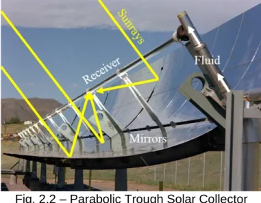
(34) Table 2.1 – Continuation Parabolic Trough Solar Tower. Linear Fresnel. Parabolic Dish. Storage system. Indirect two-tank molten salt at 380°C (ΔT=100K). Direct twotank molten salt at 550°C (ΔT=300K). Short-term pressurized steam storage (<10 min). No storage for Stirling dish, chemical storage under development.. Hybridisation. Yes and direct. Yes. Yes, direct Not planned (steam boiler). Grid stability. Medium to high High (TES or TES) hybridisation). Cycle. Superheated Superheated Rankine steam Rankine cycle steam cycle. (large Medium (back- Low up firing possible) Saturated Stirling Rankine steam cycle. Steam 380 – 540 / 100 conditions (°C / bar). 540 / 100 – 260 / 50 160. n.a.. Maximum <1-2 slope of solar field (%). <2–4. 10 or more. Water requirement (m3/MWh). 3 (wet cooling) 0.3 (dry cooling). 2 – 3 (wet 3 (wet cooling) 0.05 – 0.1 cooling) 0.2 (dry (mirror washing) 0.25 (dry cooling) cooling). Application type. On-grid. On-grid. On-grid. On-grid / off-grid. Suitability for Low to good air cooling. Good. Low. Best. Storage with Commercially molten salt available. Commercially available. Possible, but Possible, not proven not proven. <4. but. TES: Thermal Energy Storage. * upper limit if the solar tower powers a combined cycle turbine. A PTC consists on a reflective surface (mirror) with a linear parabolic shape and a receiver located on the focal line of the cylindrical parabola. Sunrays are reflected by mirrors so the receiver can collect concentrated solar radiation. This radiation is then transformed into heat, and transmitted to a fluid transported through the receiver. Figure 2.2 shows the process to convert solar radiation into heat, as explained before. PTCs operate at low-to-medium temperatures, with the working fluid reaching between 50°C and 400°C. 20.

(35) [3], a range of temperatures where many industrial processes are carried out. Table 2.2 show information about general advantages and disadvantages of PTC technology.. Fig. 2.2 – Parabolic Trough Solar Collector Table 2.2 – Advantages and Disadvantages of PTC technology - Low emissions to the environment during lifespan: According to Burkhardt et al. [4] and Klein and Rubin [5], a Concentrating Solar Power (CSP) plant releases up to 30-70kgCO2eq/MWh, which is lower compared to 400kgCO2eq/MWh reported for a natural gas plant. Advantages. - Lower maintenance and operating (O&M) costs: SEGS plants (California, USA) operates with an estimated cost of USD $ 0.04/kWh [1]. - Long lifespan: PTCs have longer lifespan because they operate at moderate temperatures. - Large land area required: Large areas or land are required to collect enough heat to meet the energy load of the process due to the diffuse nature of solar radiation.. Disadvantages. - High initial investment and medium-long term recovery: The general cost of manufacturing and materials affects the total capital cost, recovery, and levelized cost of energy. - Intermittence of the resource: PTCs use direct solar radiation, so intermittence is a rule as energy cannot be collected at night.. 2.1.2 Components PTCs mainly consists of five principal components: mirrors, a supporting structure, a receiver, working fluid, and a tracking system. Each component accomplishes a specific. 21.

(36) purpose and is made using materials according to its functions and desired properties. These components are explained in detail below. 2.1.2.1 Mirrors Mirrors reflects and concentrates solar radiation into the receiver. They are made of highreflective materials layers (aluminum or silver) with protective-material layers against abrasion or corrosion. The most commonly used materials are silvered glass mirror, anodized sheet aluminum (sometimes coated with a polymer film), aluminized polymers and silvered polymer films. Table 2.3 shows desired properties of materials for mirrors. Optical performance of mirrors can be affected by the surrounding atmosphere, manufacturing, or during normal operation; resulting in a decrement of thermal performance of the collector. Dirt, abrasion, and corrosion can affect the integrity of the mirrors, so it is important to protect them with appropriate coatings. Selecting the appropriate coating based on the desired properties of the reflective surface is mandatory for high thermal performance. Geometrical errors take place in the collector during manufacturing and normal operation, and affect the concentration and consequently, optical efficiency. The most important errors are shape error, slope error, receiver deviation error, specularity error, tracking deviation, and frame deformation. Shape error estimates the eccentricity of the focal line (where the receiver is) due to deviations and misalignments of the mirrors. Slope error measures the deviation of the rays due to slightly ripples presented in the mirror shape. The receiver is not completely aligned to the focal line, so this misalignment is measured by the receiver deviation error. Specularity error refers to the error due to imperfect reflection of mirrors (no-ideal reflective materials). Due to the collector is not always perfectly pointing to the sun, tracking error takes place during operation (See section 2.1.2.5). Another factor that affect the geometry of the collector during operation is normal loading (principally by self-weigth, wind, and torsional loads), which deforms the frame of the collector. These errors are represented in Figure 2.3 (the deviations are exaggerated to illustrate the origin of error).. Fig. 2.3 – Geometrical errors in mirrors 22.

(37) Table 2.3 - Types of mirrors and their properties [7-13] Typical Cost hemispherical ($/m2) reflectance [14]. Type. Description. Up to 0.96. 20 – 30. Silvered glass mirrors. A cooper substrate (replaced by a waterinsoluble precipitate layer in recent years) protected by paint coatings in the back, with a silvered-based coating and a hightransmittance low-reflective glass as cover (superstrate, usually a low-iron glass).. - High resistance to corrosion. - Commercially deployed. - Heavy and fragile.. Polished aluminum sheet with an aluminum-based reflective layer and oxide-enhancing layer.. Up to 0.9. < 20. - Lightweight and flexible. - Low cost. - High variability of durability. - More applicable for lowenthalpy concentrators. - Low durability in polluted locations.. Silvered-reflective layer coated with flexible polymer and a very thin UVscreening film superstrate.. 0.9 – 0.95. 20 – 30. - Under development - Less expensive. High reflectance and lightweight. - Higher flexibility. - Long term performance needs to be proven.. Aluminized reflectors. Silvered polymer reflectors. 23. Properties.

(38) 2.1.2.2 Supporting structure The main function of the structure is to provide stability and rigidity, fixing the receiver and mirrors principally. It is made by structural materials, such as aluminum or steel. The structure can by divided into 3 main sections: -. -. Main support: It serves as anchorage of the collector to the ground. Structurally, the main support must withstand wind loads due to the aperture of the collector being exposed to the wind [15]. Frameworks: Provides rigidity to the mirror in order to maintain its cylindrical parabolic shape. Brackets: Fix the receiver at the focal line of the parabola.. A correct design of frameworks prevents misalignments during operation. The most important mechanical effects to avoid are bending and torsion of the framework, which are principally produced by self-weight and wind forces. Giannuzzi et al. [15] proposed structural design criteria for parabolic trough solar collectors, presenting a methodology to calculate loads for structural designs based on European codes. Common framework designs for PTCs used in CSP plants around the world are the torque box, toque tube, and struts. 2.1.2.3 Receiver The principal function of the receiver is to absorb as much of the reflected solar radiation and to transfer this energy to the Heat Transfer Fluid (HTF) as heat. Receivers are made by a metal pipe coated with a selective material and covered with a glass. The cover glass minimizes heat losses on the pipe and protects it from degradation. A vacuum is applied in the annular region between the glass and the pipe to diminish heat losses and the receiver is sealed to prevent vacuum losses. Figure 2.4 shows the elements of a typical evacuated solar receiver for PTCs.. Fig. 2.4 – PTC solar receiver The ideal material for a pipe receiver should have high resistance to corrosion, low thermal expansion, and high thermal conductivity. The most commonly used materials are stainless steels. Stainless steels have low thermal conductivity, a high resistance to. 24.

(39) corrosion, and they are malleable (so fabrication of tubes is easy). The cover glass is made of a material with high transmittance, low reflectance, and low refractive index. It should transmit the highest possible amount of the incident radiation reflected from the mirrors. Anti-reflective coatings (ARCs) are applied to the external surface of the cover glass to enhance its transmittance. They create a transition on the refractive index from air to the cover [16]. The most commonly used types of glass in solar applications are silica and low-iron glasses (for example, borosilicate is extensively employed in solar applications) [17]. The selective coatings (SCs) absorb as much solar radiation as possible and transmit it to the pipe receiver. They are applied to the external surface of the pipe to increase heat flux absorption. The selective coating should have high shortwave absorptance, low long-wave emittance, good surface adhesion, and chemical stability in the working temperature range of collectors. Table 2.4 shows some prefabricated receivers and their characteristics. 2.1.2.4 Heat transfer Fluid The HTF (also called “working fluid”) is a substance that captures heat coming from the receiver and use it as resource of energy in the process. This fluid should have high thermal capacity and thermal conductivity, low thermal expansion, low viscosity, minimal corrosive activity, low toxicity and thermal and chemical stability throughout its operating temperature range. Properties, advantages, and disadvantages of HTFs used in PTC are shown in Table 2.5. Water and steam are commonly used in low-to-medium enthalpy process, including steam generation. Thermal oils are most used in solar power generation plants, along with a heat exchanger to generate steam for use in a Rankine cycle. Pressurized air is commonly used for drying and heating in buildings using Flat Plate Collectors, but it has been studied as an option for using in PTCs [18]. In fact, some studies suggest good performance in power plants with solar-assisted gas turbines [19-22]. Recently, the use molten salts and ionic liquids with good heat transfer capabilities have been reported in the literature. However, both molten salts and ionic liquids should overcome some challenges such as cost and operational aspects. Nanofluids have been developed for solar energy applications during recent years. A nanofluid is a fluid containing suspended solid nanometer-sized particles called nanoparticles, which increase the heat capacity and thermal conductivity of the mixture. These particles are commonly metals (in natural form or oxides). In the literature, there are some studies on nanofluids with applications in concentrated solar technology. 2.1.2.5 Solar tracking system Main function of solar tracking system is to align the collector with the sun to maximize collector performance by one-axis rotation. Solar trackers can be classified as either passive and active. Passive trackers use the thermosiphon effect to align the collector, whereas active trackers use electronic signal conversion. Passive trackers are not commonly used in PTCs because they could be highly misaligned by wind during operation.. 25.

(40) Table 2.4 - Characteristics of some receivers available in market [23-29] Manufacturer Country. Archimede Solar Energy Italy. Model. HCEMS11. Metal Receiver Length (m) Diam. (mm) Material. 4.06 4.06 70 70 Stainless Steel. HCEOI12. Cover Glass Length (m) 3.9 3.9 Diam (mm) 125 125 Thickness 3 3 (mm) Material Borosilicate (AR coated) Transmittance 0.966 0.966 Selective Coating Absorptance 0.95 0.96 Emittance (@ 0.073 0.085 400°C) Other characteristics Max. operating 30 barg, 37 barg, conditions 580°C 400°C. Siemens (a) Germany. Rioglass Spain UVAC 70- UVAC 7G 90-7G. Sunda China PTR 70- SEIDO 4G 6-1. SEIDO 6-2. SEIDO 6-3. HCESHS12. UVAC 2010. 4.06 70. 4.06 70. 4.06 70. 4.06 88.9. 4.06 70. 2 38. 2 63.5. 4.06 70. 3.9 125. NS 115. NS 115. NS 135. NS 125. NS 102. NS 102. NS 115. 3. NS. 3. 3. 2.5. NS. NS. NS. 0.966. 0.964. 0.967. 0.964. 0.97. 0.95. 0.95. 0.95. 0.95. 0.96. 0.962. 0.962. 0.94. 0.94. 0.94. 0.94. 0.073. 0.09. 0.095. 0.095. 0.095. 0.12. 0.12. 0.12. 104 barg, NS 550°C. Lifetime (yr) 25 25 25 Annulus Pressure < 10-4 < 10-4 < 10-4 (mbar) NS = Not specified (a) Rioglass bought Siemens CSP assets [25]. 40 barg, 40 barg, 41 barg, 15 barg, 30 barg, 40 barg, 350°C 350°C 350°C 300°C 390°C 450°C. 25. 25. 25. 25. NS. NS. NS. < 10-4. < 10-4. < 10-4. < 10-4. NS. NS. NS. 26.

(41) Table 2.5 - Heat transfer fluids used on PTC fields [30-41] Fluid. Water. Working temperature (ºC). Up to 100. General properties. Advantages. Odorless, relative low viscosity, nontoxic.. - No environmental risks (pollution or fire). - Low operational pressures. - Simple plant design.. Disadvantages - Only for low enthalpy applications. - Requires water treatment. - Environmental risks (toxicity).. Glycols. -50 - 300. High heat transfer properties (with combined with water), low viscosity, toxic (depending on the preparation).. - Anti-freezing properties (with the proper concentration).. - Used only in low enthalpy applications (when mixed with water). - Degradation with long-term operation.. Steam. Up to 500. High pressure and temperature applications.. - Higher working temperature.. - Evaporation (two-phase flow, heat losses in flashing).. - Secondary HTF no needed.. - Higher operational pressures.. - No environmental risks (pollution or fire).. - Requires water treatment.. - Easier plant design.. - More complex solar field control. - Lack of suitable TES system.. - Higher steam temperature. Pressurized air. Up to 500. Low cost because of its abundance from atmosphere, low viscosity, low energy density, need to be dehumidified.. 27. - Thermal storage enhancement. - No environmental risks (pollution or fire).. - Poor heat transfer in the receiver. - More complex solar field control. - Higher operational pressures..