TítuloFluid flow simulation by Lagrangian particle methods

Texto completo

(1)European Congress on Computational Methods in Applied Sciences and Engineering ECCOMAS 2004 P. Neittaanmäki, T. Rossi, S. Korotov, E. Oñate, J. Périaux, and D. Knörzer (eds.) Jyväskylä, 24–28 July 2004. FLUID FLOW SIMULATION BY LAGRANGIAN PARTICLE METHODS L.Cueto-Felgueroso, I.Colominas, G.Mosqueira, F.Navarrina, M.Casteleiro? ? Group of Numerical Methods in Engineering, GMNI Dept. of Applied Mathematics, Civil Engineering School Universidad de La Coruña Campus de Elviña, 15192 La Coruña, SPAIN e-mail: cueto@iccp.udc.es, web page: http://caminos.udc.es/gmni/. Key words: Computational Fluid Dynamics, Particle Methods, SPH, Free Surface Flows, Galerkin method. Abstract. In this paper we present a Galerkin based SPH formulation with moving least squares meshless approximation, applied to free surface flows. The Galerkin scheme provides a clear framework to analyze several procedures widely used in the classical SPH literature, suggesting that some of them should be reformulated in order to develop consistent algorithms. The performance of the methodology proposed is tested through various dynamic simulations, demonstrating the attractive ability of particle methods to handle severe distortions and complex phenomena.. 1.

(2) L. Cueto-Felgueroso, I. Colominas, G. Mosqueira, F. Navarrina, M. Casteleiro. 1. INTRODUCTION. The endeavour to solve the continuum equations in a particle (as opposed to cell or element) framework, i.e. simply using the information stored at certain nodes or particles without reference to any underlying mesh, has given rise to a very active area of research: the class of so-called meshless, meshfree or particle methods. If this particle approach is to be used in combination with classical discretization procedures (e.g. the weighted residuals method), then a spatial approximation is required (some kind of “shape functions”, as in the finite element method). Such an interpolation scheme should accurately reproduce or reconstruct a certain function and its succesive derivatives using the nodal values. Furthermore, and in order to achieve computationally efficient algorithms, the interpolation should have a local character, i.e. only a few “neighbour” nodes are considered in the reconstruction process. The origin of modern meshless methods could be dated back to the 70’s with the pioneering works in generalized finite differences and vortex particle methods [1],[2]. However, the highest influence upon the present trends is commonly attributed to early Smoothed Particle Hydrodynamics (SPH) formulations [3],[4],[5], where a lagrangian particle tracking is used to describe the motion of a fluid. Although this general feature is shared with vortex particle methods, SPH includes a spatial approximation framework (some kind of “meshfree shape functions”), developed using the concept of kernel estimate. The Smoothed Particle Hydrodynamics (SPH) method was developed to simulate fluid dynamics in astrophysics [3],[4]. The extension to solid mechanics was introduced by Libersky, Petschek et al. [6] and Randles [7]. Johnson and Beissel proposed a Normalized Smoothing Function (NSF) algorithm [8] and other corrected SPH methods have been developed by Bonet et al. [9],[10] and Chen et al. [11]. More recently, Dilts has introduced Moving Least Squares (MLS) shape functions into SPH computations [12]. Early SPH formulations included both a new approximation scheme and certain characteristic discrete equations (the so-called SPH equations), which may look quite “esoteric” for those researchers with some experience in methods with a higher degree of formalism such as finite elements. The formulation described in this paper follows a different approach, and the discrete equations are obtained using a Galerkin weighted residuals scheme. This derivation may result somewhat disconcerting for those accustomed to the classical SPH equations. However, we believe that Galerkin formulations provide a strong framework to develop consistent algorithms. The outline of the paper is as follows. We begin with a brief review of standard SPH and moving least squares approximations. After introducing the model equations, their discrete counterpart is obtained using a Galerkin formulation. Finally, the methodology is applied to the simulation of fluid dynamics and free surface flows.. 2.

(3) L. Cueto-Felgueroso, I. Colominas, G. Mosqueira, F. Navarrina, M. Casteleiro. 2. MOVING LEAST-SQUARES APPROXIMATION. x) defined in a bounded, or unbounded, domain Ω. The Let us consider a function u(x x), at a given point x, through a basic idea of the MLS approach is to approximate u(x x) in a neighbourhood of x as: polynomial least-squares fitting of u(x x) ≈ ub(x x) = u(x. ¯. m X. ¯. x)αi (zz )¯¯ x)α α(zz )¯¯ pi (x = pT (x z =x z =x i=1. (1). ¯. x) is an m-dimensional polynomial basis and α (zz )¯¯ where pT (x is a set of parameters to z =x be determined, such that they minimize the following error functional: Z. ¯ α(zz )¯¯ J(α. z =x ¯. )=. ¯. ¯. h. i2. ¯ α(zz )¯¯ W (zz − y , h)¯ u(yy ) − pT (yy )α dΩx z = x z =x y ∈Ωx. (2). being W (zz − y , h)¯¯ a symmetric kernel with compact support (denoted by Ωx ), frez =x quently chosen among the kernels used in standard SPH. The parameter h is called smoothing length, and measures the size of Ωx . The stationary conditions of J with respect to α lead to Z. ¯. ¯. x)α α(zz )¯¯ p(yy )W (zz − y , h)¯¯ u(yy )dΩx = M (x z = x z =x y ∈Ωx. (3). x) is where the moment matrix M (x Z. x) = M (x. ¯. ¯ p(yy )W (zz − y , h)¯ pT (yy )dΩx z =x y ∈Ωx. (4). In numerical computations, the global domain Ω is discretized by a set of n particles. We can then evaluate the integrals in (3) and (4) using those particles inside Ωx as quadrature points (nodal integration) to obtain, after rearranging, ¯. ¯ x)u uΩx x)P P Ωx W V (x (5) α (zz )¯ = M −1 (x z =x where the vector uΩx contains certain nodal parameters of those particles in Ωx , the x) = PΩx WV (x x)PTΩx , and matrices PΩx and WV (x x) can be discrete version of M is M(x obtained as: ³. x1 ) p(x x2 ) PΩx = p(x. ···. x) = diag {Wi (x x − xi )Vi } , WV (x. ´. xnx ) p(x. i = 1, . . . , nx. (6) (7). Complete details can be found in [13]. In the above equations, nx denotes the total number of particles within the neighbourhood of point x and Vi and xi are, respectively, the tributary volume (used as quadrature weight) and coordinates associated to particle i. Note that the tributary volumes of neighbouring particles are included in matrix 3.

(4) L. Cueto-Felgueroso, I. Colominas, G. Mosqueira, F. Navarrina, M. Casteleiro. WV , obtaining an MLS version of the Reproducing Kernel Particle Method (the so-called MLSRKPM) [14]. Otherwise, we can use W instead of WV , x) = diag {Wi (x x − xi )} , W(x. i = 1, . . . , nx. (8). which corresponds to the classical MLS approximation (in the nodal integration of the functional (2), the same quadrature weight is associated to all particles). Introducing (5) in (1) the interpolation structure can be identified as: x) = pT (x x)M−1 (x x)P x)u uΩx = N T (x x)u uΩx ub(x P Ωx W V (x. (9). And, therefore, the MLS shape functions can be written as: x) = pT (x x)M−1 (x x)P P Ωx W V (x x) N T (x 3. (10). A LAGRANGIAN PARTICLE SCHEME FOR FREE SURFACE FLOWS. 3.1. Continuum equations. Let us assume a compressible, newtonian fluid, thus behaving as if it was governed by the following set of equations: (a) Continuity equation: dρ = −ρ div(vv ) dt. (11). d· denotes the material time derivative and div(vv ) is computed in the current where dt configuration in terms of the velocity gradient tensor l div(vv ) = tr(ll ),. l=. x, t) ∂vv (x = ∇x v x ∂x. (12). (b) Momentum equation: dvv = ∇x · σ + b (13) dt where ρ is the density and the stresses are related to the Cauchy stress tensor σ ρ. d0 σ = −pII + 2µd. (14). in terms of the pressure p, the viscosity µ and the deviatoric part (dd0 ) of the rate of deformation tensor d, given by. 4.

(5) L. Cueto-Felgueroso, I. Colominas, G. Mosqueira, F. Navarrina, M. Casteleiro. 1 1 d)II , ∇x v + ∇x v T ) d0 = d − tr(d d = (∇ 3 2 We use an equation of state of the form [16]: ·µ. p=κ. ρ ρ0. ¶γ. (15). ¸. −1. (16). where typically γ = 7 and κ is chosen such that the fluid is nearly incompressible. In gravity flows the initial particle densities are adjusted to obtain the correct hydrostatic pressure computed as (16) [16]: µ. ρ0 g(H − z) ρ = ρ0 1 + κ where H is the total depth and g = 9.81 m/s2 .. ¶1/γ. (17). (c) Angular Momentum Conservation: We consider neither mass distributions of polar momenta nor magnetizable media. (d) Energy equation: Conservation of energy may also be considered in processes involving heat transfer or other related phenomena: dU = σ : d − div(qq ) + ρQ (18) dt where U is the internal energy per unit mass, q is the energy flux, Q a thermal source (energy per unit time and mass) and d is the rate of deformation tensor ρ. 3.2. Discrete equations. The meshless discrete equations can be derived using a weighted residuals formulation. The discrete counterpart of the Galerkin weak form is almost equivalent to that obtained from kernel estimates [17] such as classical SPH formulations. Furthermore, such an equivalence indicates that SPH can be studied in the context of Galerkin methods. The global weak (integral) form of the spatial momentum equation can be written as: Z Z Z dvv (19) ρ · δvv dΩ = − σ : δll dΩ + b · δvv dΩ + σ n · δvv dΓ Ω Ω Γ Ω dt being Ω the problem domain, Γ its boundary and n the outward pointing unit normal to the boundary. If δvv and v are approximated by certain test and trial functions δvb and vb, Z. Z Ω. ρ. Z Z Z dvb · δvb dΩ = − σb : δbl dΩ + b · δvb dΩ + σb n · δvb dΓ dt Ω Ω Γ. 5. (20).

(6) L. Cueto-Felgueroso, I. Colominas, G. Mosqueira, F. Navarrina, M. Casteleiro. The spatially discretized equations are obtained after introducing meshless test and trial functions and their gradients in (20) as x) = δvb(x. n X. x), δvv i Ni∗ (x. n X. x) = ∇δvb(x. i=1. x) = vb(x. n X. x) δvv i ⊗ ∇x Ni∗ (x. (21). i=1. x), v j Nj (x. n X. x) = ∇vb(x. j=1. x) v j ⊗ ∇x Nj (x. (22). j=1. to yield, n X i=1. δvv i ·. ½X n Z j=1 Ω. x)Nj (x x) ρNi∗ (x Z. −. Z dvv j x)dΩ− dΩ + σb ∇x Ni∗ (x dt Ω ¾. Z. Ω. x)bb Ni∗ (x. dΩ −. Γ. x)σb n Ni∗ (x. dΓ = 0. (23). Thus, for each particle i the following identity must hold: n Z X j=1 Ω. dvv j x)Nj (x x) dΩ ρNi∗ (x dt. Z. Z. =−. Ω. x)dΩ + σb ∇x Ni∗ (x. Ω. Z. x)bb Ni∗ (x. dΩ +. Γ. x)σb n dΓ (24) Ni∗ (x. In this paper we follow a Bubnov Galerkin approach and, therefore, Nj∗ = Nj . For convenience, we can write (24) in a compact form: M a = F int + F ext. (25). where the mass matrix M = {mij }, internal forces F int = {ff int i } and external forces F ext = {ff ext } are respectively defined by: i Z. mij =. Ω. x)Nj (x x)dΩ ρNi∗ (x. (26). Z. f int =− i. Ω. x)dΩ σb ∇x Ni∗ (x Z. Z. f ext = i. Ω. (27). x)bb dΩ + Ni∗ (x. Γ. x)σb n dΓ Ni∗ (x. (28). If expression (11) is used for mass conservation, its Galerkin weak form is equivalent to a point collocation scheme and, thus, the continuity equation must be enforced at each particle i, n X dρi xi ) = −ρi div(vv )i = −ρi v j · ∇x Nj (x dt j=1. 6. (29).

(7) L. Cueto-Felgueroso, I. Colominas, G. Mosqueira, F. Navarrina, M. Casteleiro. where expression (22) for ∇vbi has been used. Nodal integration has been used, at least implicitly, in most SPH formulations, and lies, indeed, in the basis of its early formulation. Obviously, this is the cheapest option and the resulting scheme is truly meshless (no background mesh is needed). The particles are used as quadrature points and the corresponding integration weights are their tributary volumes. Recalling the weak form derived in the previous section, the discrete eulerian momentum equation can be written as: M a = F int + F ext. (30). where mij =. n X. xk )Nj (x xk )Vk ρk Ni∗ (x. (31). k=1. f int =− i. n X. xk )Vk σb k ∇x Ni∗ (x. (32). k=1. f ext = i. n X. xk )bbk Vk + Ni∗ (x. n X. xk )σb k nAk Ni∗ (x. (33). k=1. k=1. In the above, Vk represents the tributary volume associated to particle k. Usual techniques to determine such volumes vary from simple domain partitions to Voronoi diagrams. In the most frequent approach in SPH simulations, the particles are set up with certain initial densities, volumes and, therefore, masses. These physical masses {Mk } remain constant during the simulation and densities are field variables updated using the continuity equak tion. Thus, particle volumes are obtained for each time step as Vk = M . Note that, in ρk our formulation, the real or physical particle masses Mk are different, in general, from the numerical masses mij given by (31), and derived in the Galerkin scheme. In practice, it is more efficient to use a lumped mass matrix with the real particle masses as numerical masses. We use explicit time integration to update the field variables. One of the most widely used algorithms is the leap-frog scheme, involving the following sequence of updates: • Compute velocities at step k + 12 : k+ 21. vi. k− 12. = vi. aki + 0.5(∆tk + ∆tk+1 )a. (34). • Update densities and positions: 1. ρk+1 = ρki + ∆tk+1 Di (vv k+ 2 ) i k+ 12. = xki + ∆tk+1vbi xk+1 i. 7. (35) (36).

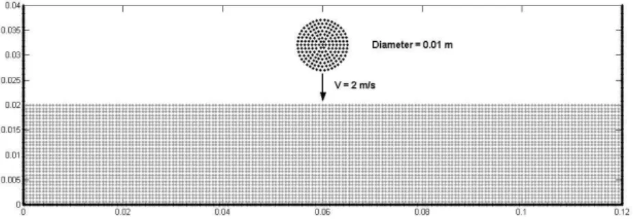
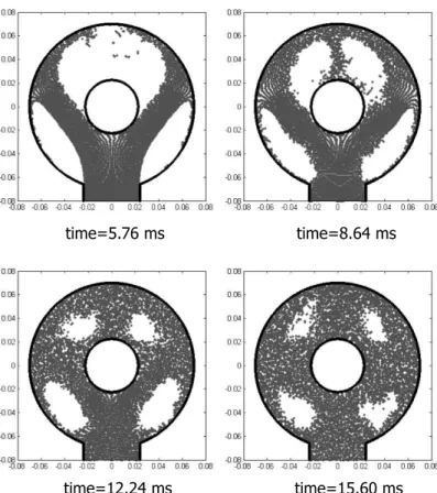
(8) L. Cueto-Felgueroso, I. Colominas, G. Mosqueira, F. Navarrina, M. Casteleiro dv k In the above expressions, aki = dti is the acceleration nodal parameter of particle i 1 (computed by using the momentum equation with variables at step k) and Di (vv k+ 2 ) is k+ 1. i the density rate dρ , computed with positions at step k and intermediate velocities v i 2 . dt With vbi we denote the interpolated nodal velocities. The time step is limited by the Courant-Friedrichs-Lewy (CFL) stability condition:. ∆t = CF L. hmin max(ci + kvv i k). (37). where CF L is the Courant number (0 ≤ CF L ≤ 1) and ci is the wave celerity at point i, q. ci =. γκ/ρi. (38). being γ and κ the same material properties as in (16). More detailed information about the formulation proposed can be found in [18]. 4. NUMERICAL EXAMPLES. In the first example a circular drop of water falls vertically at 2 m/s on a mass of water initially at rest (Figures 1 and 2). This example demonstrates the good performance of the method in the absence of boundary distortions (Figure 3). The fluid density and viscosity are ρ0 = 1000 kg/m3 and µ = 0.5 kg m−1 s−1 , respectively. The total number of particles is 5539.. Figure 1: Fluid-Fluid Impact: Scheme of the initial configuration.. The second simulation corresponds to the filling of a circular mould with core (Figure 4). The velocity of the jet at the gate is 18 m/s and the viscosity is µ = 0.01 kg m−1 s−1 . The bulk modulus κ was chosen such that the wave celerity is 1000 m/s and the total number of particles is 14314. Several instants of the simulation are shown in Figure 5, with times referred to the impact between the jet and the core. The overall shape of the two jets passing the core looks quite satisfactory and agree with previous results [19]. In spite of using a consistent formulation of boundary forces, we have found excessive distortion near the boundaries, compared with the flow away from their influence (see 8.

(9) L. Cueto-Felgueroso, I. Colominas, G. Mosqueira, F. Navarrina, M. Casteleiro. time=0.0018 s. time=0.0099 s. time=0.0297 s. time=0.0477 s. time=0.0657 s. time=0.0837 s. time=0.1017 s. time=0.1197 s. time=0.1377 s. time=0.1557 s. Figure 2: Fluid-Fluid Impact: Simulation at various stages.. Figure 6). This effect could be caused by the “particle based” boundary approach. We expect to develop better algorithms in the future. Figure 7 shows a comparison between the solution computed and the experiments carried out by Schmid and Klein [20].. 9.

(10) L. Cueto-Felgueroso, I. Colominas, G. Mosqueira, F. Navarrina, M. Casteleiro. Figure 3: Fluid-Fluid Impact: Simulation at t = 0.0396 s (detail).. Figure 4: Mould filling: Dimensions of the mould.. 5. CONCLUSIONS. In this study we explored the application to free surface flows of a Galerkin based SPH formulation with moving least squares meshless approximation. The Galerkin scheme provides a clear framework to analyze several procedures widely used in the classical SPH literature, suggesting that some of them should be reformulated in order to develop consistent algorithms. The performance of the methodology proposed was tested through various dynamic simulations, demonstrating the attractive ability of particle methods to handle severe distortions and complex phenomena.. 10.

(11) L. Cueto-Felgueroso, I. Colominas, G. Mosqueira, F. Navarrina, M. Casteleiro. time=5.76 ms. time=8.64 ms. time=12.24 ms. time=15.60 ms. Figure 5: Mould filling: Simulation at various stages.. Figure 6: Mould filling: Simulation at t = 5.76 ms.. 11.

(12) L. Cueto-Felgueroso, I. Colominas, G. Mosqueira, F. Navarrina, M. Casteleiro. Figure 7: Mould filling: Experimental (left) and numerical (right) results.. 6. ACKNOWLEDGEMENTS. This work has been partially supported by the SGPICT of the “Ministerio de Ciencia y Tecnologı́a” of the Spanish Government (Grant DPI# 2001-0556), the “Xunta de Galicia” (Grants # PGDIT01PXI11802PR and PGIDIT03PXIC118002PN) and the University of La Coruña. Mr. Cueto-Felgueroso gratefully acknowledges the support received from “Fundación de la Ingenierı́a Civil de Galicia” and “Colegio de Ingenieros de Caminos, Canales y Puertos”. This paper was written while Mr. Cueto-Felgueroso was visiting the University of Wales Swansea during the first semester of 2004. The support received from “Caixanova” and the kind hospitality offered by Prof. Javier Bonet and his research group are gratefully acknowledged.. 12.

(13) L. Cueto-Felgueroso, I. Colominas, G. Mosqueira, F. Navarrina, M. Casteleiro. REFERENCES [1] T. Belytschko, Y. Krongauz, D. Organ, M. Fleming, P. Krysl, Meshless methods: An overview and recent developments. Computer Methods in Applied Mechanics and Engineering, 139, 3–47 (1996). [2] A.J. Chorin. Numerical study of slightly viscous flow. Journal of Fluid Mechanics, 57 (1973). [3] L.B. Lucy, A numerical approach to the testing of the fission hypothesis. Astronomical Journal, 82, 1013 (1977). [4] R.A. Gingold, J.J. Monaghan, Smoothed Particle Hydrodynamics: theory and application to non-spherical stars. Monthly Notices of the Royal Astronomical Society, 181, 378 (1977). [5] J.J. Monaghan, An introduction to SPH. Computer Physics Communications, 48, 89–96 (1988). [6] L.D. Libersky, A.G. Petschek, T.C. Carney, J.R. Hipp, F.A. Allahdadi, High strain Lagrangian hydrodynamics. Journal of Computational Physics, 109, 67–75 (1993). [7] P.W. Randles, L.D. Libersky, Smoothed Particle Hydrodynamics: Some recent improvements and applications. Computer Methods in Applied Mechanics and Engineering, 139, 375–408 (1996). [8] G.R. Johnson, S.R. Beissel, Normalized Smoothing Functions for SPH impact computations. International Journal for Numerical Methods in Engineering, 39, 2725–2741 (1996). [9] J. Bonet, T-S.L. Lok, Variational and momentum preserving aspects of smooth particle hydrodynamics (SPH) formulations. Computer Methods in Applied Mechanics and Engineering, 180, 97–115 (1999). [10] J. Bonet, S. Kulasegaram, Correction and stabilization of smoothed particle hydrodynamics methods with applications in metal forming simulations. International Journal for Numerical Methods in Engineering, 47, 1189–1214 (2000). [11] J.K. Chen, J.E. Beraun, A generalized smoothed particle hydrodynamics method for nonlinear dynamic problems. Computer Methods in Applied Mechanics and Engineering, 190, 225–239 (2000). [12] G.A. Dilts, Moving-Least-Squares-Particle Hydrodynamics. International Journal for Numerical Methods in Engineering, Part I 44, 1115-1155 (1999), Part II 48, 1503 (2000). 13.

(14) L. Cueto-Felgueroso, I. Colominas, G. Mosqueira, F. Navarrina, M. Casteleiro. [13] W.K. Liu, S. Li, T. Belytschko, Moving least-square reproducing kernel methods: (I) Methodology and Convergence. Computer Methods in Applied Mechanics and Engineering, 143, 113–154 (1997). [14] L. Cueto-Felgueroso, Una visión general de los métodos numéricos sin malla: formulación y aplicaciones. Proyecto Técnico, Universidad de La Coruña, (2002). [15] J.P. Morris, An Overview of the Method of Smoothed Particle Hydrodynamics. Universitat Kaiserslautern. Internal Report (1995). [16] J.J. Monaghan, Simulating Free Surface flows with SPH. Journal of Computational Physics, 110, 399–406 (1994). [17] T. Belytschko, Y. Guo, W.K. Liu, S.P. Xiao. A unified stability analysis of meshless particle methods. International Journal for Numerical Methods in Engineering, 48, 1359–1400 (2000). [18] L. Cueto-Felgueroso, I. Colominas, G. Mosqueira, F. Navarrina, M. Casteleiro, On the Galerkin formulation of the Smoothed Particle Hydrodynamics method. International Journal for Numerical Methods in Engineering, [en prensa] (2003). [19] P. Cleary, J. Ha, V. Alguine, T. Nguyen, Flow modelling in casting processes. Applied Mathematics and Modelling, 26, 171–190 (2002). [20] M. Schmid, F. Klein. Fluid flow in die cavities - experimental and numerical simulation, NADCA 18. International Die Casting Congress and Exposition. Indianapolis (1995).. 14.

(15)