A Cost Function for Internet With QoS Parameters Única

Texto completo

(1)Instituto Tecnológico y de .Estudios Superiores de Monterrey Campus Monterrey Di v is ión de Graduados en ComputaciOn, In Información y Comunicacjones. Programa de Graduados en Cornputación, In form ación y Comunicaciones. A cost function for Internet with QoS parameters. THESIS Presented as part al iu~ lli ment of the requirements for the degree of Master of’ Science in Electronic. Engineering. Major in Telecommunications. Man riclo de Medina Agtiilera. August 1999.

(2) Instituto Tecnológico y de Estudios Superiores de Monterrey Campus Monterrey Division de Graduados en Computación, Inforrnación y Comunicaciones Programa de Graduados en Computación, Inforrnación y Cornunicaciones. A cost function for Internet with QoS parameters. THESIS. Presented as a partial fulfillment of the requirements. for the degree of. Master of Science in Electronic Enginnering Major in Telecommunications. Mauricio de Medina Aguitera August 1999.

(3) Aknowledgments. I want to thank Instituto Tecnologico y de Estudios Superiores de Monterrey (ITESM), for the opportunity to perform my studies of Master Deegre.. I am grateful to my thesis advisor, Cesar Vargas Rosales, Ph. D.; this work could not have been possible without his interest and collaboration.. I also want to thank Artemio Aguilar, M. Sc., and Leoncio Pardo, M. Sc., for their valuable comments.. Thanks to all my fellow students at CET.. Thanks to my entire family for their support and love..

(4) Abstract Nowadays the number ofusers in the Internet is growing in an exponentially way and there arc several applications that the Internet offers and these require to be handled in different ways to run efficiently and improve the use of the network resources. We proposed a revenue function that allows the service provider to know their maximum revenue based on some parameters such as. —. the average number of packets, the. average delay, the arrival rates, the capacity in the network links- and associate it with costs. In order to obtain the revenue function, we established a network topology with two different classes of traffic, the delay permissible for each one and the capacity in the links of the network. We used the Broyden-Fletcher-Goldfarb-Shanno (BFGS) method to maximize the revenue function. We compare the optimized values versus non optimized values to observe their differences and how they rebound in the network performance and it is possible to control the network based on the prices..

(5) Table of Contents Chapter 1 Introduction. 1. 1.1 Objective. 2. 1.2 Justification. 2. 1.3 Contribution. 2. 1.4 Organization. 3. Chapter 2 Pricing the Internet. 4. 2.1 Internet Architecture and Mechanisms. 4. 2.2 Internet Technology. 5. 2.3 The current Internet pricing model. 6. 2.4 Effects on and Inputs for Pricing schemes. 8. 2.5 Variability of prices. 9. Chapter 3 Model Description. 12. 3.1 Background. 12. 3.2 Types of application. 13. 3.3 Description of the network. 14. 3.4 Performance measures. 15. 3.5 Revenue Function. 18. Chapter 4 Numerical Results. 21. 4.1 Network Model. 21. 4.2 Optimization method. 24. 4.3 Basic Scenario. 25. 4.4 Quality ofService variation. 33. Chapter 5 Conclusions and Future work. 37. Bibliography. 39.

(6) List of Figures Figure 1. Two equal capacity transmission lines in tandem. 13. Figure 2 Connection between nodes. 15. Figure 3. Relationship between 2,~and 1u~. 17. Figure 4. Network simulated with his respective paths. 22. Figure 5. Revenue as a function of external rate for optimized and non optimized cases. 26. Figure 6. Average number of packets in link 1 for optimized and non optimized cases. 26. Figure 7. Average number of packets for class 1 for optimized and non optimized cases. 27. Figure 8. Average delay in link 1 for optimized and non optimized cases. 28. Figure 9. Average delay in class 1 in link 1 for optimized and non optimized cases. 28. Figure 10. Revenue as a function of QoS for each class. 34. Figure 11. Average delay in the network for each class. 35. Figure 12. Carried traffic in the network as QoS per class is varied. 36. List of equations Equation 1. Total arrival rate per link. 15. Equation 2 Average number of packets per link and class. 16. Equation 3. Average number of packets per link. 16. Equation 4. Average number ofpackets in the network per link and class. 17. Equation 5. Average delay per packet per link and class. 17. Equation 6. Average delay per packet per link. 18. Equation 7. Average delay per packet in the system. 18. Equation 8 Cost function. 19. Equation 9. Revenue constraints. 24.

(7) List of Tables Table 1. Values of arrival rates per class per time unit. 24. Table 2. Exceeding the capacity in the link 1 class 1. 29. Table 3. Rebounds in the relationship QoS. 29. —. Delay. Table 4. Optimized arrival rates by varying c~1in link 1. 30. Table 5. Optimized arrival rates by varying wd in link 1. 30. Table 6. Optimized arrival rates by varying c~in link 4. 31. Table 7. Optimized arrival rates by varying w~in link 4. 32. Table 8. Average delay per class k in the connection varying w~. 32. Table 9. Average delay per class k in the connection varying c~,. 33.

(8) Chapter 1 Introduction Networks such as Internet are actually providing a wide variety of services, which are consuming widely differing amounts ofresources. It is correct that the technology is increasing, but so is the demand. Different kinds of traffic require different treatment on the network. The usage prices are not a good way to recover the cost of providing network capacity. Since the network costs are primarily the fixed cost of capacity, it makes more sense to charge users a fixed fee depending on the resources of their connection to the net. This is essentially the scheme that is used now. For a pricing system to be “incentive compatible” it is necessary that the use ofhigher quality service incur a higher cost to the user. With the growing demand for multimedia, it is necessary to think about the allocation of multiple service qualities in an integrated network. For example, file transfers tolerate zero errors, but can tolerate substantial delay, on the other hand interactive video can tolerate some packet loss, but requires tight bounds on maximum delay and variation in delay. In this thesis a cost function is proposed and analyzed to observe the behavior of the network under a pricing scheme. Three stages need to be followed in order to provide good pricing schemes that optimize network performance. The first stage consists of defining the traffic classes, the QoS (Quality of Service) parameters to be satisfied as well as an objective function to be optimized which represents network net revenue, the optimization considers flat revenues and costs along the resources, services and routes..

(9) The second stage is to consider the control of the traffic by varying the revenues and costs such that performance is maximized. The third stage is to consider different pricing schemes such as usage based [9], edge pricing [12], etc., and determine a pricing strategy such that dynamically controls network performance in an optimized form.. 1.1 Objective The aim ofthis work is to analyze the behavior ofa network such that its processes give insight the behavior of the Internet by using QoS parameters to give a cost to the user and optimize performance of the network. We propose a cost function for the Internet Service Provider such that he knows the traffic that allows have the greatest profit under some scenarios. We will gain insight on the issue of traffic control through pricing strategies.. 1.2 Justification. Due to the growth of users at Internet and the inefficiency of giving a “good service,” it is becoming important to increase the service and quality given by the network. As well as the revenues keeping prices low. Since different classes of traffic require different treatment from the network and it is necessary to optimize the resources of it, for this reason it is becoming important to have a function that allows the service provider to know the maximum utility.. 1.3 Contribution We have proposed a cost function in relation to the average number of packets, the average delay in the network, the number of links, the arrival and the departure rate in the network, the QoS necessary for different kinds of traffic and we have included a cost per link and per application..

(10) 1.4 Organization The content of this thesis is organized as follow. In Chapter two the concepts about Internet and the current pricing model are presented. In the Chapter three introduces the performance measures, the analytical model and the cost function, also the parameters and assumptions involved in our scenario. Chapter four presents the numerical results comparing a scheme using optimization of the cost function and without optimizing it and varying the variables involved. Finally, in Chapter five we present conclusions and suggest future work to continue with the issue of this thesis.. 3.

(11) Chapter 2 Pricing the Internet In this chapter we explain the characteristics ofthe Internet and we introduce the theoretical aspects ofpricing in networks, we discuss the current pricing scheme and how the pricing can be made.. 2.1 Internet Architecture and Mechanisms The current Internet architecture is designed for point-to-point (or unicast) best-effort communication. Every packet header contains a source address and a destination address. Upon receiving a packet, a switch (or, equivalently, a router) consults its routing table to find, based on the packet’s destination address, the appropriate outgoing link for the packet. The network makes no commitments about when, or even if, packets will be delivered. Sometimes the incoming rate of packets at a switch is greater than the outgoing rate, so queues build up in the switch. These queues cause packet delays and, if the switch runs out of buffer space, packets are discarded. The network does not attempt to schedule use; a source can send packets at any time, and the network switches merely exert their best effort to handle the load, [2]. However, there are efforts currently underway to extend this architecture in two ways. The first is to offer better support for multipoint-to-multipoint communications through the use of multicast. In the current Internet architecture, when a source sends a packet to multiple receivers, the source must replicate the packet and send one to each receiver individually. This results in several copies of the same packet traversing those links common to the delivery paths (i.e., those links that lie on more than one delivery path, where the delivery path is the route taken by the packet from source to receiver).. 4.

(12) Nowadays the efforts extend the Internet’s current service offerings to include a wider variety of qualities ofservice (QoS). Actually the Internet has characteristics there is to take into account. First the overall bandwidth is quite limited which restricts the aggregate traffic load and prevents certain bandwidth-intensive applications from utilizing the Internet. Second, access to the Internet is severely restricted; this is in past because of the limited bandwidth available. Third, the Internet offers a single type of service (TOS); all packets are serviced on a best-effort, first-in-first-out (FIFO) basis. This single TOS severely limits the nature of applications that can be adequately supported. Fourth, there are no usage fees; users are not charged on the basis of how many packets they send, these fees are not based on the volume of traffic sent, [6], and are typically not passed back to individual users. The current single class of best-effort service may not be sufficient to adequately support the requirements of some future video and voice applications. Moreover, offering all applications the same service is not an efficient use of bandwidth; providing several service priority levels and/or drop priority levels, [12]. 2.2 Internet Technology The Internet network uses packet-switching communications technology based on the TCP/IP protocols. While much of the traffic moves across leased lines from Network service providers, packet-switching technology is quite different from the circuitswitching used for voice telephony, where at the moment a telephone user dials a number, a dedicated path is set up between the caller and the called number. This path, with a fixed amount of network resources, is held open; no other caller can use those resources until the call is terminated. Packet-switching network, by contrast, uses ‘statistical multiplexing”, this means that each circuit is shared by many users, and no open connection is maintained for a particular communications session. Data streams are little pieces called “packets”. When a packet is ready, the computer sends it onto the network. When one computer is not sending a packet, the network line is available for packets from other computers. The destination does not need to be aware that a packet has been sent to it.. 5.

(13) The TCP (Transmission Control Protocol) provides how to break up a data stream into packets and reassemble it; the IP (Internet Protocol) provides the necessary information for various computers on the Internet (the routers) to move the packet to the link on the way to its final destination.. The other distinguishing feature of Internet technology is that it is ‘connectionless”. This means that there is no end-to-end setup for a session; each packet is independently routed to its destination. When a packet is ready, the host computer sends it to another computer, known as a router. The router examines the destination address in the header and passes the packet along to another router, chosen by a routefinding algorithm, [I].. 2.3 The current Internet pricing model We know that the Internet transport is already priced, although many users seem unaware of it. Pricing is on the basis of a fixed monthly subscription fee for a connection of a given bandwidth (called flat rate pricing). Most ofthe costs of providing the Internet are more-or-less independent of the network; i.e. most of the costs are fixed costs. If the network is not saturated the incremental cost of sending additional packets is essentially zero. In most cases the incremental usage of that bandwidth is priced at a flat rate of zero, [4]. Given that congestion is likely to be a serious problem in the near future of the Internet, and past proposals for its control unsatisfactory, it is beneficial to consider other pricing schemes that take into account incremental costs and allow some congestion control. Since the bandwidth is scarce, when the backbone or the capacity of the links becomes congested, one user’s packet crowds out another’s, resulting in dropped or delayed transmissions. Allocating scarce resources among competing uses is the central focus of economics. One of the fundamental principles of economics is that prices should reflect costs. In addition the pricing may discourages network usage by customers in times of high network load or congestion due to higher prices and it provides revenue for providers which may be used to extend or renew the current networking infrastructure and capacities.. 6.

(14) As a general rule, users should face the prices that reflect the resource costs that they generate so they can make informed decisions about resource utilization. Some ways to do these are, [5]: The incremental cosis of sending extra packets. The price of sending a packet in an uncongested network should be close to zero; a higher price is socially inefficient since it does not reflect the true incremental costs. But if the network is congested there is more probability of delay and dropped packets so that some packets should be retransmitted. The social costs c/delaying other user ‘s packets when the network is congested. When the network is congested due to large amounts of frames crossing it, this causes a significant delay in all users. The fixed costs ofproviding the network infrastructure. In the case of a computer network like Internet, it is natural to think of paying for the network infrastructure with a flat access fee. Each party who connects to the network pays a flat price for network access distinct from the usage-based fee described earlier. In general, these connection fees will vary, since different people and institutions value connection to the net differently. If the total amount that users are willing to pay exceeds the infrastructure cost, the fees could be assigned in a variety of ways, depending on the market conditions and the network providers’ objectives.. 7.

(15) The incremental costs of connecting to the network.. If network usage never reaches capacity, even at no costs for packets, then clearly there is no need to expand capacity. Usage prices that are based on congestion provide. guidance about when to expand capacity. Consider the model with fixed capacity: Packet prices measure the marginal value of the last admitted packet. If the cost of expanding capacity to accommodate one more packet is less than the marginal value of that packet, then it makes economic sense to expand capacity. The incremental costs of using more links. When the network has its capacity or router full or even is incapable of giving a QoS acceptable it is necessary to follow another path, where in some cases the route taken will be more expensive since the path taken uses more resources because it is using more links or using links dedicated to give another class of service or is full also.. 2.4 Effects on and Inputs for Pricing schemes Any pricing scheme or policy is affected by at least eight factors that encompass the economic, the technological, and the administrative situation, these form the market structure of the network, [11]:. •. cost recovery. •. network demand. •. network load. •. cost of working equipment. •. type of services. •. capacity expansion. •. regulatory environment. 8.

(16) A pricing scheme has to take into account the market in which communication services are offered. It needs to recover costs fully that are based on the provision ofthe network infrastructure and the equipment, its maintenance, its investment for future enhancements and extensions, and its offered type of services. Additionally, special legal restrictions for applying schemes have to be obeyed. Furthermore, a pricing scheme has to follow certain goals to be suitable as a monetary incentive. These economic goals include at least: (1) optimal efficiency to gain maximal welfare, (2) maximize the total utility of all users, (3) maximize the utility ofa specific resource, (4) maximize profit, (5) fairness, and (6) recover costs fully, [8]. Pricing schemes or changes that are designed to recover costs fairly from this diverse population of users and to allocate network resources in an efficient manner require the capability to measure individual user traffic and to present users with prices and charges in a way that encourages efficient network use. One incentive to reduce technical demands is a fair pricing scheme that takes into account the requested service class or QoS per streams.. 2.5 Variability of prices Prices may vary based on a number of different factors. These factors sometimes determine the charging unit, a certain period of time when the price is valid, or administrative issues. They can include different criteria, features or combination of them such as the usage of a particular resource, network access, Quality of Service (QoS) requirements, congestion level of the network. ,. time-of-day, duration,. destination, distance or number of hops to be traversed, requested service class, demand and. supply,. network. providers. and. their. cost. structures,. networking. equipment/technology, tariffing acts, legal issues, per- packet, per-reservation, per flow, per-call, per-connection, per-day, week or month, [11]. The satisfaction that a network user derives from his/her network access depends on the nature of the application being used and the quality of service received from the network (in terms of bandwidth, delay, packet dropped, etc.); the network resources are used most efficiently if they maximize the total user satisfaction of the user community.. 9.

(17) One component of network charges is the attachment fee; this is the fee charged for gaining access to the network and is independent of any actual or potential usage. One minimal requirement is that pricing should encourage the appropriate use of quality of service (Q0S) signals (this means the signals sent by applications to the network requesting a particular quality of service). This is crucial for making the new QoS-rich network designs effective, and would enable them to achieve significant increases in network efficiency. An additional requirement is that pricing should discourage network usage during times of congestion, but not discourage it during relatively uncongested times somewhat vaguely like the telephone companies. Pricing and type of service. Different kinds of traffic require different treatment from the network. E-mail can be delayed without much loss; real-time video needs very rapid service. In order to provide appropriate treatment for different kinds of services, the network needs to know what type of traffic is actually flowing and the traffic required. For this, the routers must be capable of distinguish the type of traffic or the person who generates the data must indicate it. With the growing demand for multimedia, it is necessary to think about how to allocate multiple service qualities in an integrated network. For example, file transfers tolerate substantial delay. Interactive video can tolerate some packet loss, but requires tight bounds on maximum delay and variation in delay. The only way to measure the benefit of a pricing scheme is to measure the net satisfaction from the network. From the network point of view in order to provide customers an adequate service, the network needs a minimal description of the traffic type, the traffic descriptor, and the required QoS. These permit the network to allocate the necessary bandwidth and paths among the type of users as a function ofthe demand they place.. 10.

(18) In this chapter we have explained the Internet structure and technology and how the pricing can be made, where the main objective is pricing the Internet without changing the current architecture. In the next chapter we introduce the network. description and his traffic descriptors used to make our cost function.. 11.

(19) Chapter 3 Model Description In this chapter we introduce a cost function. This function takes into account parameters such as average number of packets, average delay allowed for each flow of data, values of permissible QoS for different kinds of traffic, type of data, cost and utility per class and link. We describe the topology ofa network to be evaluated using pricing criteria to observe the behavior and performance of the network.. 3.1 Background Network of transmission lines. In data networks, there are many transmission queues that interact in the sense that a traffic stream departing from one queue enters one or more other queues, perhaps after merging with portions of other traffic streams departing from yet other queues. The. difficulty is that the packet interarrival times become strongly correlated with packet lengths once packets have traveled beyond their entry queue. As an illustration of the phenomena that complicate the analysis, consider two transmission lines of equal capacity in tandem, as shown in Figure 3.1. Assume that Poisson arrival of rate 2 packets / sec enter the first queue, and that all packets have equal length. The first queue is M/ D / 1 and in the second queue the interarrival times must be greater than or equal to 1/pt (the packet transmission time). Furthermore, because the packet transmission times are equal at both queues, each packet arriving at or before the time the next packet arrives, so there is no waiting time in the second queue. Then, the interarrival times at the second queue are strongly correlated with the packet lengths.. 12.

(20) A. packets / time unit. Figure 3.1. Two equal capacity transmission lines in tandem.. The K/cinrock Independence Approximation. We have seen the special case of two tandem queues that even if the packet stream is Poisson with independent packet lengths at their point of entry into the network, this property is lost after the first transmission line. To resolve the dilemma, it was suggested by Kleinrock, [7] that merging several packet streams on a transmission line has an effect akin to restoring the independence of interarrival times and packet lengths. It was concluded that it is often appropriate to adopt an M / M / 1 queueing model for each communication link regardless of the interaction of traffic on this link with traffic on other links. This is known as the Kleinrock independence approximation and seems to be reasonably good approximation for systems involving Poisson stream arrivals at the entry points, packet lengths that are nearly exponentially distributed, a densely connected network, and moderate to heavy loads, [1].. 3.2 Types of application Suppose a network that has different classes of service which needs to be distinguished by the bandwidth requirement to provide an acceptable QoS. In our scenario we suppose that each router can distinguish each type of application, where the network will give the necessary bandwidth required. We constructed the objective function representing users oftwo different applications.. 13.

(21) To compare the behavior, we have taken randomly different values of average customer arrival rate in packets per time unit (A) and compare them with optimized A obtained by solving a nonlinear optimization problem introduced later in this chapter.. 3.3 Description of the network The network used for the simulation has N nodes that are connected by L links. Let be the set of nodes and £ the set of links. Some of the nodes (known as end nodes) are directly connected to end stations while others are just used for transit between the end nodes, [141,see Figure 3.2. The flow followed by the packets from source to destination is called path and these paths can take different routes. Routing tables located at each router determine the path followed by a session. These tables specify the links that a session must occupy to establish a connection from origin to destination. The links will accept sessions while they can provide the bandwidth required and assure the delay in the QOS contract. The QoS contract is where the service provider guarantees to the user the bandwidth and the necessary treatment for his/her application. Traffic sources are divided into classes and each class is provided with a different QoS guarantee, e.g., [10]. Since we argued that providing QOS per session is necessary to satisfy the diverse requirements of the applications, [16], we assumed that the network is capable ofmaking QoS guarantees.. 14.

(22) Figure 3.2. Connection between nodes. 3.4 Performance measures We assume that there are several packets crossing the subnet through paths fixed along the network and each flow following a path p consists of a sequence of links. -e E. £. Where Xp in packets per time unit, is the arrival rate ofthe packet stream associated with the path p. Let Rp be the set of links that path p traverses, i.e., if path p traverses links (i,j) and (j, k). L then ~B1,. {(i,j), (j, k)}.. The total arrival rate to link (i, J) is given by. (3.1). 4’. U. 15.

(23) We have considered that there are equal capacity transmission lines that receive Poisson arrivals with A,~, packets per time unit for link (i, J). entering each queue.. Services times are exponentially distributed with parameters. 1Uy. in link (1, j), and an. infinite buffer at each node. Assuming that all the sessions are independent of each other, arrival processes independent of other arrivals and departures, then Kleinrock’s approximation, [7], can be used and we can model each link as an M/M/1 queue. We have considered also several kinds of traffic at each path crossing the network, let K be the set of traffic classes in the network.. In order to measure the features of the network we need to establish the corresponding performance measurements such as the average number of packets and delay of each link (i, /) c £ and class k. K Based on these assumptions, the average. number of packets in queue or service at link (i,j). £ and class k e Kis, [1], (3.2). where ,u,~,k is defined as the departure rate and it is the capacity of each link (1, j) and class k. Kand 1 / 1u~k is the average packet transmission time on link (i, J). £. £ and. class k E K The average number of packets at link (1, j) is the sum of packets of all classes traversing such link,. (3.3). 16.

(24) The average number ofpackets in the network is 1. (3.4). The relationship among the arrival rate per link ,t~ and the departure rate ,Uy can be observed in Figure 3.3, where a link is shown, and paths p/, p2 traverse this link, hence the total offered traffic to the link is the sum of the traffic offered by each of the paths.. ligure 3.3. Relationship between ~ty and 1ujj.. Then, using Little’s Theorem with Equation (3.2), the average delay per packet in each link (i, j) E. and class k. Kis given by. T.= Uk. N..Uk’. (3.5). 7k. where Ik. =. X~ is the total arrival rate to the system per class k. We have considered. the average processing and propagation delay d~ at each link (i,j) negligible.. 17.

(25) The average delay per packet at link (i,/). ~C is,. (3.6). There are several services offered by Internet (voice, video, data, etc.) those services need different delay to work efficiently, this means that they need different classes of service. Resulting that the average delay per packet in link (i, J) k. E. E. and class. Kin the system is. (3.7). 3.5 Revenue Function Our revenue function has been developed from the point of view of the service provider so that the latter can estimate the profit from the parameters mentioned above. Revenue, in our case, is the total utility minus the costs of giving a “good service”. The utility is related directly to the amount of packets crossing different links from the route taken and the price per each link crossed. The objective of developing a revenue function has been to find an optimal resource allocation for each user in such a way that the total utility of this link is maximized From [3], [5], [13], [18], [19], we could notice that the most significant parameters —in order to give a good service— are delay, bandwidth and network load. In our model we consider infinite buffers, hence packet loss is not included in the cost function.. 18.

(26) Taking into account equations (3.2), (3.4) and adding a cost per link (4. j~. E. and class k E K, C,1k which represents the cost of keeping working the link with the features that allow the treatment of each class. We also have included the revenue of transporting a packet in link (i, I) the delay needed in each link (i, i) C11,,. and class k c K, W,1k, and the QoS in relation to and for each class k. K, QIk. The parameters,. and W11,, are associated with a price so as to obtain a relation that represents a profit. or a loss. In order to obtain the expected profit in the network, we multiply the average number of packets per link (i, /). and class k E K, Equation (3.4), by W,,,, since we. want to have a cost function that involves the total revenue of the network, R, we need to exert a penalty if the provider of service does not accomplish the requirements of each type of application and it will be a loss in his profit. Given that the delay in link (4 /). £ and class k. K, Tq~, is the QoS parameter we have subtracted it from Q~k.. In order to normalize the Equation (3.8) we have multiplied by Yk, this normalization obeys Little’s theorem, [1], and it is necessary to work with both parts of our cost function.. (3.8). It must be noticed that we have summed the second term of Equation (3.8), that is the penalty, it will be negative when T,1,, > Q,,~ which will decrease revenue when not satisfied, otherwise it will increase revenue. The penalty contributes negatively when there are too many users in the network causing delay increases such that the QoS contract is not satisfied.. 19.

(27) As it will be seen ahead, the optimization becomes important since it is of help to the service provider to obtain the values ofdifferent variables such as the penalty. Then the problem has become an optimization problem of the parameters where we can notice that Equation (3.8) depends on the values of the variables involved specially of the arrival rates )~s.. In this chapter we have introduced the equations and assumptions of our scenario in a general way, we have described the performance measures that allow to obtain our revenue cost and how we got the model. Based in all these assumptions we will compare the results once the revenue cost be optimized versus non-optimized, the method used to maximize the function and their constraints will be mentioned and the results will be shown in the next chapter.. 20.

(28) Chapter 4 Numerical Results The cost function proposed in Chapter 3 is evaluated using one network that offers different services and two different classes of QoS. The network analyzed tries to represent the behavior of the Internet using a pricing scheme, in this network we have proposed five routers without having a specific topology, but having different paths.. 4.1 Network Model In this model we have chosen five nodes with infinite buffer and four links with a finite capacity where not all the nodes are connected between them trying to represent a piece of the Internet. We have proposed that the departure rate be greater than the arrival rate in order to have a good performance. The path followed by the flow is fixed where the network will accept the petition of service if it has enough bandwidth at each link ofthe path and if the delay lies within the parameters established. In this scenario we have five flows which follow fixed paths (see Figure 4.1), the values of each arrival rate are different for each path. and class k. K We have. considered that the bandwidth necessary per session is maintained along their routes until the session is terminated.. 21.

(29) Figure 4.1. Network used with his respective paths.. At the beginning the network must know the type oftraffic so that it can allocate the necessary bandwidth and the best path depending on the state network. The way how the packets can be distinguished is discussed in [4]. We have assumed that two classes of traffic will be transported through the network and for this, we have taken two values of QoS, one for each class, where all the links have the same QoS. These values are in relation to the delay necessary per type of service, and these are given in milliseconds. The values chosen were taken from the recommendation of ITU G. 114 where this recommendation considers a good quality values between 0 and 200 msec., values of satellital quality lie among 200 msec., and 500 msec. For our purpose we have taken 30 msec., for class 1 traffic and 20 msec., for class 2 traffic. Then our parameter of QoS is the delay per packet and class in the system.. 22.

(30) To do the analysis we have proposed a link capacity of 10 Mbps, and proceeded to calculate. the average service rate of class k. Kin link (i,j) E ~.. Assuming all packets have the same length distribution, [17], then the mean length packet in bits is (L ), = (572)(8 bits) = 4576 bits, hence. If we have two classes and three flows per link,. ji~. can be. To calculate the range of arrival rates per paths, 2~h = X~L, where X~ is the arrival rate per path which allow to have three different flows in any link given the capacity of each link,. In this scenario we assumed that all the links have the same capacity.. 23.

(31) Based on the previous calculations the values of the arrival rates. (4) for each. path and class for the network in Figure 4.1 are shown in the Table, (4.1).. Table 4.1. Values of arrival rate per class per time unit.. 4.2 Optimization method Once established the parameters involved in the revenue function the problem becomes an optimization problem. Since we are interested in improving the performance of the network it is necessary to maximize the revenue function defined in Equation (3.8). In order to know where the network attains the maximum revenue with respect to 2, we need to solve the following optimization problem, (4.1). where 2 is the vector that results from the concatenation ot the arrival rates of each path flow,. 2yk. capacity 1UUk,. is the arrival rate in link (i,. for all (1, j). J) for class k. E. K and it is limited by the link. ,R is the revenue in the network given in (3.8), and Q is. the vector of all zeros.. 24.

(32) R is a nonlinear function ofthe arrival rate vector 2, as well as the 2~, 17(1,. j). E. £, hence for each link (i, J) and each class k, the average number of packets, N,~, and the average delay per packet, 7’,~, are implicit functions ofthe same vector. ~.. In order to. solve this optimization problem we need to compute the gradient of an implicit nonlinear function of 2. We solve this computationally by the BFGS method, [15], where an estimate ofthe Hessian ofthe Lagrangian is updated at each iteration. This algorithm is useful to minimize or maximize a nonlinear function of n variables, mm f(x) subject to the simple bounds 1. x. u, where the vectors 1 and u. represent lower and upper bounds on the variables and we chose it since we counted with the Matlab software which has this algorithm.. There are other forms to solve an optimization problem, such as, the finite differences which is derived from Taylor series expansions, exact and approximate methods where given a pattern and a text to search, it will return the starting position of the first exact match, should it exist; and simulated annealing methods where a function is evaluated until the optimal value is found, etc., but we chose the BFGS by the reasons mentioned above.. 4.3 Basic Scenario The network scenario described in Section 4.1 was evaluated varying the arrival rate for. X~j class 1 in increments of 20 packets per second in order to compare the values ofthe arrival rates once they have been optimized.. 25.

(33) Figure 4.2. Revenue as a function of external arrival rate for optimized and nonoptimized cases. Figure 4.2 shows the revenue function R calculated using Equation (3.8) for optimized and non-optimized scenario. In the optimized scenario, the optimization problem in Equation (4.1) was solved first and then the external arrival rates at the solution were kept constant, except X11, which was varied as explained, to obtain the figure. It can be seen that the optimization increases net revenue considerably over nonoptimized cases. The non-optimized case was evaluated using the arrival rates in Table 4.1. UL1SS I arrival rate forpoarth. App(pOCKeIS percocecord. Figure 4.3. Average number of packets in link 1 for optimized and nonoptimized cases. 26.

(34) In Figure 4.3 we compare the average number ofpackets in link 1, N1 calculated with (3.3). We notice that the average number of packets is greater using the optimized arrival rates in the interval from 0 to 1000 packets per second and it is possible to 2yk being observe an asymptote in both cases, this is caused by the link arrival rate greater than the link capacity 1Uyk and the relation of Equation (3.2) being broken. Since the objective of the revenue function is to earn W0k units for each packet accepted into the network, it will have more packets on the average than a non-optimized case.. Figure 4.4. Average number ofpackets for class 1 in link 1 for optimized and nonoptimized cases. In Figure 4.4 we present the average number of packets for class 1 in link 1, N11 calculated with (3.2) whose arrival rate is varied. We can see that Nuk is almost identical to N~ in Figure 4.3. The asymptotic behavior is also the same. This occurs since the average number of packets for other classes in link 1 are kept almost constant since their arrival rates are not varied.. 27.

(35) Figure 4.5. Average delay in link 1 for optimized and non-optimized cases. In order to observe how the delay is presented we plotted the same arrival rate versus the delay in link 1, T1 calculated with (3.6), see Figure (4.5), and the delay with only the class belonging to class 1, T11 calculated with (3.5) (Figure 4.6), the delay using the optimized arrival rates is greater since we are accepting more packets into the network, but it is less than the QoS required.. Figure 4.6. Average delay in class 1 in link 1 for optimized and nonoptimized cases.. 28.

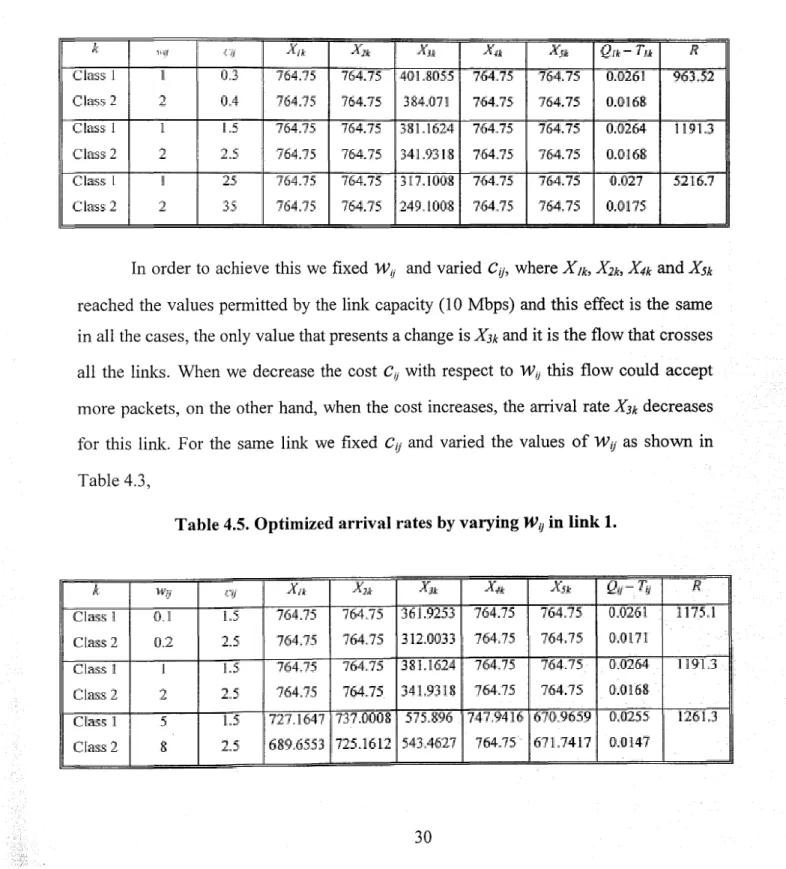
(36) In order to observe the advantage of having the values of the arrival rate optimized and non optimized and how values allow to the service provider calculate the flow of each path and the rebounds in his / her revenue, we increase the value of} above the permissible value for link 1 class 1, see Table 4.2. Table 4.2. Exceeding the capacity in the link 1 class 1. Table 4.3. Rebound in the relationship QoS Delay -. Since some values can saturate me link in a wmie determined tne optimization is becoming very useful so as to know how to allocate the different arrival rate per application and class in an equitable form not allowing that the different arrival rates cause a delay that breaks the values specified in the QoS contract. Taking the values from Table 4.2 it can be observed that the arrival rate for the X~1 classi causes a relationship negative in the penalty in the links crossed by that arrival rate, see Table 4.3. Link 2 is not altered since X~1 does not cross that link.. 29.

(37) We carried out another evaluation to check if it was possible to control the network by the variation of the parameters WI/k and C~ so as to observe if the prices can manage the flow of the paths, we realized this experiment in link 1 since this link is traversed by three of the main flows, X~j, X~3 and X~. The results obtained are shown in the Table 4.2, Table 4.4. Optimized arrival rates by varying C~ in link 1.. In order to achieve this we fixed W~ and varied C~, where X/k, X2k, X4k and X5k reached the values permitted by the link capacity (10 Mbps) and this effect is the same in all the cases, the only value that presents a change is X3k and it is the flow that crosses all the links. When we decrease the cost C,1 with respect to W~ this flow could accept more packets, on the other hand, when the cost increases, the arrival rate X3k decreases for this link. For the same link we fixed C~ and varied the values of W~ as shown in Table 4.3, Table 4.5. Optimized arrival rates by varying W~ in link 1.. 30.

(38) When the utility per link, WI/k is too small compared to the cost C~ in the same link, the rate accepted by the network for the different Xj, X2, X4 and X5 is kept constant and X3 is the only one that varies, where its values for each class decrease. We must mention that in both cases the relation Q,,. —. T,, is positive, therefore we. will not have a loss in revenue when the costs are varied in this form. In the tables 4.4 and 4.5 we carried out the same variations in other link, (link 4), to observe if the effect would remain with no change regardless of the link. The experiment was made in link 4 and the flows that cross that link are X~1, X~3 and X~5, where the results can be observed in Table 4.4, TabLe 4.6. Optimized arrival rates by varvin~ C,, in link 4.. The results followed the same pattern when the cost was varied in this link, i.e., only X3k does not reach the maximum value so as to have all the arrival rates at their maximum capacity Table 4.5 presents the case when the cost is greater than the expected utility per service and it is a hypothetical case since C,1 can never be smaller than WI!. 31.

(39) Table 4.7. Optimized arrival rates by varying W~ in link 4.. The empty columns are due to the violation of the constraint 1a~,>. ..%~. causing a. division per zero in Equation (3.2). We proceed to calculate the average delay per class k in the connection taking the values of the tables 4.3 and 4.4 respectively in order to observe if the variation of the prices and costs can decrease the delay per flow such as the service provider can take a decision of how to put the variables C~ and. so as to manage the delay in the system.. Table 4.8. Average delay per class k in the connection varying W~.. 32.

(40) Table 4.9. Average delay per class k in the connection varying Cy. From Tables 4.8 and 4.9 the service provider can take a decision if he! her can decrease the delay per flow such as he /her does not have problems with a possible loss in the revenue caused by the penalty of the function. It is possible observe that if cy is diminished in relation with wij the delay decreases although no in a significant form. 4 4 Quality of Service variation Since the delay in each link is the only parameter than can cause a decrease in revenue and this penalty will take place if the delay at any link is greater than the necessary QOS per service we proceed to vary both qualities to observe and to compare the revenue when the QoS is varying.. 33.

(41) Figure 4.7. Revenue as a function of QoS for each class.. In Figure 4.7 we present the relationship between the revenue calculated using (3.8), and the Qops for the optimized case (left) and the non optimized case (right), they were made varying the QoS for both classes and were compared by using the cost function at the moment of being optimized and we can see that when the QoS is too strict, the revenue takes smaller values, on the other hand, when the QoS is not so strict, the revenue reaches his maximum value.. 34.

(42) Figure 4.8. Average delay in the network for each class.. We separated the delay in the entire network by observing how the Q0S rebounds in the delay per class. Since the Q0S’s are independent of each other, in Figure 4.8 we can observe that by varying only the QoS of class 1 the delay in class 1 can be affected. When both QoS are too strict the delay in the network is smaller since the traffic in the network is less. The same effect occurs when the QoS of class 2 is being varied at the delay in class 2. In Figure 4.9, we made the same variations and we compared to the sum of arrival rates. The result was the same because when the QoS was too strict and the values of the arrival rates were smaller.. 35.

(43) Figure 4.9. Carried traffic in the network as QoS per class is varied. Figure 4.9 is important, since it tells us the maximum amount of traffic that can be accepted in the entire network given Q0S parameters such that revenue is maximized. This surface can be seen as the constrained traffic capacity of the network since more than that will not be achieved without violating some constraints in the optimization problem.. 36.

(44) Chapter 5 Conclusions and Future work In Chapter 4 we observed and compared the results using our revenue cost optimized and non optimized, where we can notice the next, •. The use of the revenue cost proposed tell us where exactly the level of traffic that produces the maximum revenue in the network is.. •. Logically if the arrival rates are in their maximum capacity the number of packets increases and they can saturate the link capacity very quickly.. •. It must be distinguished the type of traffic before establishing the connection so as to take the considerations of bandwidth and delay required for giving a good service.. •. When we tried to handle the flow paths varying the cost and prices we observed that it was possible to manage any arrival rate, in our specific case (X3k) which was the arrival rate that used more links and the rest of the path flows reached the value permissible by the link capacity.. •. The service provider must take care of the values of each QoS for each class since if he/she does not watch this relationship carefully he/she will have a severe lost in revenue.. During the formulation and evaluation of our model emerging some ideas emerged that can improve it and extend the work, these ideas are mentioned next, •. Consider other models for the nodes different from the M/M!l model, this model needs to have a finite buffer capacity since the QoS depends on buffer size in a great measure.. •. The arrival rates can have another class of distribution since recently researches have demonstrated that the flows in the Internet may be modeled like self-similar traffic processes.. 37.

(45) •. exist a parameter that helps measure the performance in the nodes such as blocking probability.. •. It is necessary to establish a kind of routing that takes into account the parameters used in the revenue cost, such as- the value ofQoS for each class, the cost and prices for using the links, and the delay and number of packets in it-.. There must. 38.

(46) Bibliography [1] Bertsekas D., Gallager R., Data Networks, Prentice Hall, 2 Edition, 1992. [2] Black Uyless, TCP/IP & Related Protocols, McGraw Hill, 2 Edition, 1995. [3] Clark D., “Combining Sender and Receiver Payments in the Internet”, 1996. [4] Cocchi Ron, Estrin Deborah, “A study ofpriority in multiple service class networks”. [5] Courcoubetis C,, Vasilios A., “An approach to pricing and resource sharing for available hit rate (ABR) services”, 1998. [6] Courcoubetis C., Vasilios A., “An evaluation ofpricing schemes that are based on effective usage”, ICC 1998. [7] Kleinrock L.,Communication Nets: Stochastic Message Flow and Delay, Mc Graw-Hill, 1964. [8] Mackie-Mason J. K., Varian H.R., “Pricing the Internet”. [9] Mackie-Mason J. K., Varian H. R., “Some FAQs about Usage-Based Pricing”, 1994. [10] Murphy J., Murphy L., “Bandwidth allocation by pricing in ATM networks”. [11] Stiller B “Accounting, Charging and Pricing of Communication Services”, 1998 ,. [12] Shenker S Clark D “Pricing in Computer Networks Reshaping the Research ,. ,. Agenda” [131Parris Cohn, “A Framework for the Study ofPricing in Integrated Networks” [14] Paxson V., Floyd S., “Why we don’t know how to simulate the Internet”, 1997. [15] Reklaitis G., Ravindran A., Engineering optimization: methods and applications, 2. nd. Edition, 1983. [16] Sairamesh J., Ferguson D., “An approach to pricing, Optimal allocation and Quality of Service provisioning in high-speed packet networks”, 1995. [17] Stallings W, Local and Metropolitan Area Networks, Macmillan, 4th. Edition, 1993. [18] Veciana G., Baldick R., “Pricing Multi-service networks”, 1994..

(47)