Global policy spillovers and Perus monetary policy: Inflation targeting, foreign exchange intervention and reserve requirements

Texto completo

(1)Global policy spillovers and Peru’s monetary policy: inflation targeting, foreign exchange intervention and reserve requirements1 Renzo Rossini,2 Adrián Armas3 and Zenón Quispe4. Abstract This paper provides an overview of the monetary policy actions undertaken by the Central Reserve Bank of Peru, combining its main inflation targeting framework with sterilised FX interventions and reserve requirement measures in order to overcome the spillover effects of global policies to counter the recessionary implications of the global financial crisis. We provide a rationale for the use of these instruments, as well as empirical evidence on their effectiveness. In general, the results show that sterilised FX interventions and reserve requirement changes have the desired effects in limiting spillover effects and smoothing out the interest rate and credit dynamics in a dual monetary economy such as Peru. Keywords: Non-conventional policy, inflation targeting, foreign exchange intervention, reserve requirements JEL classification: E51, E52, E58, F31. 1. The reserve requirement overview and evaluation is based on Armas et al (2014).. 2. General Manager, Central Reserve Bank of Peru.. 3. Manager of the Research Department, Central Reserve Bank of Peru.. 4. Head of Monetary Program, Monetary Policy Design Division, Central Reserve Bank of Peru.. BIS Papers No 78. 241.

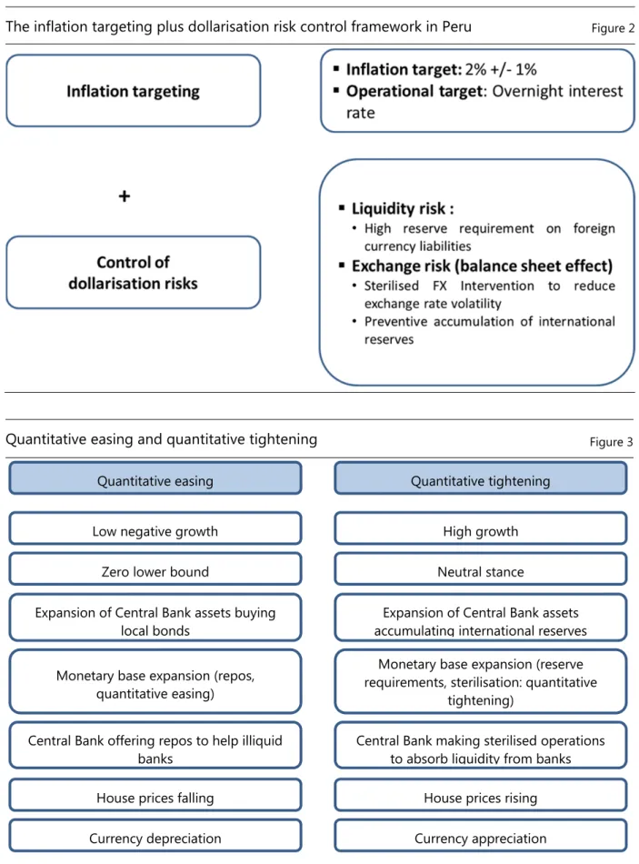
(2) 1. Introduction As a policy response to deal with the macroeconomic challenges brought about by financial dollarisation and its implications for financial vulnerability, the Central Reserve Bank of Peru (Banco Central de Reserva del Perú, BCRP) adopted an inflation targeting (IT) regime in 2002 and became the first monetary authority to implement this framework under a dual monetary system. IT in Peru has a particular design. The BCRP actively intervenes in the FX market to smooth out exchange rate fluctuations and build international reserves as a selfinsurance mechanism against negative external shocks. Since 2008, reserve requirements (RRs) have been used as an active monetary control tool to moderate the impact of capital flows on domestic credit conditions in both domestic and foreign currency. The BCRP has also set high RRs on foreign currency liabilities as a prudential tool to face liquidity and foreign currency credit risk. These additional policy tools have eased the trade-offs that the BCRP faces when implementing standard monetary measures within an IT regime that simultaneously takes into account financial dollarisation considerations. The prompt use of RRs in Peru’s monetary policy framework has allowed the BCRP to induce the necessary quantitative tightening (QT) required to face the domestic spillover effects of the unprecedented quantitative easing (QE) policies implemented by developed countries. This paper describes the relevance of RRs as a complementary instrument for monetary policy based on this experience. The paper is organised as follows: Section 2 provides an overview of Peru’s monetary framework, including the standard interest rate setting; Section 3 evaluates the general implications of the spillover effects of global quantitative monetary policy; Section 4 elaborates on the sterilised FX intervention; Section 5 discusses the use of RRs as a monetary policy tool, the transmission mechanism of RR changes and the control of financial dollarisation risks as well as liquidity risks; Section 6 performs the empirical evaluation of RR policies; and Section 7 concludes.. 2. The monetary policy framework In place since 2002, Peru’s current monetary policy framework is best characterised as a full-fledged IT regime which explicitly takes into account the risks created by financial dollarisation (FD). Figure 1 shows Peru’s high level of financial dollarisation. The inflation target is a 2% annual increase in the consumer price index, with a tolerance band ranging from 1 to 3%. Before the adoption of IT, monetary policy in Peru was implemented through a monetary target framework that used the annual growth rate of the monetary base as an intermediate target and also included instruments such as FX intervention and high RRs for deposits in foreign currency. When IT was adopted, the aforementioned policy tools used to face FD risks remained in place (Figure 2 illustrates Peru’s IT framework). Webb and Armas (2003) and Armas and Grippa (2005) defined the implementation of the IT framework in a financially dollarised economy as a combination of a standard interest rate rule setting plus the active use of other instruments to control financial risks.. 242. BIS Papers No 78.

(3) Dollarisation ratios (Percentage of total). Figure 1. Deposits. Credit 90. 80. 80. 70. 70. 60. 60 50. 2012. 2011. 2010. 2009. 2008. 2007. 2006. 2005. 40.8. 2004. 2013. 2012. 2011. 0. 2010. 0. 2009. 10. 2008. 10. 2007. 20. 2006. 20. 2005. 30. 2004. 30. 2003. 40. 2002. 40. 2003. 40.6. 2002. 50. 2013. 90. Since 2008, RRs have been changed frequently to complement changes in the policy interest rate. The main reason for this new role of RRs was the unprecedented expansionary monetary policies launched in developed economies, which triggered the zero lower bound for their policy interest rates and the implementation of QE. The central banks of emerging economies had to respond with different actions to deal with the spillover effects of these ultra-easy policies, mainly capital inflows and low international interest rates. Figure 3 summarises the different economic cycles and policy responses of both developed and emerging economies during the QE period. Since 2008, changes in the marginal and average RR ratios have been used cyclically in tune with the challenges posed by the new international environment. RRs have been raised in response to capital inflow episodes, such as in Q1 2008, and later on since H2 2010, following the announcement of QE2. RRs were tightened with the aim of offsetting the impact of capital inflows on credit (particularly in dollars), which also gave the BCRP an increased capacity to inject foreign currency liquidity in case of a sudden capital flight. In spite of the country’s high degree of FD, this policy framework has proven to be effective in dampening financial risks. In contrast to what happened during the Russian crisis, when a sudden stop in capital flows triggered a credit crunch, in 2008 the BCRP was better prepared: high international reserves and higher RRs allowed a massive injection of liquidity into the system and prevented another credit crunch.. BIS Papers No 78. 243.

(4) The inflation targeting plus dollarisation risk control framework in Peru. Figure 2. Quantitative easing and quantitative tightening. Figure 3. Quantitative easing. Quantitative tightening. Low negative growth. High growth. Zero lower bound. Neutral stance. Expansion of Central Bank assets buying local bonds. Expansion of Central Bank assets accumulating international reserves. Monetary base expansion (repos, quantitative easing). Monetary base expansion (reserve requirements, sterilisation: quantitative tightening). Central Bank offering repos to help illiquid banks. Central Bank making sterilised operations to absorb liquidity from banks. House prices falling. House prices rising. Currency depreciation. Currency appreciation. Figure 4 illustrates how the use of non-conventional monetary policy tools complements the use of the policy rate. Interventions in the foreign exchange. 244. BIS Papers No 78.

(5) market aimed at offsetting excessive exchange rate volatility reduce systemic risks associated with sharp exchange rate depreciations, whereas the use of high and cyclical RRs in foreign currency contributes to curbing systemic liquidity risks associated with FD.. Peru’s monetary policy framework. Figure 4. International flows of goods and assets. Fiscal policy. Aggregate demand. Inflation. Exchange rate channel Foreign exchange intervention. Exchange rate credit risk Banking lending rates. Policy rate. Reserve requirements. Real interest rates. liquidity risk. Inflation expectations channel. Standard interest rate setting under Peru’s IT (2002–12) The operational target of monetary policy is the short-term interest rate. Like any other central bank with an IT regime, the BCRP uses this operational target to deliver the monetary policy stance to the market. A central bank tends to increase its policy interest rate to fight inflationary pressures during periods of high inflation or output gap levels; conversely, when inflation is below the central bank’s target and the output gap is negative, the central bank tends to cut its policy rate. However, in a financially dollarised economy, the interest rate setting also has to take into account how FD affects the transmission mechanism of monetary policy. The BCRP addresses this issue by using an inflation forecasting model (Modelo de Proyección Trimestral, MPT) that explicitly takes into account the impact of dollarisation on credit market conditions and on the dynamics of the exchange rate and inflation (Winkelried (2013)). In this model, dollarisation reduces the impact of monetary policy on inflation and the output gap, since a large depreciation not only typically generates a positive impact on exports, but also triggers a negative impact on the financial position of firms with currency mismatches. Thus, with FD, the typical expansionary effect of the exchange rate channel after the implementation. BIS Papers No 78. 245.

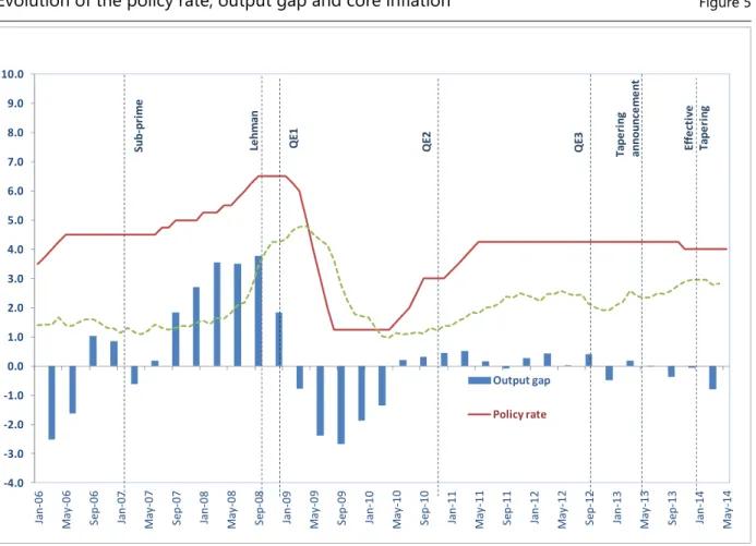
(6) of a policy easing measure is considerably reduced when there is a sharp depreciation. The expansionary net export effect will prevail over the balance sheet effect when depreciation is low. The MPT takes into account the impact of both RR changes and interventions in the foreign exchange market on the dynamics of interest rates and the exchange rate. Figure 5 shows the evolution of the policy rate, the output gap and core inflation since 2004. As we can see, the policy rate has actively responded to the evolution of both inflation and the output gap. In particular, this has been the case in indicators such as core inflation and inflation expectations during episodes characterised by important changes. Estimations of the policy rule for 2002–09 show that it not only meets Taylor’s principle, but also that the central bank gives more importance to reducing inflation volatility than output gap volatility. The estimations reported by Salas (2011) show that the interest rate response to inflation is close to 1.9 and the response to output is close to 0.5.. Evolution of the policy rate, output gap and core inflation. 7.0. Effective Tapering. QE3. QE2. 8.0. Lehman. Sub-prime. 9.0. QE1. 10.0. Tapering announcement. Figure 5. 6.0 5.0 4.0 3.0 2.0 1.0 0.0 Output gap -1.0 Policy rate. -2.0 -3.0. Two episodes highlight clearly the BCRP’s active response to changes in the expected rates of inflation and the output gap. The first started in July 2007, when the central bank began to raise interest rates in response to a persistent rise in inflation. During that period, the BCRP increased its reference interest rate eight times, from 4.5% to 6.5% (a total of 200 basis points). The second episode followed the collapse of Lehman Brothers. The BCRP cut the policy rate aggressively, from 6.5% to 1.25% in six months. The policy rate cuts were effective in reducing interest rates not only in the money market, but also in the rest of the financial system. For. 246. BIS Papers No 78. May-14. Jan-14. Sep-13. May-13. Jan-13. Sep-12. May-12. Jan-12. Sep-11. May-11. Jan-11. Sep-10. May-10. Jan-10. Sep-09. May-09. Jan-09. Sep-08. May-08. Jan-08. Sep-07. May-07. Jan-07. Sep-06. May-06. Jan-06. -4.0.

(7) example, the average interest rate on loans with maturities up to 360 days fell from 15.5% to 11.1% between January and December 2009.. 3. Global policy spillovers and the Peruvian capital market The collapse of Lehman Brothers ushered in the spreading of the subprime crisis to emerging economies, first through higher yields on emerging sovereign bonds, which in the case of Peru were around 10% for a few weeks (Figure 6). That was the first stress test for sovereign bonds, which began to develop in Peru simultaneously with the IT scheme. The QE policy led by the US Federal Reserve in the developed world generated capital flows towards emerging economies, attracted by the nominal rates on domestic Treasury bonds. This trend was clear in Peru from October 2010, with the Fed’s QE2, and then further enhanced by QE3 (Figure 7). For the first time in Peru’s history, the majority of holders of Treasury bonds denominated in domestic currency were foreigners.. Sovereign bond yield curves. Figure 6. Ten-year sovereign bond yield curves: United States and Peru Yield (%). QE3. QE2. 9.0. QE1. 10.0. Lehman. Sub-prime. 11.0. Effective Tapering. Tapering announcement. 12.0. 8.0 7.0 6.0 5.0 4.0 3.0 2.0. Peru. Apr-14. Jan-14. Oct-13. Jul-13. Apr-13. Jan-13. Jul-12. Oct-12. Apr-12. Jan-12. Oct-11. Jul-11. Apr-11. Jan-11. Jul-10. Oct-10. Jan-10. Apr-10. Oct-09. Jul-09. Apr-09. Jan-09. Oct-08. Jul-08. Apr-08. Jan-08. Oct-07. Jul-07. Apr-07. Jan-07. 1.0. United States. In May 2013, with Chairman Bernanke’s hint that the Fed would start tapering its asset purchase programme, the yield on Peru’s 10-year Treasury bonds jumped from around 4% to 6% (Figure 6), with no implications in terms of non-residents’ holdings of Treasury bonds. However, after the tapering process started in January 2014, there were some outflows away from sovereign bonds despite the reduction of the corresponding CDS spreads (Figure 7).. BIS Papers No 78. 247.

(8) 600. Effective Tapering. Tapering announcement. QE3. QE2. QE1. 21 000. Lehman. 24 000. 700. Basis points. Figure 7. 27 000. Sub-prime. PEN millions. Non-residents’ holdings of Treasury bonds and CDS spreads. 500. 18 000 400. 15 000. 300. 12 000 9 000. 200. 6 000 100. 3 000. Non-residents' holdings of Treasury bonds (lhs). May-14. Jan-14. Sep-13. May-13. Jan-13. Sep-12. May-12. Jan-12. Sep-11. May-11. Jan-11. Sep-10. May-10. Jan-10. Sep-09. May-09. Jan-09. Sep-08. May-08. Jan-08. Sep-07. May-07. 0. Jan-07. 0. CDS on Treasury bonds (five-year, rhs). Non-residents’ shift away from Peruvian Treasury bonds did not imply a higher risk for Peru’s economy, as domestic institutional investors absorbed the remaining bonds and the fiscal position was sound (a fiscal surplus of 0.9% of GDP in 2013, the highest in Latin America) and very liquid (public sector deposits at the BCRP amounted to 12% of GDP). The government continued issuing Treasury bonds that were widely accepted by capital markets. The stock of Treasury bonds increased from 6% of GDP in June 2013 to 6.3% of GDP in May 2014 (Figure 8).. Non-residents’ holdings of Treasury bonds. Figure 8. 248. 12. Total holdings / GDP Non–res holdings / GDP. 50. 10. Non–res holdings / total holdings. BIS Papers No 78. May-14. Jan-14. Sep-13. May-13. Jan-13. Sep-12. May-12. Jan-12. Sep-11. May-11. Jan-11. Sep-10. May-10. 0 Jan-10. 0 Sep-09. 2. May-09. 10. Jan-09. 4. Sep-08. 20. May-08. 6. Jan-08. 30. Sep-07. 8. May-07. 40. % of total holdings / GDP and % of non–res holdings / GDP. 14. Effective Tapering. Tapering announcement. QE3. QE1. 60. Lehman. Sub-prime. 70. QE2. 16. Jan-07. % Non–res holdings / total holdings. (In percentages of total holdings and GDP) 80.

(9) 4. Sterilised foreign exchange interventions In the case of Peru, the main purpose of foreign exchange intervention is to reduce exchange rate volatility and accumulate international reserves in order to prevent balance sheet effects, given the partially dollarised financial position of the domestic private sector. Dollarisation magnifies the reaction of financial intermediaries to sharp movements in their funding or high exchange rate volatility. As a result, the economy is prone to credit booms and busts associated with flows of foreign currency deposits, foreign credit lines or other capital flows; and to exchange rate movements affecting the quality of the credit portfolio. Thus, dollarisation distorts the transmission mechanism of monetary policy and increases liquidity and solvency risks within the financial system. Foreign exchange interventions are carried out avoiding any signalling regarding the level of, or a possible ceiling or floor for, the exchange rate. Since the beginning of the BCRP’s interventions under a floating exchange rate system (1990), these operations have been carried out in a discretionary manner. This approach seems to serve Peru’s economy well, as opposed to rules-based intervention.. Foreign exchange intervention. Figure 9. Nominal exchange rate and net foreign exchange market intervention 3.40. 700. Effective Tapering. Tapering announcement. QE3. QE2. QE1. Lehman. 3.20. Sub-prime. 3.30. 900. 500. 3.10 300 3.00 100 2.90 -100 2.80 -300 2.70 -500. 2.60. -700. 2.40. -900 Jan-07 Mar-07 May-07 Jul-07 Sep-07 Dec-07 Feb-08 Apr-08 Jun-08 Aug-08 Nov-08 Jan-09 Mar-09 May-09 Jul-09 Oct-09 Dec-09 Feb-10 Apr-10 Jun-10 Sep-10 Nov-10 Jan-11 Mar-11 May-11 Aug-11 Oct-11 Dec-11 Feb-12 Apr-12 Jul-12 Sep-12 Nov-12 Jan-13 Mar-13 Jun-13 Aug-13 Oct-13 Dec-13 Feb-14 May-14. 2.50. Net FX purchases (USD millions, rhs). Exchange rate (PEN per USD, lhs). Interventions are implemented by purchasing or selling dollars in the spot market and by carrying out swaps and reverse swaps. Swaps and reverse swaps are used mainly when banks might be forced to translate pressures from the non-deliverable forward (NDF) market into the spot market. In this regard, a swap operation with the BCRP can provide temporary coverage against NDF market risks.. BIS Papers No 78. 249.

(10) Latin American nominal exchange rate indices. Figure 10. In highly dollarised economies, it is convenient to build up international reserves to ring-fence the economy against risks associated with FD. Every economic crisis in Peru from the Great Depression and until 1990 was initiated by balance of payments problems. Given that historical background, international reserves as a self-insurance mechanism against international liquidity shortages are a key element of monetary policy design. These cases fall into the category of structural conditions for reserve accumulation. However, the recent need for reserve accumulation is partially associated with important short-term capital flows due to the very accommodative stance of monetary policy in the developed world, which in fact should be considered cyclical. International reserves help a country to preserve economic and financial stability, as they guarantee foreign currency availability in unusual situations, such as possible and significant withdrawals from the financial system or temporary external shocks which could generate imbalances in the real sector and feed back into expectations. Additionally, adequate foreign exchange reserves help to reduce country risk (and improve the associated credit ratings), thereby providing firms with better conditions to access international capital markets. As shown in the BCRP balance sheet, international reserves are funded mainly by public sector deposits and RRs. BCRP securities and currency in circulation also fund the international reserve accumulation, but to a lesser degree. To sterilise the liquidity created by FX interventions, the BCRP issues its own Certificates, currently with maturities of up to 18 months, auctioned on a daily basis, which are complemented by banks’ RRs and Treasury deposits. The following table shows a summary of the 2013 BCRP balance sheet in percentages of GDP, where 11.9% represents sterilisation through Treasury deposits (associated with a solid fiscal. 250. BIS Papers No 78.

(11) position); 11.0% is explained by RRs; BCRP Certificates explain 3.7% of the sources of net international reserves; and currency in circulation accounts for 5.1%.. Balance sheet of the BCRP as of December 2013 (as a percentage of GDP). Table 1. Assets International reserves. Liabilities 31.8. Treasury deposits. 11.9. In domestic currency. 6.7. In foreign currency. 5.3. Reserve requirements. 11.0. In domestic currency. 4.1. In foreign currency. 6.9. Central bank instruments. 3.7. Currency in circulation. 5.1. 5. The use of RRs by the BCRP The BCRP uses RRs mainly for: (a) monetary control, (b) limiting dollarisation risks and (c) increasing the maturity of banks’ external leverage.. a. RRs as an active monetary control tool Non-conventional instruments such as RRs have been used in Peru since the 1990s to preserve the transmission channels of monetary policy and prevent systemic risks associated mainly with exchange rate mismatches and liquidity risks created by FD. The scope and use of RRs have changed in recent years. Before the adoption of IT, and in response to high FD, RRs on foreign currency obligations were higher than on domestic currency obligations. Differential rates seek to encourage banks to internalise the risk of granting dollar-denominated loans to economic agents that do not generate dollar incomes; and to create a foreign exchange liquidity buffer to reduce systemic liquidity risks, given that the BCRP cannot act as lender of last resort (LOLR) in foreign currency. During this period, RRs were not used cyclically and only targeted domestic sources of bank funding. In recent years, RRs have been used by the BCRP as complementary to its short-term interest rate. As such, they have helped to break the trade-off between macro and financial stability. In particular, the RR-induced QT dampened the expansionary effects of capital inflows on domestic credit conditions and, through this channel, also reduced the output gap and inflationary pressures. In the presence of RR policy, this QT effect on the output gap implies that the policy rate may not need to rise as much. Therefore, the use of QT under persistent capital inflows and a still underdeveloped local capital market is analogous to a fiscal policy BIS Papers No 78. 251.

(12) tightening that also allows a lower policy rate and a less appreciated domestic currency; and, as such, introduces a new dimension in the policy mix space, one that must also take into account the relationship between RRs and policy rates.. Reserve requirements in domestic and foreign currency (Percentage of total liabilities subject to reserve requirements). Figure 11. 55. Effective Tapering. Tapering announcement. QE3. QE2. 60. QE1. 70. Lehman. Sub-prime. 80. 50. 49. 50. 40 30. 30. 30. 30 25. 25. 20 16 10. 11.5. Reserve requirement in foreign currency. 6. 6. In addition, under massive capital inflows or very low international interest rates, FD strengthens the spillover from expansionary international monetary conditions to the domestic financial system, which weakens domestic monetary policy. This is so because the demand for credit switches towards foreign currency credit. Under these conditions, higher RRs on dollar liabilities contribute to moderating the spillover effect of international financial conditions on domestic markets, thereby strengthening the transmission of domestic interest rate policy. The use of RRs also contributes to monetary policy effectiveness. In credit market segments where the risk premium is high, lending rates are less sensitive to the policy rate, whereas changes in RRs, which operate through changes in financial intermediation margins, have a larger impact on lending rates. Countercyclical RRs can help to offset credit expansions by reducing the amount of banks’ loanable funds as a proportion of total bank assets. Massive capital inflows until April 2013 due to hitting the zero lower bound in the advanced world (QE, Operation Twist, massive injection of liquidity by the ECB at a rate of 1%, etc) brought about new macroeconomic and financial stability challenges. This time, the pre-emptive use of non-conventional tools by the BCRP helped to create a smoother credit cycle compared with the 2007–08 episode (see Figures 13 and 14). The use of non-conventional policy instruments such as RRs and FX market interventions not only helped to mitigate the foreign currency-induced credit and liquidity risks created by FD, but also contributed to breaking the trade-off between reducing domestic demand pressures and attracting capital flows. The trade-off. 252. BIS Papers No 78. Jul-14. Apr-14. Jan-14. Jul-13. Oct-13. Apr-13. Jan-13. Oct-12. Jul-12. Apr-12. Jan-12. Jul-11. Oct-11. Apr-11. Oct-10. Jul-10. Apr-10. Jan-10. Oct-09. Jul-09. Apr-09. Jan-09. Jul-08. Oct-08. Apr-08. Jan-08. Oct-07. Jul-07. Apr-07. Jan-07. 0. Jan-11. Reserve requirement in domestic currency.

(13) takes place when the policy rate is increased to face domestic demand pressures amid episodes of strong capital flows.. Banking system foreign liabilities (As a percentage of GDP). Figure 12. Effective Tapering. Tapering announcement. QE3. QE2. QE1. 10.0. Lehman. Sub-prime. 12.0. 8.0 Total external liabilities / GDP Short-term external liabilities / GDP 6.0. 4.0. Mar-14. Nov-13. Jul-13. Mar-13. Nov-12. Jul-12. Mar-12. Nov-11. Jul-11. Mar-11. Nov-10. Jul-10. Mar-10. Nov-09. Jul-09. Mar-09. Nov-08. Jul-08. Mar-08. Nov-07. Jul-07. Mar-07. Jul-06. Mar-06. 0.0. Nov-06. 2.0. An increase in the RR ratio implies that banks must raise liquid assets to meet the new policy requirement. This tends to reduce credit growth, particularly when banks cannot replace liabilities subject to RRs with other sources of funding, like long-term foreign liabilities.5 This is more likely the case for small-sized financial institutions with limited access to the international financial markets. Thus, by increasing RRs during episodes of capital inflows and credit expansions, the BCRP seeks to reduce the probability of liquidity stress scenarios in the financial system. Higher RRs induce private banks to increase their availability of liquid assets, which also reduces their capacity to expand credit, particularly in foreign currency. Hence, RRs generate buffer stocks of liquidity in both domestic and foreign currency.. 5. In Peru long-term foreign liabilities are not subject to reserve requirements up to a limit of 2.2 times the bank’s net worth.. BIS Papers No 78. 253.

(14) Banking system domestic currency credit to the private sector and average reserves. 25 Effective Tapering. Tapering announcement. QE3. QE2. QE1. 50. Lehman. Sub-prime. 60. Figure 13. 20. 40 15 30 10 20. 5. 10. Annual growth of credit in domestic currency, lhs. Average reserve requirement in domestic currency, rhs. The quantitative effect of this mechanism depends both on the duration and intensity of RR increases and on the way this policy is implemented. Figure 8 also shows a different behaviour of credit and liquid assets during 2007 and 2008, when credit growth accelerated and liquid assets decreased in spite of the increase in RRs. During this period, the increase in RRs was much milder and shorter-lived than since 2010. The effectiveness of RRs was rather limited during this episode. Also during this period, the increase in RRs was implemented only through rises on marginal rates and not through increases in the average RR ratio. This distinction is important because an increase in the average RR has a stronger impact on banks’ credit supply than an increase in the marginal rate, because the former is not contingent on the growth of bank deposits, as is the case for marginal RRs. Tovar et al (2011) provide empirical evidence on the effectiveness of average over marginal RRs. This implies that when the BCRP increases average RRs, banks must increase their liquid assets even when deposits are not increasing.. 254. BIS Papers No 78. Feb-14. Sep-13. Apr-13. Nov-12. Jun-12. Jan-12. Aug-11. Mar-11. Oct-10. May-10. Dec-09. Jul-09. Feb-09. Sep-08. Apr-08. Nov-07. Jun-07. 0 Jan-07. -.

(15) Banking system foreign currency credit to the private sector and average reserves. 30. 50 Effective Tapering. Tapering announcement. QE3. QE2. 35. QE1. Sub-prime. Lehman. 40. Figure 14. 45. 25. 40 20 15. 35 10 5. 30. -. 25. Annual growth of credit in foreign currency, lhs. Feb-14. Sep-13. Apr-13. Nov-12. Jun-12. Jan-12. Aug-11. Mar-11. Oct-10. May-10. Dec-09. Jul-09. Feb-09. Sep-08. Apr-08. Nov-07. Jun-07. Jan-07. -5. Average reserve requirement in foreign currency, rhs. The transmission mechanism of RR changes RRs affect money and credit conditions through a number of channels. A simple mechanism is described here. As figure 15 shows, RRs first aim at reducing financial entities’ primary loanable funds. Lower loanable funds imply lower liquidity and credit, which in turn has an impact on aggregate expenditure and inflation. This mechanism is more effective when the balance of liquid assets held by financial entities is low. Second, higher RRs reduce banks’ financial margins. Banks will seek to preserve them by widening the spread between lending and deposit rates (León and Quispe (2010), Montoro and Moreno (2011)). They can achieve this by raising lending rates, reducing deposit rates, or both (Terrier et al (2011)). Higher market interest rates induce economic agents to reduce their expenditure, thereby attenuating inflationary pressures. Regarding empirical evidence, there are virtually no references to Peru before 2008, given that RRs were not an active monetary policy tool. The initial approach when the BCRP started to use RRs actively was to calibrate their impact through an accounting procedure that operated through banks’ financial margins (León and Quispe (2010)). In particular, the prior was that the demand for credit was relatively inelastic to changes in the interest rate, mainly for small and medium-sized firms.. BIS Papers No 78. 255.

(16) The transmission mechanism of changes in reserve requirement ratios. Figure 15. Remuneration Financial mark-up. Reserve requirement ratio. Interest rate spread. Interest rates Aggregate demand. Loanable funds Lending and deposits Liquidity position Money multiplier. It was also clear that the effectiveness of the RR tool would depend on the degree of liquid substitute assets or external funding from foreign financial institutions. Data for the 2008–12 events showed that this prior was not far from actual figures. The MPT assumes that changes in this instrument increase bank lending rates. The estimated impact of a 1% rise in the average RR ratio is about 0.3% on average domestic currency lending rates and 0.1% on foreign currency lending rates. The low pass-through from RRs to foreign currency lending rates is explained by the larger set of alternative sources of funding available to corporate firms in foreign currency. In practice, the implementation of monetary policy within a dual currency economy not only requires forecasting of inflation conditional on the policy rate instrument, but also needs a continuous assessment of risks and vulnerabilities created by FD under the baseline scenario. Non-conventional policy instruments are then set to curb those risks. For instance, if the baseline scenario assumes a period of capital inflows and persistent low international interest rates, then two risks arise: (i) the risk of a rapid expansion of dollar-denominated loans; and (ii) a more intense use by local banks of short-term loans from foreign banks. In this case, a rise in RRs on foreign currency liabilities is also considered as a policy option in the baseline scenario.. b. Controlling dollarisation risks with RRs The discussion on the relevance of non-conventional policies as tools to prevent systemic risks and preserve financial stability has become more intense as a result of the international financial crisis. In developed economies, financial asset prices, such as stocks and bonds, are an element in the policy transmission mechanism. In contrast, emerging economies’ shallow capital markets limit the role of financial. 256. BIS Papers No 78. Inflation.

(17) asset prices in the monetary policy transmission. In this group of economies the most important asset price is the exchange rate. This is the case of financially dollarised economies like Peru. FD generates systemic risks on at least two crucial dimensions: first, by reducing the central bank’s ability to act as lender of last resort, FD increases the likelihood of a liquidity shortage in the financial system; and second, since banks lend in foreign currency to non-tradable firms, FD also creates currency mismatches, which magnify foreign currency-induced credit risks. A common feature of these two additional sources of financial vulnerability implied by FD is that both generate negative externalities that justify policy intervention. They can also trigger potential non-linear dynamics with undesirable consequences for financial stability, which supports the introduction of precautionary policy measures. In this regard, the availability of adequate international reserves is key to providing liquidity to the markets during episodes of financial stress. As shown in the BCRP balance sheet (Table 1), the international reserves are funded by deposits from the public sector, RRs, central bank securities and currency in circulation. The key externality at play with FD is a non-pecuniary one (but common before the creation of central banks in the continent). When banks intermediate in foreign currency, they do not take into account the fact that they are operating under a system without a LOLR in that currency. Banks assume that when they need foreign currency they will be able to obtain it from the interbank market (local or international) at the market interest rate (related of course to the policy rate of the foreign currency issuer). However, this may not be the case, particularly if all banks experience the same type of liquidity shortage.. Liquidity risk and LOLR in foreign currency This was the case in Peru during the 1998 Russian crisis. This shock triggered a sudden stop and quickly damaged banks’ foreign currency positions, particularly in those banks that took considerable short-term loans from the international financial system. During this episode, banks were not able to obtain foreign currency even at very high short-term interest rates. As a consequence, several banks had to abruptly curtail credit. The average local interbank rate in dollars was 8% in July 1998 (240 basis points over one-month Libor) and soared to 12.9% in October (760 basis points over one-month Libor). The rationale for high RRs on foreign currency deposits, which strongly emphasises the need to provide adequate international liquidity to the financial system during periods of financial distress, was fundamental in diminishing the impact of the sudden stop during the late 1990s financial crisis. Thus, under FD, preventive policy is required because private banks hold too little foreign currency liquidity. Higher RRs on foreign currency liabilities, jointly with the accumulation of international foreign reserves, contribute to reducing the adverse impact of this externality. A historical reference of a financial system operating without a LOLR (like the FD case) was the 19th century and early 20th century, when bank run episodes were frequent across the world. In the United States, banks were required to keep a 25% reserve against deposits (National Bank Act of 1863). However, the role of RRs decreased over time after the creation of the Fed in 1913 (Goodfriend and Hargraves (1983)). RRs on foreign currency liabilities have three desirable effects that help deal with financial distortions. First, RRs send a signal to financial intermediaries that. BIS Papers No 78. 257.

(18) foreign currency liabilities are riskier than their domestic currency counterparts and, thus, RRs help banks to internalise dollarisation risks. By setting higher RR ratios on foreign currency liabilities, the BCRP increases the cost of providing foreign currency loans, thereby reducing the incentives for banks to intermediate in foreign currency, particularly in those credit market segments where borrowers have few alternative sources of funding. Second, RRs reduce the likelihood of bank runs because economic agents realise that the banking system has a large pool of foreign currency-denominated liquid assets. RRs on foreign currency deposits amount to about 20% of total international reserves, 50% of total foreign currency credit and 44% of overall liabilities subject to RRs. And third, RR policy contributes to increasing the amount of international liquidity in the financial system when necessary. This level of liquidity allows the central bank to act as LOLR in foreign currency by providing it whenever it is needed. By cutting RRs, the central bank can inject liquidity to the financial system and reduce pressures on the interest rate.. Credit risk induced by currency mismatches The existence of currency mismatches in the balance sheet of domestic agents generates an externality to the financial system, because agents either do not properly internalise the foreign currency-induced risk or engage in moral hazard behaviour. Even non-tradable firms which set prices in foreign currency do not realise that the nature of the mismatch is a real one. In other words, a negative shock to the economy that results in a depreciation of the real exchange rate increases the real debt of the non-tradable firm (net present value of cash in dollars will fall). There is also an externality that operates through the payments system: by taking dollar-denominated loans, an individual firm increases its default risk. However, it also increases the default risk of other firms, those that are linked to the first firm through the payments system. Banks do not properly internalise the complex degree of links between firms, and consequently do not charge the right risk premium when granting dollar-denominated loans to firms in the non-tradable sector. In this case, a sharp and unexpected depreciation of the exchange rate can trigger negative balance sheet effects that spill over across the payments system to a large set of firms, unduly affecting the credit quality of banks’ assets. It is worth mentioning that it is not only a sharp depreciation of the domestic currency that generates systemic risks in a financially dollarised economy, but also a strong and transitory appreciation. A persistent and sharp appreciation of the domestic currency reduces the real value of firms’ debt and may also encourage further appreciation expectations. As a result, firms may perceive that borrowing in foreign currency is cheaper, leading them to increase their currency mismatches and, through this channel, the cost of a sudden exchange rate reversal. Policy measures such as additional provisioning for dollar-denominated loans, higher RRs for foreign currency liabilities and FX intervention to smooth out exchange rate fluctuations contribute to dampening this type of credit risk.. c. RRs as an instrument to increase maturities and moderate banks’ external leverage Higher RRs on both foreign currency short-term external liabilities and deposits not only increase the cost of dollar-denominated loans, but also induce banks to lengthen the maturity of their external liabilities and increase the availability of international liquidity. In 2007, the BCRP extended the use of RRs to banks’ short258. BIS Papers No 78.

(19) term foreign liabilities.6 As a result, banks had the incentive to lengthen the maturities of their foreign currency liabilities, which reduced their vulnerability to sudden capital stops. Currently, a 50% special RR is in place for local banks’ obligations to foreign banks with maturities of less than two years. Moreover, banks increased the average maturity of their foreign liabilities from two years in 2007 to four years in 2009. This special RR has also been used cyclically. The BCRP raises its level in periods of abundant capital inflows and reduces it in response to capital outflows. Crucially, after the collapse of Lehman Brothers, the limited exposure of local banks to sudden stops of capital flows allowed banks to maintain their supply of credit, which limited the impact of this shock on the local financial system. More recently, as a result of greater international financial integration and historically low world interest rates, short-term capital flows7 as well as firms’ and banks’ foreign liabilities, particularly bonds, have increased their share in the capital account. In order to limit over-borrowing, the BCRP set an additional RR (i) when the stock of long-term foreign liabilities and bonds exceeds 2.2 times a bank’s net worth; and (ii) when credit growth in foreign currency exceeds a given limit established by the BCRP. Furthermore, in 2013, with the aim of reinforcing credit de-dollarisation, the BCRP introduced additional RRs for financial institutions that grant foreign currency loans above certain prudential limits.. 6. Measuring the effects of RRs In this section we present the effect of RR policy applied to both domestic and foreign currency bank liabilities on interest rates and credit. There has been an active stance in policies aimed at reducing currency and term mismatches in the public sector, as well as in the financial and non-financial private sector. In Table 2, different indicators of vulnerability to external capital account events show that active fiscal and central bank policies have aimed at reducing the impact of credit and exchange rate risks. Econometric evaluation of policy is difficult due to the identification problem. The usual tool in the monetary policy literature is to identify monetary policy through structural VARs. The VAR procedure is sound in a conventional monetary policy setting where the policy rate dynamically interacts with inflation, economic activity and the exchange rate. In the analysis of unconventional monetary policy, it is important to account for episodes of policy interventions characterised by policy on-off situations. For those cases, Pesaran and Smith (2012) propose a policy evaluation exercise where the effectiveness of policy changes can be directly measured. The idea is to compare observed outcomes after a policy change against a counterfactual generated by an econometric forecast conditional on the policy not being implemented. Pesaran and Smith (2012) show that the conditional forecasts can be generated by a reduced-form equation linking outcomes to both policy and controls invariant to policy.. 6. The BCRP had extended the use of RRs to banks’ foreign liabilities in 2004.. 7. NDF forward operations with non-resident investors and purchases of public debt instruments denominated in domestic currency.. BIS Papers No 78. 259.

(20) Indicators of macro vulnerability Unit. 2003. 2008. 2013. Central bank. 1 GDP / NIR. times. 6.0. 4.1. 3.2. 2 M2 / NIR. times. 1.0. 0.9. 1.2. 3 Short−term foreign liabilities + amortisation of external debt / NIR. %. 13.6. 27.0. 12.7. Banking system. 4 Dollarisation of banking credit. %. 76.0. 54.8. 45.3. 5 Short−term foreign liabili es / banking credit. %. 4.9. 5.3. 2.7. times. 3.1. 2.5. 1.7. Public sector. Table 2. 7 Dollarisation of public debt. %. 84.9. 62.5. 44.5. 8 Non−residents' holdings of local public debt / public sector deposits in the CB. %. 0.0. 21.7. 31.0. years. 7.6. 11.2. 12.5. 6 Short−term liabili es (deposits + credit lines) / required reserves. 9 Average maturity of the public debt. All that is required to follow Pesaran and Smith’s (2012) policy assessment exercise is to define outcomes and instruments. The choice must have the special feature that the instrument needs to be “off” and then “on” for a reasonable amount of time. Three such episodes are identified by Armas et al (2014): (i) the increase in the marginal RR for domestic currency deposits from 6% to 25% since July 2010; (ii) the increase in the marginal RR for foreign currency deposits from 30% to 55% since July 2010;8 and (iii) the increase in RRs on banks’ short-term external debt from 30% to 60% since July 2010. According to Pesaran and Smith (2012), what is needed is a reduced-form equation such as:. =. +. +. (1). where is an outcome variable, is the policy instrument, and is a vector of control variables invariant to ad hoc policy changes. The set of outcome variables is given by the levels of outstanding credit denominated in domestic and foreign currency, lending and deposit interest rates in both currencies, and the ratio of short- to long-term external debt of banks. Candidates for control variables include first a set of external variables including the US federal funds rate, the VIX, the trade-weighted US dollar index, the 10-year US Treasury bond yield and the slope of the US yield curve. A second set of control variables comprises variables affected mostly by external conditions (terms of trade, the EMBI, domestic primary output) or by the trend financial development (number of employees, number of branches). The key assumption is that these sets of control variables are invariant to policy. To make inferences, a mean effect quantity is constructed through the following equation:. 8. 260. There was a first tightening episode that started in February 2008 and spanned up to May 2008; however this tightening was quickly reversed after the Lehman collapse, and thus it cannot be used in this exercise.. BIS Papers No 78.

(21) 1. =. −. ). (2). where is the estimated policy coefficient; H is the number of periods over which the specific level of policy tightening has been effective; represents the is the counterfactual observed policy trajectory from period T onwards; and policy trajectory from period T onwards. The number of periods the policy stance lasted is H=22 months. Next, Pesaran and Smith (2012) propose a policy-effectiveness test statistic given by. =. where. ~. 0,1). (3). is the standard error of the policy reduced-form regression. Namely, if the. is relatively large compared to the standard error of the forecasting mean effect equation, then it is likely that the policy effect is significant.. Results The main empirical results of Armas et al (2014) are presented in Table 3. In general, the effect of RR changes that took place in 2010 proved to have indeed increased lending interest rates and reduced deposit rates. The effect on bank interest rates implies that an increase in RRs induces bank interest rate spreads to widen, as described in Section 3 of this paper, and consistent with effects generally expected in the literature (eg Montoro and Moreno (2011), Terrier et al (2011)).. Pesaran-Smith (2012) policy effectiveness statistics Mean effect (. ). Table 3. Policyeffectiveness statistic ( ). p-value. Expected sign. Bank lending rates in domestic currency. 0.001. 6.47. 0.00. yes. Bank lending rates in USD. 0.006. 1.57. 0.06. yes. Bank deposit rates in USD. –0.009. –3.19. 0.00. yes. Bank lending in PEN. –0.019. –0.57. 0.28. yes. Bank lending in USD. –0.008. –0.49. 0.31. yes. Bank’s short-term external debt as a ratio of total external debt. –0.300. 3.20. 0.00. yes. Furthermore, there is evidence that the effect on credit works as expected. This is inconsistent with the results obtained by Pérez and Vega (2014), which show that a 1 percentage increase in the RR ratio has a 0.4 effect on credit growth within six months. The last empirical result presented here relates to the impact of an increase in RRs on banks’ short-term external debt. The evidence provided here is that this. BIS Papers No 78. 261.

(22) policy produced a shift in banks’ external debt towards long-term maturities and away from short-term ones.. Dynamic effects from a 1 percentage point reduction of RRs in domestic currency 3 months Banking sector lending in DC Interest rate spread. 0.26*** –0.07***. 6 months 0.4*** –0.14*. 9 months. 12 months. Table 4 18 months. 0.36. 0.29. 0.18. 0.09. –0.14. –0.14. –0.11. –0.08. * (at 10%), ** (at 5%), *** (at 1%). 7. Conclusions Non-conventional policy tools such as RRs are being used actively by many central banks in emerging market economies. The evidence provided by Peru’s experience shows that this is an effective tool to reduce the trade-offs that expansionary monetary policies in developed economies are creating in emerging market financial systems. In particular, RRs can dampen the credit cycles in periods of capital inflows and reduce their expansionary effects on domestic aggregate demand. Also, when RRs are applied to foreign currency bank liabilities, they can contribute to increasing the availability of international liquidity in the financial system, and consequently help to reduce the impact of capital outflows on the domestic financial system. The paper shows counterfactual exercises made by Armas et al (2014) and following Pesaran and Smith (2012) to quantify the effect of a marginal RR tightening over the period July 2010 to April 2012. The effects on interest rates and credit levels are measured. As with any other form of tax, RRs generate efficiency costs, which can affect the degree of financial development. However, when financial frictions pervade, these costs are of second-order magnitude compared to the benefits of an active use of RRs that reduces the probability of a financial crisis. In this regard, RR calibration needs to take into account these costs to define both the magnitude and the duration of this type of non-conventional policy instrument. In economies like Peru, where domestic capital markets are not well developed, RRs can also speed up the development of these markets by increasing the cost of financial intermediation through the banking system. However, they could also increase the incentives for firms to use more external funding. The aforementioned costs can be reduced by spreading out the burden of prudential regulation among a larger set of instruments, for instance cyclical capital requirements and dynamic provisioning, and, in the case of financially dollarised economies, also additional capital requirements for loans in dollars. The central bank has to continuously assess the efficacy of RRs as prudential instruments and reverse them when necessary. For instance, RRs on short-term bank liabilities were reduced in 2012 for liabilities related to trade finance, so as to avoid a replacement of banking credit with offshore credit lines. Peru’s experience also shows that central banks need to monitor closely the impact of this type of instrument in order to minimise its potential costs. A close coordination with the regulatory authority is also necessary, so as to complement RRs with the use of other instruments aimed at. 262. 24 months. BIS Papers No 78.

(23) reducing systemic risks, such as countercyclical provisioning and capital requirements, as well as a higher capital requirement for foreign loans.. References Armas, A, P Castillo and M Vega (2014): “Inflation targeting and quantitative tightening: effects of reserve requirements in Peru”, Working Paper 003–014, Central Bank of Peru. Armas, A and F Grippa (2005): “Targeting inflation in a dollarized economy: the Peruvian experience”, RES Working Papers 4423, Inter-American Development Bank, Research Department. Castillo, P and D Barco (2009): “Peru: a successful story of reserves management”, in J Izquierdo and E Cavallo (eds), Dealing with an International Credit Crunch. Policy Responses to Sudden Stops in Latin America, IDB. Céspedes, L F, R Chang and A Velasco (2004): “Balance sheets and exchange rate policy”, American Economic Review, 94(4), pp 1183–93. Goodfriend, M and M Hargraves (1987): “A historical assessment of the rationales and functions of reserve requirements”, in M Goodfriend (ed), Monetary Policy in Practice, Federal Reserve Bank of Richmond. Glocker, C and P Towbin (2012): “Reserve requirements for price and financial stability: when are they effective?” International Journal of Central Banking, 8(1), pp 65–114. Montoro, C and R Moreno (2011): “The use of reserve requirements as a policy instrument in Latin America”, BIS Quarterly Review, March. León, D and Z Quispe (2010): “El encaje como instrumento no convencional de política monetaria”, Revista Moneda 143, Banco Central de Reserva del Perú. Mimir, Y, E Sunel and T Taskin (2013): “Required reserves as a credit policy tool”, The BE Journal of Macroeconomics, 13(1), pp 823–80. Moron, E and D Winkelried (2005): “Monetary policy rules for financially vulnerable economies”, Journal of Development Economics, 76(1), pp 23–51. Perez, F and M Vega (2014): “Efectos dinámicos de las tasas de encaje en el Perú”, work in progress, Banco Central de Reserva del Perú. Pesaran, M and R Smith (2012): “Counterfactual analysis in macroeconometrics: an empirical investigation into the effects of quantitative easing”, mimeo, Cambridge University. Terrier, G, R Valdes, C Tovar, J Chan-Lau, C Fernández-Valdovinos, M GarcíaEscribano, C Medeiros, M-K Tang, M Vera-Martin and C Walker (2011): “Policy instruments to lean against the wind in Latin America”, IMF Working Paper 11/159. Tovar, C, M García-Escribano and M Vera-Martin (2012): “El crecimiento del crédito y la efectividad de los requerimientos de encaje y otros instrumentos macroprudenciales en América Latina”, Revista Estudios Económicos 24, pp 45–64. Rossini, R, Z Quispe and E Serrano (2013): “Foreign exchange intervention in Peru”, BIS Papers, no 73, Bank for International Settlements.. BIS Papers No 78. 263.

(24) Rossini, R, Z Quispe and D Rodríguez (2011): “Capital flows, monetary policy and forex intervention in Peru”, BIS Papers, no 57, Bank for International Settlements. Webb, R and A Armas (2003): “Monetary policy in a highly dollarized economy: the case of Peru”, in P Ugolini, A Schaechter and M Stone (eds); Challenges to Central Banking from Globalized Financial Systems, International Monetary Fund. Winkelried, D (2013): “Modelo de Proyección Trimestral del BCRP: actualización y novedades”, BCRP, Revista de Estudios Económicos 26, pp 9–60.. 264. BIS Papers No 78.

(25)