Self-employment and Okun’s Law
relationship: the Spanish case
María Sylvina Porras
*Universidad de la República, Uruguay
Ángel L. Martín-Román
†Universidad de Valladolid, Spain
Abstract
The present research provides evidence on the determinants driving the differences in the unemployment-output relationship in Spanish regions. We followed a two-step approach. First, we estimated a set of time-varying Okun’s coefficients (rolling-window) for the autonomous communities in Spain (1981-2013) showing significant regional differences as well as important changes over time. At the second step, we estimated FMOLS and DOLS models to explain regional differences in Okun’s law. The results obtained lead to the conclusion that differences in the weight of self-employment and its variations over time prove relevant when accounting for differences in Okun’s law between Spanish regions, and its effect (in standard deviations) is greater than that of variations in labour productivity per worker, which so far had been considered the main driver of regional discrepancies. The economic policy implications of this outcome are huge due to the fact that Spanish regional and national authorities are promoting self-employment.
Keywords
Okun’s Law, self-employment, unemployment, GDP, Spanish regions.
JEL Codes
C23, R11, R23, E24, J64
Acknowledgements: The authors are grateful to Francisco Cabo as well as to participants at the XII Jornadas de Economía Laboral for their comments to an earlier draft. The second author was partially supported by the Spanish Ministry of Economy and Competitiveness under project ECO2014-52343-P.
*Instituto de Economía. Joaquín Requena 1375, CP 11200, Montevideo, Uruguay. sylvina@iecon.ccee.edu.uy
†Facultad de CC. Sociales, Jurídicas y de la Comunicación., Plaza del Alto del León de Castilla, 1, 40005
2
1. Introduction
The considerable regional disparity in how unemployment reacts to economic growth (Okun’s Law) reported amongst Spanish regions is an issue that has attracted the research interest of certain authors (Villaverde and Maza, 2007 and 2009). It is logical since the vastly differing unemployment rates amongst the various autonomous communities means that regional factors should be taken account of when devising economic policies aimed at solving the unemployment problem.1
As a “rule of thumb”, Okun’s law is a fundamental empirical relation for policy-making decisions and is a key tool in anticipating the consequences of some of these policies. As a result, gaining an insight into the determinants of such a relationship is a major goal of devising economic policy. In this vein, the main goal of the present research is to gain a deeper understanding of the determinants underlying the differences in Okun’s coefficients in Spanish regions.
Prior literature has shown that, in Spain, the different growth rates in labour productivity amongst regions are an important factor explaining regional differences in Okun’s law (Villaverde and Maza, 2009). In this article, we provide empirical evidence of another factor that is quantitatively more important than the former for explaining such differences: the weight of self-employment.
This is justified since in many instances self-employment is a “refuge employment”, showing countercyclical behaviour or weakly pro-cyclical. In the presence of a high level of self-employment, the destruction of salaried employment during economic downturns will have weaker effects on the aggregate unemployment rate. In addition, the effects on unemployment will be weak if workers leaving self-employment take up salaried jobs created during economic upturns. Such situations will lead to a weak unemployment-output relation.
In fact, since the Spanish government and, at a higher instance, the European Union itself are promoting initiatives to encourage self-employment, it becomes very important to know if such kind of work has a significant influence on Okun’s law. In the case of Spain, a country with a high unemployment rate, laws have been passed to change the legislation governing self-employment: “Encouraging self-employment, both individually and collectively, has been one of the main focuses of the policies
implemented over the last few years in the area of employment.” (Law 31/2015 of 9
September 2015).
The article is organised as follows. Section 2 provides the background to Okun’s law and self-employment. The methodology used in the research is presented in section 3, and the data in section 4. Section 5 provides the empirical results, and the main conclusions are given in section 6.
1 Autonomous communities are an administrative division of the Spanish territory at NUT 2 level.
3
2. Background
2.1. Okun’s law
The existence of an inverse and statistically significant relation between unemployment and output was established by Arthur Okun (1962) in a study conducted for the United States (1947:2 - 1960:4). He used three different specifications of the law and concluded that for each one percent of real GDP growth, the unemployment rate would fall by 0.3 percentage points (pp), once productivity gains and the labour force growth had been taken into account. Such finding had important implications since it provided an approximate measure of the cost in output terms of high levels of unemployment and, at the same time, offered a mechanism to evaluate policies in terms of their impact on unemployment. It is worth pointing out that Okun interpreted the relation in both directions, from output to unemployment and from unemployment to output. He even used the inverse of the estimated coefficient to indicate that for each pp the US unemployment rate rose above its natural level (estimated to be 4%), output moved away from its potential level by around 3%. This led to the use of the estimated coefficient in both directions (the obtained value and its inverse) in subsequent research, and also to the estimation of the Okun’s law with GDP as the dependent variable.2
Based on Okun’s pioneering work, the topic was embraced by economic policy debate and has been the subject of ongoing inquiry on the economic research agenda. Some scholars have focused on ascertaining to what extent it is valid for other countries or regions outside the USA, replicating some of the original versions of the law or questioning some of the aspects involved in the original versions or seeking to explain differences between countries, regions or to account for changes over time. The international economic crisis which began in late 2008, with devastating consequences in terms of job losses and a sharp rise in unemployment in certain countries, particularly Spain, sparked a fresh political and scholarly debate concerning the degree to which said law and its determining factors are valid, with the issue coming once more to the fore at an international scale (Dalyet al, 2014, Ballet al, 2013, Daly and Hobijni, 2010, amongst others).
Labour laws or labour institutions are often cited in the literature as determining factors to account for differences between countries or time variations of Okun’s coefficient. This is because they may impose certain rigidity in the labour market and pose a greater obstacle to adjust employment and thereby influence the impact of output growth on unemployment (Blanchard, 1997, Sögner and Stiassny, 2002 and Balkrishnan, et al., 2010).
At a regional level, research on Okun’s law has only emerged quite recently, with the relation in most cases being estimated from unemployment to output, and
2
4
focusing on ascertaining to what degree the law applies in territorial units below the national scale. Only on rare occasions, an effort has been made to provide an explanation for the regional pinpointed differences.
The pioneering study is Freeman (2000), who explored Okun’s relation in eight regions of the United States, finding support for it in all cases but without significant differences among regions. Nevertheless, in a recent study also for the United States, Guisinger et al. (2015) do find regional differences in Okun’s law when it is estimated for the 50 states. They point out that the high level of regional aggregation used by Freeman (2000) is most likely the reason why regional differences disappear. On the other hand, in a study into eight regions in Greece, Apergis and Rezitis (2003) report that only in two regions were the estimated coefficients significantly different to those in the remaining regions, while Christopoulos (2004) verifies Okun’s relation in six of thirteen Greek regions, reporting major differences among them. It should be also pointed out that the coefficients estimated by Christopoulos differ substantially from those of Apergis and Rezitis (2003), which might be due to the different methodological approach they adopt.
Adanu (2005) estimates Okun’s coefficient for ten regions of Canada and finds that the greatest estimated cost of unemployment in terms of real GDP loss is mostly located in the larger and more industrialised regions. In a study using French data, Binet and Facchini (2013) obtain a significant Okun’s relation for 14 of the 22 regions analysed. They find that a common factor in the regions where the law does not hold is a high percentage of public employment. Durech et al. (2014) study the law for 14 regions of the Czech Republic and eight regions of Slovakia, with the findings evidencing disparities: i) regions where the law was confirmed regardless of the estimation method, ii) those in which it was never confirmed or only weakly so, and iii) those which yielded mixed results. Based on these findings, they report that the law does not appear to be statistically significant in regions that evidence high long-term unemployment rates and low levels of economic growth. These regions are also characterised by their low levels of domestic and external investment.
5
unionization, and a higher share of non-manufacturing employment) drive most differences in Okun's coefficient across states. However, they show that Okun’s relationship is not stable across specifications, which might lead to inaccurate estimates of the potential determinants of Okun’s coefficient.
As regards studies analysing Okun’s law in Spanish regions, Pérez et al. (2003) estimate the relation for Spain and Andalusia and find that cyclical unemployment is less sensitive to the output cycle in Andalusia than in the Spanish economy as a whole, suggesting the possible existence of differences in the said relationship among the various Spanish autonomous communities. Villaverde and Maza (2007 and 2009) estimate Okun’s coefficient (from unemployment to output) for Spain and its 17 regions, finding that they are quite diverse. They point out that this is related to the different growth rates in labour productivity observed in the regions. In a more recent study, Melguizo (2015) finds significant differences in the relationship at the provincial level in Spain. This seems to suggest that taking into account a greater territorial division (50 provinces instead of 17 regions) also merits inquiry. Finally, the results obtained in Clar-López et al. (2014) offer additional elements concerning the relative importance of studying Okun’s law at the regional level in Spain, since it finds that using this relationship enhances the forecasting ability of the econometric models so as to predict the unemployment rate in most regions.
2.2. Self-employment, business cycles and Okun’s law
No evidence has been found connecting self-employment and Okun’s law. Nevertheless, the inherent features of self-employment, and its different evolution compared to salaried employment suggest a link between them. This paper provides empirical support for an important association linking unemployment-output sensitiveness and the relative weight of self-employment within the total employment.
Self-employment embraces a wide range of heterogeneous workers, with diverse degrees of working conditions and economic self-sufficiency. These might be business people who run firms and employ other staff, business people with or without business premises and without paid employees, professionals, independent workers, workers who have a business contract but with a labour relationship which is similar to dependent work, or family employees who are not paid directly for their work.
Such a disparity means that the ups and downs of economic activity might spark vastly differing effects, both in sign and scale, on the various types of self-employed workers and that, in turn, such effects might differ substantially to those on salaried employment.3 If the predominant effect amongst self-employed is countercyclical or
6
weakly pro-cyclical compared to dependent work, the greater the weight of self-employment in the economy, the less intense the relation between unself-employment and output.4
There is empirical evidence showing how self-employment and paid-employment evolve differently. Congregado et al (2012a) conclude that there is a positive relation between salaried work and the self-employed employing others in the EU-12 countries, at least in the long-term and to quite a generalised extent in the short term. On the other hand, they find that the relationship between self-employed without employees and salaried employment differs across countries. In addition, they also find that the relation between employment and salaried work is dominated by the self-employed without employees.
In Spain, the number of self-employed people working rose by 11.4% between 1980 and 2004, whereas the number of salaried workers grew by 66.8% over the same period. This was due to two opposite effects on employment. The number of self-employed without employees (the majority) fell by 11.4%, whereas those self-self-employed employing others rose by 132.2% (Millán, 2009). The prevalent profile of the self-employed worker in Spain was one without employees, male, over 40 years old, with intermediate academic qualifications, working in retailing, transport, or the hospitality sector (Rodríguez Folgar, 2006, González Morales, 2008 and Millán, 2009).
In many instances, self-employment acts as “refuge” employment. In other words, it is an alternative for salaried workers who lose their job during periods of economic recession. In Spain, Cuadrado et al. (2005) find that self-employment is (weakly) counter-cyclically related to GDP with a lag. Put differently, cyclical GDP movements are followed later and with the opposite sign in self-employment. Ariza-Montes et al. (2013) estimate that at least a subset of individuals who in 2007 chose to be wage-earners would have resorted to self-employment in 2011 when the economic crisis reached its peak. Certain findings in Millán et al (2012) seem to concur with the notion that self-employment plays the role of last resort for low-skilled unemployed workers.
For Congregado et al. (2010a), there are arguments to both support and refute the pro-cyclical nature of self-employment. On the side of the “supporting view”, we might find those factors related to business risk, which would justify the pro-cyclical nature of self-employed entrepreneurship. According to the authors, the counter-cyclical behaviour of self-employment is linked to the notion of “refuge” employment when unemployment is high and the availability of salaried work is low. In addition, an inertia effect could be operating for existing self-employed workers due partly to sunk costs and limited opportunities for alternative employment. Such authors analyse the case of Spain and the United States and reject the pro-cyclicality of self-employment as a
4Parker et al. (2012) find structural changes in the cyclical relation between unemployment, output and
7
whole, although they do find evidence of this in the case of self-employed with employees in Spain. Similar results are found in Congregado et al. (2012b).
In a similar vein, we could mention the results obtained by Golpe and van Stel (2008) when studying the link between self-employment and unemployment in Spanish regions. They find the empirical support of what they call the “entrepreneurial” effect, meaning that having a greater number of business people (entrepreneurs) contributes to generating higher levels of competition which, in the long run, might lead to increases in productivity and less unemployment. They report mixed findings for the “refuge” effect of self-employment. In another study for 23 OECD countries (Thurik et al., 2008), the authors also report evidence to support the “entrepreneurial” and “refuge” effects, with the former seemingly greater than the latter. Congregado et al. (2010b) suggest that during upturns in Spain very few self-employed without employees succeed in finding high-quality salaried jobs, as a result of which the stock of self-employed workers might become too great during downturns, when, additionally, many new individuals try to start businesses according to the “refuge” effect.
If self-employment displays countercyclical or weakly procyclical behaviour and, simultaneously, is the occupation of a large part of the population, the destruction of salaried employment during recessions will be reflected more weakly in terms of increased unemployment. At the same time, the drop in unemployment will be to a lesser extent if some of the jobs created during upturns are occupied by workers who leave self-employment. Situations such as these will lead to a weak unemployment-output relationship.
3. Empirical methodology
We follow a two-step approach. In the first step, we estimate Okun’s coefficients for each Spanish autonomous community in order to confirm the law at the regional level and as an input for the second step. Then, we make use of these estimates as dependent variables in a subsequent econometric regression, testing the power of the weight of self-employment to explain regional differences in Okun’s law.
3.1. First step
Following Blanchard (1997), the first-difference model of Okun’s law is:
(1)
where ut is the unemployment rate, gyt the output growth rate at time t and its
8
“normal” output growth rate would be determined by the labour supply and labour productivity “normal” growth rates. Since is unknown, the following model is estimated:
(2)
where is the random error of the model and is a constant equal to – indicating the linear trend of the unemployment rate. As a result, can be estimated based on the
following expression: . As we are working with the first difference in the unemployment rate and we measure the economic activity as a growth rate, both variables are expected to be stationary.5 The estimation can thus be carried out using Ordinary Least Squares (OLS).
In order to measure the variation of Okun´s coefficient in the Spanish regions, we make use the so-called rolling regression or rolling window technique. We estimate the Okun's law for each region over a “continuum” of sample periods (15-year windows). If the relationship were stable over time, then the estimated coefficients should be relatively similar from one regression to the next. The first rolling window estimates the coefficients by using the sample period from 1981 to 1995.The sample period is then moved forward one year, and the regression is re-estimated to produce a second set of estimated coefficients using data from 1982 to 1996. This process is repeated again and again until making use of the last window (i.e. data from 1995 to 2013). Thus, we obtain 19 observations of Okun’s coefficient for the 17 Spanish regions ( , with i indicating the region and t the moment in time).
3.2. Second step
The second stage consists of the estimation of explanatory models by applying the macro-panel or long-panel technique. The results obtained in the first step (Okun’s coefficients) become the dependent variable in this second step. This kind of panel is characterised by having few individuals (small N) whose characteristics are observed in T periods, with T > N. In this case, N corresponds to the 17 autonomous communities in Spain and T to the 19 time-varying observations corresponding to the 15-year windows defined in the first step.6 The panel contains the dependent variable ( ) and the explanatory variables: weight of self-employed (SE), and labour productivity growth (lpg). The last variable was included as a control variable since prior literature has shown that it proves relevant for explaining differences in Okun’s coefficient. As a result, the following model is estimated:
(3)
5 Anyhow this assumption will be tested later on.
9
where zi captures unobserved heterogeneity amongst individuals and εit is the random
disturbance term. The coefficient of interest in this model is , which would reflect how much the weight of self-employment explains Okun’s coefficient regional differences and its variations over time. A significant and negative coefficient is expected, which would support the hypothesis that the greater the weight of self-employment in the total number of workers, the lesser the effect of output changes on unemployment.
When estimating long-panel data, it should be borne in mind that this type of panel contains time series. As a result, this type of modelling involves similar problems to those of time series modelling (i.e. non-stationarity, autocorrelation and spurious relations, etc.). The steps to be taken are thus: 1) testing for unit root, 2) testing for cointegration and 3) estimating the model according to the results obtained in the previous steps.
3.2.1. Panel unit root test
In order to investigate the possibility of panel cointegration, we need to verify that all variables are integrated into the same order. With this aim, we have chosen the panel unit root tests proposed by Im et al. (2003)-IPS-, Levin et al. (2002)-LL-, Breitung (2000)-B-, Maddala and Wu (1999) -Fisher-ADF- and Choi (2001) -Fisher-PP-.
The main advantage of these tests is that their power is significantly greater compared to the standard time-series unit root tests because they combine cross-section and time series data increasing in this way the number of degrees of freedom. On the other hand, they allow unobserved heterogeneity to be taken into account. The tests assume an AR(1) process in the variables, and the existence of a unit root based on an ADF type model is shown:
(4)
with being the cross-sectional deterministic component, , with being the autoregressive coefficient of , and the model residuals well-behaved. If
(i.e. ), would have a unit root, and if it would be weakly stationary ( ). Some tests assume a common autoregressive process amongst individuals ( or ), (LL and B). In other words, the null hypothesis is that the series have a unit root, whereas the alternative hypothesis is that all series are stationary. Others tests allow the parameter to differ (IPS, Fisher-ADF and Fisher-PP) and the alternative hypothesis is that at least one of the individual series in the panel is stationary.
10
individual, allowing pi to be different in each case. The IPS test is based on the average of individual ADF unit root test statistics, whose distribution is asymptotically normal under the null hypothesis. On the other hand, Fisher's tests are based on combining the observed significant levels from the individual tests (p-values). More specifically, in the case of Fisher-ADF, the statistic is chi-squared distributed (with 2N degrees of freedom). As for the case of Fisher-PP, the statistic is standard normally distributed.
If the variables have a unit root -I(1)-, in other words, they are not stationary at levels and but are stationary in the first differences, it must be determined whether there is a cointegration relation amongst them (long-term relation), since this affects the procedure for estimating the relation. If the null hypothesis of no cointegration is rejected, the method for estimating the model will consist of finding a stationary relation. If they are not, the series in first differences will have to be used and a VAR type model should be estimated.
3.2.2. Panel cointegration test
Cointegration tests for panel data display the same advantages as already mentioned for panel unit root tests. We applied Kao (1999) and Pedroni (1995, 1999, 2004) cointegration tests methodology, based on Engle-Granger’s two-step cointegration test. The null hypothesis in all instances is that variables are non-cointegrated. Pedroni’s proposal is less restrictive than Kao’s since it allows for considerable heterogeneity. First, the following relation between variables y and x is estimated(in this case with x: x1 and x2), which are assumed to be I(1):
(5)
The parameters αi and δi allow for the possibility of individual-specific fixed effects and deterministic trends, respectively. Under the null of no cointegration the residual eit will also be I(1) and the following model is estimated to check the existence
of unit root:
(6)
Pedroni proposes parametric and non-parametric statistics to test that hypothesis, which takes into account various dynamics to correct problems of autocorrelation. In addition, the tests are classified into two groups: 1) based on pooling the residuals along the within-dimension of the panel, 2) based on pooling the residuals along the between-dimension of the panel. The former has the null hypotheses for cointegrated tests H0:
ρi=1 and the alternative Ha: (ρi=ρ)<1 (homogeneity). The latter allows for the existence
of heterogeneity since Ha: ρi<1. Seven statistics were generated and the decision
criterion to reject the null of non-cointegration was that at least half of the statistics rejected such a hypothesis.
11
Kao’s test assumes δi =0 and homogeneity in the long-run relation ( and ), although it allows heterogeneity in the constant term (αi). The cointegration test is based on DF and ADF-type unit root tests for eit.
3.2.3. Estimating a cointegrated regression in panel data
There are estimation biases when applying OLS to a cointegrated panel in the presence of endogeneity of variables. This makes it difficult to draw inferences since the t-statistics do not follow a t-Student distribution (Kao, 1999). To solve these problems, two estimators are proposed: FMOLS (fully modified OLS) and DOLS (dynamic OLS). The basic idea behind both FMOLS and DOLS estimators is to correct for endogeneity bias and serial correlation and thereby allow for standard normal inference.
Consider the following model:
(7)
The cointegrating relationship between y and X is assumed to be homogeneous across cross-sections and allows for cross-section specific deterministic effects. is a kx1 vector of the slopes, Xit is a kx1 vector of the integrated regressors, is the
individual fixed effect and are the errors in the cross-section. are the errors long-run covariance matrix, is the contemporaneous covariance matrix and is the one-sided long-run covariance
matrix, with .
In order to solve the above-mentioned problems, FMOLS estimates long-run covariance matrix for the model (7) and uses this to correct for endogeneity bias and serial correlation problems, thus allowing doing the standard normal inference when vector is estimated. The DOLS method employs a parametric correction for the endogeneity achieved by augmenting (7) with lags and leads of the Xit as additional
regressors. This correction gives a solution to the endogeneity problem in the regressors, correcting at the same time the correlation between and
4. Data
To estimate Okun’s law in Spanish regions, we used annual data from Instituto
Nacional de Estadística -INE – (National Statistics Institute) database. Information on
unemployment rate was taken from the Economically Active Population Survey (EPA) and on regional GDP from the Spanish Regional Accounts for the period 1980-2013.
12
substantial differences amongst the regions, ranging from 4.9% in Galicia to 17.1% in Andalucía (Table 1). By the mid-1990s, unemployment in Spain had climbed to 24%: Andalucía once again being the region with the highest rate (32.2%) and Navarra at the opposite end of the scale (13.4%). This was followed by a period lasting almost 13 years during which unemployment fell in all regions in Spain. With the exception of Extremadura (13%), Andalucía (12.8%) and the Canarias (10.5%), the unemployment rate fell into single digit figures in the other autonomous communities and stood at 8.3% for the country as a whole. Then, the international financial crisis that started in 2008 and which seriously affected Spain sparked a dramatic rise in unemployment in the following years and led to unemployment rates in 2013 that more than tripled the 2007 rates in most regions.
The regional economic growth rates did not have shown significant cross-sectional differences during the analysed period, particularly after the second half of the 1990s. In the 1980s and the first half of the 1990s, the regional dispersion was greater than in the subsequent years, despite average growth for the whole period did not differ significantly amongst regions (between 2% and 2.9% in most cases). In following years, regional differences in growth rates fell, reaching a minimum between 2004 and 2008.
For the second stage explanatory model, rolling-windows estimations from the first stage of Okun’s coefficients were used as well as information on the relative weight of self-employment from the INE (SE) and regional labour productivity growth (lpg). The last variable was constructed using data on the number of workers and regional GDP.
In line with the INE classification, self-employed workers include: business people with employees (“employers”), people who work on their own (“own-account workers”), member of a cooperative, and family help. In the current research, self-employed workers are deemed to be business people both with and without other salaried employees, who account for some 92% of all the self-employed in Spain. At regional level, the information available from the INE was used for the period 2001-2013. In previous years, the information used was that presented in the appendix charts of the document: “Structure and dynamics of self-employment”, Carlos III University of Madrid, Employment Outlook (Panorama Laboral) 2008, whose source is also the EPA.7
Differences amongst Spanish regions in the weight of self-employment have fallen over the years at the same time as the proportion has tended to decline in almost all the regions in Spain. In 1980, 34% of the population working in Galicia were self-employed, whereas in Madrid the figure was only 11%. Up until the early 90s, regional differences remained unchanged with only minor variations in just a few cases. It was after the second half of the 90s that the weight of self-employment clearly started to drop, with the exception of Madrid. Regional differences also diminished during what
13
was a period of high economic and more evenly spread growth rates amongst the regions. The years of the economic crisis after 2008 led to a slight increase in self-employment in most Spanish regions.
As regards labour productivity, three markedly different periods also emerge: one period with positive growth rates (1980-1994) but with a greater dispersion amongst regions, followed by a downturn in productivity or little growth in many autonomous communities (1994-2007) tending towards a reduction in regional differences, and finally the period spanning the economic crisis in which positive productivity growth rate was recorded in all regions in Spain.
Given that the sequential estimations of Okun’s coefficient reflect the information of 15-year periods, the SE and lpg variables used in the explanatory model also reflect the information for the same period. In other words, the values of the series of each year of the SE variable correspond to the average weight of self-employment in the same 15-year period, and in the case of lpg, correspond to the annualized growth rate (average growth rate measured over a year) for the same period.
1980 1994 2007 2013 1980-1994
1994-2007
2007-2013 1980 1994 2007 2013 1980-1994
1994-2007
2007-2013
Andalucía 17.1 32.2 12.8 36.2 2.6 3.9 -1.7 21.8 20.8 16.0 18.0 2.4 -0.9 2.6
Aragón 8.3 15.4 5.3 21.4 2.6 3.7 -1.3 26.2 23.6 17.0 16.9 2.3 0.5 2.5
Asturias 8.1 18.0 8.4 24.1 2.1 2.6 -2.2 22.9 23.2 18.3 20.4 2.6 0.3 1.7
Baleares 7.9 16.8 7.2 22.3 4.1 3.2 -1.0 22.0 23.4 17.2 19.5 2.5 -1.7 0.6
Canarias 12.1 24.3 10.5 33.7 2.7 3.5 -1.2 19.3 16.7 12.7 14.4 1.2 -1.6 2.6
Cantabria 7.3 20.9 6.0 20.4 2.0 3.0 -2.1 25.1 24.7 17.8 17.1 2.9 -0.8 1.7
Castilla y León 8.3 19.2 7.1 21.7 2.1 2.6 -1.5 29.8 27.9 20.0 21.7 2.8 0.3 2.2 Castilla La Mancha 10.3 16.9 7.7 30.0 2.4 4.0 -1.3 29.0 26.7 17.9 19.7 2.4 -0.1 2.3
Cataluña 12.2 20.9 6.5 23.1 2.5 3.6 -1.5 17.7 17.7 15.4 16.1 2.1 -0.3 2.3
Com. Valenciana 9.6 23.1 8.7 28.1 2.3 3.9 -2.0 19.0 21.7 16.4 18.1 1.8 -0.7 2.5
Extremadura 14.4 26.1 13.0 33.9 3.3 3.4 -1.0 30.8 24.8 18.5 19.2 3.8 -0.2 2.4
Galicia 4.9 18.1 7.6 22.0 1.5 3.1 -1.3 34.3 32.9 20.8 21.9 3.1 1.1 2.5
Madrid 12.1 17.3 6.2 19.8 2.9 4.4 -0.5 11.3 11.1 12.6 12.6 1.9 -0.2 1.9
Murcia 9.7 24.2 7.5 29.0 2.1 4.3 -1.3 20.1 20.8 15.7 16.7 1.9 -0.4 2.5
Navarra 11.7 13.4 4.7 17.9 2.1 3.8 -1.0 21.1 21.5 17.4 16.8 1.6 0.3 2.1
País Vasco 12.2 23.0 6.2 16.6 1.1 3.4 -1.2 13.5 18.7 16.3 15.6 1.7 0.2 1.7
Rioja 5.0 14.1 5.8 20.0 3.5 3.6 -1.7 29.8 27.3 19.6 19.7 3.0 -0.6 2.2
Note: Growth variables are averege annual growth.
Labour productivity
growth GDP growth
Weight of self-employed Unemployment rate
14
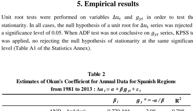
5. Empirical results
Unit root tests were performed on variables and in order to test their stationarity. In all cases, the null hypothesis of a unit root for series was rejected at a significance level of 0.05. When ADF test was not conclusive on series, KPSS test was applied, no rejecting the null hypothesis of stationarity at the same significance level (Table A1 of the Statistics Annex).
5.1. Regional Okun coefficients
Table 2 shows the results of estimating regional Okun’s coefficients for the period 1981-2013. As can be seen, there are significant differences between regions, ranging from a value of -0.18 in La Rioja to -0.91 in Cataluña.
The rolling-windows estimations of Okun’s coefficient also reflect its
differences amongst regions in addition to their evolution over time (Figure 1). In the
gy* = -α / β R2
AND - Andalucía -0.770 *** 2.98 0.708
AR - Aragón -0.586 *** 3.00 0.565
AST - Asturias -0.456 *** 3.09 0.524
BAL - Baleares -0.577 *** 3.67 0.392
CAN - Canarias -0.775 *** 2.91 0.762
CANT - Cantabria -0.539 *** 2.37 0.476
CyL - Castilla y León -0.358 *** 3.04 0.262
CLM - Castilla La Mancha -0.372 *** 3.41 0.593
CAT - Cataluña -0.910 *** 2.63 0.764
VAL - Comunidad Valenciana -0.785 *** 2.94 0.707
EX - Extremadura -0.466 *** 2.19 0.790
GAL - Galicia -0.521 *** 2.67 0.404
MAD - Madrid -0.612 *** 3.17 0.671
MUR - Murcia -0.677 *** 3.03 0.687
NAV - Navarra -0.388 *** 2.83 0.487
PV - País Vasco -0.618 *** 1.94 0.660
RIO - La Rioja -0.179 * 4.61 0.089
Note: * , ** and *** are significant level: 0.10; 0.05 and 0.01 respectively. Table 2
Estimates of Okun's Coefficient for Annual Data for Spanish Regions from 1981 to 2013 : Δut= α + βgyt+ εt
15
left-hand graph, the points corresponding to a particular period represent the estimations of Okun’s coefficient for the 17 autonomous communities for that period. First, a greater dispersion of the coefficients in the early years can be seen, ranging from an absolute value nearly 0 to 1. In other words, unemployment response to GDP growth was very slight or virtually non-existent in certain regions (Castilla y León and La Rioja), whereas in at least one region (Cataluña) the reaction was almost 1 percentage point (pp). This dispersion fell steadily over the years as more updated information was gradually incorporated and older data removed. This graph also shows a general upward trend of the coefficient in absolute value in the middle of the period, indicating a greater response of unemployment to output growth in most Spanish regions, and a certain stability in recent years.
The graph on the right of Figure 1 shows the data distributed by regions, such that the points of the graph corresponding to one autonomous community are the
rolling-windows estimations of Okun’s coefficient for that region for each period from
1981-1995 to 1999-2013. If the points are widely dispersed in one region on the graph, means that Okun’s coefficient experienced significant changes over the analysed period. It is the case of Castilla La Mancha (CM) and Castilla y León (CYL). In other regions, the points are more concentrated, indicating a greater stability in the unemployment-output relationship (Madrid –MAD- and País Vasco -PV-). Furthermore, the graph also reflects regional differences in Okun’s relation. The strong reaction of unemployment to output growth in Cataluña (CAT) contrasts with the slighter reaction in Navarra (NAV).
0 .5 1 1.5 O ku n 's co e ff ici e n t (b e ta ) 1 9 8 1 -1 9 9 5 1 9 8 2 -1 9 9 6 1 9 8 3 -1 9 9 7 1 9 8 4 -1 9 9 8 1 9 8 5 -1 9 9 9 1 9 8 6 -2 0 0 0 1 9 8 7 -2 0 0 1 1 9 8 8 -2 0 0 2 1 9 8 9 -2 0 0 3 1 9 9 0 -2 0 0 4 1 9 9 1 -2 0 0 5 1 9 9 2 -2 0 0 6 1 9 9 3 -2 0 0 7 1 9 9 4 -2 0 0 8 1 9 9 5 -2 0 0 9 1 9 9 6 -2 0 1 0 1 9 9 7 -2 0 1 1 1 9 9 8 -2 0 1 2 1 9 9 9 -2 0 1 3 year
Okun's coef (beta) beta_mean (year)
Distribution by year
Figure 1
Rolling regressions estimates of Okun’s coefficient. Spanish regions (1981-1995 to 1999-2013) (absolute value)
0 .5 1 1.5 O ku n´s co e ffi ci en t (b e ta ) AN D AR
AST BAL CAN
C AN T C YL CM C AT VAL
EXT GAL MAD MUR NAV PV RIO
Spanish regions
Okun's coef (beta) beta_mean (region)
16
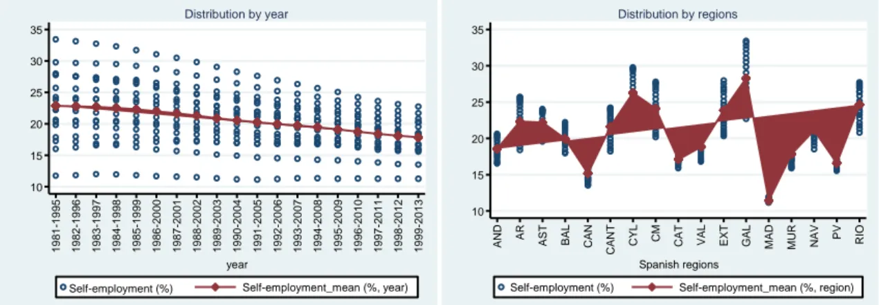
5.2. How much does self-employment explain Okun’s law?
Figure 2 shows the information on the weight of self-employment on total employed, as in the previous figure, in terms of distribution by year or region.
In the figure on the left, we see that regional disparities of the weight of self-employment fell. The mean of the period 1981-1995 was around 11% in Madrid to 34% in Galicia, whereas in 1999-2013 the values were from 11% to 23%. The graph also shows a downward trend in the weight of this type of work in most regions. In the graph on the right, the more dispersed the data points by region, the more change in the weight of self-employment during the analysis period. In Madrid, País Vasco and Cataluña the points are more concentrated, evidencing greater stability. On the opposite side is Galicia.
Figure 3
Okun's coefficient, Self-employmentand Labour productivity growth (variables in means, from 1981-1995 to 1999-2013)
CAT
CAN
BAL VAL AND MUR PV CANT MAD RIO NAV AST CM CyL AR EXT GAL .2 .4 .6 .8 1 1.2 O ku n 's co e ff ici e n t_ me a n (b y re g io n )
-.5 0 .5 1 1.5 2
Labour productivity growth (by region, %)
B. Okun's coefficient and Labour productivity growth
CAT VAL BAL AND MUR MAD CAN PV AR EXT GAL CLM CANT NAV AST RIO CyL .2 .4 .6 .8 1 1.2 O ku n 's co e ff ici e n t_ me a n (b y re g io n )
10 15 20 25 30
Self-employment_mean (by region, %)
A. Okun's coefficient and Self-employment
10 15 20 25 30 35 Se lf -e mp lo ym e n t (% ) 1 9 8 1 -1 9 9 5 1 9 8 2 -1 9 9 6 1 9 8 3 -1 9 9 7 1 9 8 4 -1 9 9 8 1 9 8 5 -1 9 9 9 1 9 8 6 -2 0 0 0 1 9 8 7 -2 0 0 1 1 9 8 8 -2 0 0 2 1 9 8 9 -2 0 0 3 1 9 9 0 -2 0 0 4 1 9 9 1 -2 0 0 5 1 9 9 2 -2 0 0 6 1 9 9 3 -2 0 0 7 1 9 9 4 -2 0 0 8 1 9 9 5 -2 0 0 9 1 9 9 6 -2 0 1 0 1 9 9 7 -2 0 1 1 1 9 9 8 -2 0 1 2 1 9 9 9 -2 0 1 3 year
Self-employment (%) Self-employment_mean (%, year)
Distribution by year
Figure 2
Self-employment. Spanish regions
(Variables in means, % of total employed, 1981-1995 to 1999-2013)
10 15 20 25 30 35 Se lf -e mp lo ym e n t (% ) AN D
AR AST BAL
C AN C AN T C YL CM C AT
VAL EXT GAL MAD MUR NAV PV RIO
Spanish regions
Self-employment (%) Self-employment_mean (%, region)
17
A simple exploratory analysis shows a possible correlation between Okun’s coefficient and employment (Figure 3.A). Regions with the greatest weight of self-employment have at the same time weaker unself-employment-output relationship, which is the hypothesis being tested.
We also included in the model the growth in labour productivity per worker (lpg) since, as already pointed out by other authors (Villaverde and Maza, 2009) and as can also be seen in Figure 3.B., it seems to exist a negative correlation between these variables, so that it might lead to biases omitting it.
As indicated in the methodological section, the estimation procedure first involves testing the stationarity of the panel series and then checking for a cointegration link between the variables. Table A2 of the Annex shows results of unit root tests for panel data applied to the variables: β (Okun’s coefficient), SE (self-employment) and
lpg (growth in labour productivity per worker) at levels and first differences. For the three variables, the results of the tests mostly point to non-rejection of the null hypothesis of a unit root for the series in levels and rejection for the series in first differences.
After not rejecting that series are I(1), cointegration tests for panel data were then applied. As we can see in Table A3, more than 50% of Pedroni’s test statistics indicate rejection of non-cointegration. Kao’s test goes in the same direction; allowing to estimate the long-run relation applying FMOLS and DOLS.
Table 3 shows the results of the estimations. Regardless estimation method, both variables proved significant in all cases for explaining differences in Okun’s coefficient amongst regions and its changes over time and the coefficients took the expected sign.
Pooled estimation
SE -0.05 *** -0.04 ***
lpg -0.12 *** -0.17 ***
R2 0.84 0.94
Weighted estimation
SE -0.05 *** -0.05 ***
lpg -0.16 *** -0.12 ***
R2 0.83 0.94
Notes: Weighted estimation gives estimators for heterogeneous cointegrated panels where the long-run variances differ across cross-sections. * , ** and *** coefficient significant at the 0.01; 0.05 and 0.10 level. SE: Self-employment, lpg: labour productivity growth.
FMOLS DOLS
Table 3 Estimation Results.
18
As can be seen, the estimated coefficient of the SE variable is approximately -0.05, which indicates that for each additional percentage point (pp) of the weight of self-employment, Okun’s coefficient falls by 0.05 pp. This means, for example, that if Okun’s coefficient were 0.8 in absolute value in a region at a given moment in time, it is to be expected (ceteris paribus) that if the percentage of self-employment increases by 1pp, unemployment reaction to output would change to 0.75 pp.
Put differently, if self-employment were the only explanatory variable, regions with the same percentage of self-employment would have the same reaction of unemployment to output. For instance, if Andalucía had had the same weight of self-employment as Asturias in 1999-2013 (approximately 18.5%), Okun's coefficient would be around 0.7 pp in both regions, which was the estimation for Asturias for that period. Nevertheless, as Andalucía had fewer self-employed workers (16.5%) in that period, a greater reaction to output of the unemployment rate should be expected, somewhere around 0.8 pp (the estimation for Andalucía was 0.82).
As expected, the labour productivity growth is also a significant variable to explain regional differences in Okun’s law. The estimated coefficient varies between -0.12 and -0.17. In other words, taking the mean value of the estimations (-0.14), if the difference in growth in labour productivity per worker between two regions were 1pp
(ceteris paribus) the difference in the unemployment reaction to output between said
regions is expected to be 0.14pp. That region showing a greater Okun’s coefficient would display the lowest growth in productivity.
The results obtained reflect a great capacity of SE variable to explain the evolution of Okun’s coefficients and its regional differences. This can be seen by calculating the standardized coefficients of the equation, which provides information on the explanatory power of each regressor:
19
In Table 4, we can see that the variable SE explains to a greater extent than lpg
the differences in Okun’s coefficient. In other words, the expected effect on Okun’s coefficients (in standard deviations) of changes on the percentage of self-employment is 0.302 standard deviations more (0.792-0.490) than the expected by the labour productivity growth rate changes.
6. Conclusions
The present research seeks to gain a greater understanding of the determinants of differences in Okun’s coefficients in Spanish regions, Okun’s law being an important empirical variable for economic policy.
First, Okun’s coefficients were estimated for each region confirming significant regional differences. Values ranged between -0.18 in La Rioja and -0.91 in Cataluña for the whole period. Based on rolling windows estimations we can see a lower dispersion of Okun´s coefficients between regions over the last few periods and an Okun’s relation which has varied significantly over time in certain regions (Castilla La Mancha and Castilla y León) whilst in others, it displayed greater stability (Madrid and País Vasco).
At a second stage, explanatory models of Okun’s regional coefficients were estimated using the macro-panel or long-panel approach. FMOLS and DOLS models were estimated in an effort to test the explanatory power of self-employment of these differences. In line with previous literature, the growth in labour productivity per worker was also included as an explanatory variable. Both variables proved significant in all estimated models.
The results obtained point to a negative relationship between the weight of self-employment and Okun’s coefficients (in absolute value). Then, two regions with a difference of 1pp in the percentage of self-employment should be expected (ceteris
paribus) to have Okun’s coefficients that differ by approximately 0.05 pp. If the
difference in the growth in labour productivity per worker between two regions were
Coefficient
Standard deviation
Standarized coefficient
Okun's coefficient 0.29
SE 0.05 4.56 0.792
lpg 0.14 1.01 0.490
Table 4
20
1pp, (ceteris paribus) the difference in the unemployment reaction to output between said regions would be expected to be about 0.14pp.
Finally, estimating the standardized regression coefficients allows us to conclude that the expected effect on Okun’s coefficients (in standard deviations) of changes in self-employment weight is greater than the expected change due to the effect of changes in labour productivity growth.
References
Adanu, K. (2005). A cross-province comparison of Okun's coefficient for Canada.
Applied Economics, 37, 561-570.
Apergis, N. & Rezitis, A. (2003). An examination of Okun's law: evidence from regional areas in Greece. Applied Economics, 35(10),1147-1151.
Ariza-Montes, J.A., Carbonero-Ruz, M., Gutiérrez-Villar, B. & López-Martín, M.C. (2013). El trabajo autónomo: una vía para el mantenimiento del empleo en una sociedad en transformación, CIRIEC-España, Revista de Economía Pública, Social y
Cooperativa, 78, 149-174.
Ball, L.; Leigh, D. & Loungani, P (2013). Okun's Law: Fit at Fifty? NBER Working
Paper, 18668
Balkrishnan, R.; Das, M. & Kannan, P. (2010). Unemployment Dynamics during Recessions and Recoveries: Okun’s Law and Beyond, World Economic Outlook, Chapter. 3. International Monetary Fund, 69-107.
Barreto, H. & Howland, F. (1993). There are two Okun’s law relationships between output and unemployment. Wabash College Working Paper:
http://web.ntpu.edu.tw/~tsair/2Research/Papers/okun/There%20are%20two%20Okun's %20relationship.pdf
Binet, M.-E. & Facchini, F. (2013). Okun's law in the French regions: a cross-regional comparison, Economics Bulletin, 33(1), 420-433.
Blanchard, O. (1997). Macroeconomics, Prentice Hall, Upper Saddle River, NJ, 384-387.
Breitung, J. (2000). The local power of some unit root tests for panel data. Advances in
Econometrics, 15, 161–177.
Choi, I. (2001). Unit root test for panel data. Journal of International Money and
Finance, 20, 249–272.
21
Clar-Lopez, M., Lopez-Tamayo, J. & Ramos, R. (2014). Unemployment forecasts, time varying coefficient models and the Okun’s law in Spanish regions. Economics and
Business Letters, 3(4), 247-262.
Congregado, E., Carmona, M. &Golpe, A. (2010a). Self-employment and the Business Cycle.: http://www.uhu.es/emilio.congregado/materiales/cyclesspain.pdf
Congregado, E., Golpe, A. A., & Carmona, M. (2010b). Is it a good policy to promote self-employment for job creation? Evidence from Spain. Journal of Policy Modelling,
32(6), 828-842.
Congregado, E.; Carmona, M.&Golpe, A. (2012a). Self-employment and job creation in the EU-12. Revista de Economía Mundial, 30, 133-155.
Congregado, E., Golpe, A., & Parker, S. C. (2012b). The dynamics of entrepreneurship: hysteresis, business cycles and government policy. Empirical Economics, 43(3), 1239-1261
Cuadrado, J., Iglesias, C. & Llorente, R. (2005). El empleo autónomo en España: factores determinantes de su reciente evolución. CIRIEC-España, Revista de Economía
Pública, Social y Cooperativa, 52, 175- 200.
Daly, M.; Fernald, J.; Jorda, O. & Nechio F. (2014). Interpreting deviations from Okun´s law. FRBSF Economic Letter. 2014-12.
Daly, M. & Hobijni, B. (2010).Okun’s Law and the Unemployment Surprise of 2009.FRBSF Economic Letter.2010-07.
Durech, R., Minea, A., Mustea, L. &Slusna, L. (2014). Regional evidence on Okun's Law in Czech Republic and Slovakia. Economic Modelling, 42, 57–65.
Freeman, D. (2000). A regional test of Okun’s Law. International Advances in
Economic Research, 6, 557–570.
Golpe, A.& van Stel, A. (2008). Self-Employment and Unemployment in Spanish Regions in the Period 1979–2001. In E. Congregado, Measuring Entrepreneurship.
Capítulo 9. 191-204.
González Morales, O. (2008). Análisis de las características que distinguen al trabajo por cuenta propia del empleo asalariado. Investigaciones de Economía de la Educación,
3, 329-336.
Guisinger, A., Hernandez-Murilloz, R., Owyang, M. & Sinclair, T. (2015). A State-Level Analysis of Okun's Law. Research Division, Federal Reserve Bank of St. Louis Working Paper Series2015-029A
Herwartz, H. & Niebuhr, A. (2011). Growth, unemployment and labour market institutions: evidence from a cross-section of EU regions. Applied Economics, 43, 4663–4676
Im, K., Pesaran, M. & Shin, Y. (2003). Testing for unit roots in heterogeneous panels.
Journal of Econometrics, 115, 53–74.
22
Levin, A., Lin, C. & Chu, C. (2002). Unit Root Test in Panel Data: Asymptotic and Finite sample Properties. Journal of Econometrics, 108, 1 – 24.
Maddala, G. & Wu, S. (1999). A comparative study of unit root test with panel data y a new simple test. Oxford Bulletin of Economics and Statistics, 61, 631 – 652.
MelguizoCháfer, C. (2015). An analysis of the Okun’s law for the Spanish provinces,
Research Institute of Applied Economics Working Paper2015/01, 1/37
Millán, J.M. (2009).Self-employment: a microeconometric approach. PhD thesis under the supervision of Dr. Emilio Congregado. Universidad de Huelva:
http://rabida.uhu.es/dspace/handle/10272/183?show=full
Millán, J. M., Congregado, E., &Román, C. (2012). Determinants of self-employment survival in Europe. Small Business Economics, 38(2), 231-258.
Millán, J. M., Congregado, E., & Román, C. (2014). Persistence in entrepreneurship and its implications for the European entrepreneurial promotion policy. Journal of Policy
Modeling, 36(1), 83-106.
Okun, A. (1962). Potential GNP: Its Measurement and Significance. Cowles
Commission/Foundation Papers (CFPs), CFP190, 1963.
http://cowles.econ.yale.edu/P/cp/p01b/p0190.pdf
Parker, S. C., Congregado, E., &Golpe, A. A. (2012). Is entrepreneurship a leading or lagging indicator of the business cycle? Evidence from UK self-employment data.
International Small Business Journal,30(7), 736-753.
Pedroni, P (1999).Critical values for cointegration tests in heterogeneous panels with multiple regressors. Oxford Bulletin of Economics and Statistics, 61,653–670.
Pedroni, P. (2000). Fully modified OLS for heterogeneous cointegrated panels.
Advances in Econometrics, 15, 93 – 130.
Pedroni, P (2004).Panel cointegration; asymptotic and finite sample properties of pooled time series tests, with an application to the PPP hypothesis. Econometric Theory,
20, 575–625.
Pérez, J.; Rodríguez, J. & Usabiaga, C. (2003). Análisis dinámico de la relación entre ciclo económico y ciclo de desempleo: una aplicación regional. Investigaciones
Regionales, 2, 141-162.
Rodríguez Folgar, G. (2006). Reseña sobre: “Empleo autónomo y empleo asalariado: análisis de las características y comportamiento del autoempleo en España” de Iglesias, C.; Llorente, R.; Núñez, E. y Cuadrado, J. Ministerio de Trabajo e inmigración, 2004. ISBN 84-8417-147-7. Revista del Ministerio de Trabajo e Inmigración, ISSN 1137-5868, 61, 185-189.
23
Sögner, L. &Stiassny, A. (2002). An analysis on the structural stability of Okun's law--a cross-country study. Applied Economics. 34(14), 1775-1787.
Thurik, A. R., Carree, M. A., Van Stel, A., & Audretsch, D. B. (2008). Does self-employment reduce unself-employment?. Journal of Business Venturing, 23(6), 673-686.
Villaverde, J. &Maza, A. (2007).Okun’s law in the Spanish regions. Economics
Bulletin, 18(5), 1-11.
24
Annex
KPSS test
Statistic p-value Statistic p-value LM-stat
Andalucía - AND -2.7210 0.0084 -3.1010 0.0376
Aragón - AR -3.1464 0.0028 -2.9316 0.0544 0.1313 Asturias - AST -4.1701 0.0002 -4.2846 0.0022
Baleares - BAL -3.2248 0.0022 -3.2444 0.0274 Canarias - CAN -2.9803 0.0043 -3.2200 0.0290 Cantabria - CANT -3.5837 0.0008 -3.3539 0.0214
Castilla y León - CyL -3.3340 0.0017 -2.8822 0.0602 0.0891 Castilla La Mancha - CLM -3.4022 0.0014 -3.5659 0.0131
Cataluña - CAT -2.8891 0.0054 -2.5786 0.1088 0.1353 Comunidad Valenciana - VAL -3.2714 0.0020 -2.7498 0.0781 0.1358
Extremadura - EX -4.7338 0.0000 -4.3704 0.0018 Galicia - GAL -2.8953 0.0053 -3.7942 0.0076
Madrid - MAD -2.7405 0.0079 -2.7240 0.0822 0.1205 Murcia - MUR -2.8909 0.0054 -3.0836 0.0390
Navarra - NAV -3.0189 0.0039 -3.8916 0.0060
País Vasco - PV -3.3469 0.0016 -2.9411 0.0529 0.1556 La Rioja - RIO -3.7098 0.0006 -4.9099 0.0004
Table A1
Unemployment rate
Notes: The ADF tests on unemployment rates were without constant or trend and only with constant on GDP growth. The null (unit root) of ADF tests is rejected if the p-value is below 0,05. The null (serie is stationary) of KPSS tests is not rejected if the stastic is below 0,463 (5%).
Unit Root Test
First difference (∆ut) GDP growth (gyt)
25
Pedroni
Panel v-Statistic 0.3062 -0.6650 Panel rho-Statistic -0.3640 -0.9380
Panel PP-Statistic -1.9657 ** -3.4001 *** Panel ADF-Statistic -3.1047 *** -4.4348 ***
Group rho-Statistic 0.7692 Group PP-Statistic -2.8314 *** Group ADF-Statistic -4.5930 ***
Kao
ADF -2.8129 *** Table A3
Residual Cointegration Test. H0: no cointegration
Statistic Statistic
Statistic
t-Statistic
H1: common AR coefs. (within-dimension)
H1: individual AR coefs. (between-dimension)
Notes: The tests assume "no deterministic trend", but results do not change if assumption is "deterministic intercept and trend". *,** and *** indicates the rejection of the null of no cointegration at 10%, 5% and 1%.
Weighted Method
Null: Unit root (assumes common unit root process) Alternative: all series are stationary
Levin, Lin & Chu t* -1.838 ** -5.816 *** -1.531 * -5.138 *** -5.080 *** -3.435 ***
Null: Unit root (assumes individual unit root process) Alternative: some series are stationary
Im, Pesaran and Shin W-stat 1.041 -6.522 *** 4.890 -5.313 *** -1.771 ** -3.192 ***
ADF - Fisher Chi-square 18.706 106.219 *** 22.338 83.250 *** 43.533 83.250 ***
PP - Fisher Chi-square 22.816 418.438 *** 8.691 66.580 *** 47.340 105.400 ***
Null: Unit root (assumes common unit root process) Alternative: all series are stationary
Levin, Lin & Chu t* 1.512 -5.071 *** -3.033 * -4.377 *** 3.149 -5.749 ***
Breitung t-stat 0.550 -4.433 *** 4.035 0.190 5.081 -2.995 ***
Null: Unit root (assumes individual unit root process) Alternative: some series are stationary
Im, Pesaran and Shin W-stat 0.976 -4.075 *** -3.108 *** -3.250 *** 5.528 -4.527 ***
ADF - Fisher Chi-square 26.509 72.525 *** 66.845 *** 55.733 ** 4.815 55.733 **
PP - Fisher Chi-square 35.671 168.552 *** 49.416 ** 49.148 ** 2.568 136.431 ***
Notes: Probabilities for Fisher tests are computed using an asymptotic Chi-square distribution. All other tests assume asymptotic normality. Total number of observations (NT) ranged between 275 and 306. Estimations undertaken with Eviews 8.0. *, ** and *** indicates the rejection of the null of unit root at 10%, 5% and 1%.
Panel Unit Root Tests (lag length: 1) Table A2
Individual effects and individual
linear trends first diff.
level first diff.
level
Exogenous variables Self-employment (SE)
Labour productivity growth (lpg) Okun's coefficient (β)
Individual effects first diff.