Analysis of the impact of remittances on income distribution in different countries

Texto completo

(1)ANALYSIS OF THE IMPACT OF REMITTANCESS ON INCOME DISTRIBUTION IN DIFFERENT COUNTRIES. AUTHOR: JOSEP FORQUET DOMENECH E-MAIL: [email protected] DEGREE IN ECONOMICS 2014/2015 TUTOR: JOAN ANTONI MARTÍN MONTANER. 1.

(2) ABSTRACT. The analysis of the impact of the remittances allows us to know if remittances have a significant effect on income distribution in the different countries. In this paper we will explain, through the introduction of novel empirical models, if the remittances really have a significant effect and, if they have, what kind of effect it is, positive or negative.. In this essay we will explain firstly a compilation of the most important literature about this topic. Then, we will explain the type of model estimated and the results of the estimation. After that, we will comment the impact of remittances on the different countries.. At the end, our conclusion will be that it is not possible to obtain a single empirical result, because depending on different factors, remittances will affect significantly or not significantly on income distribution in a country. We will also state that, if they are significant, the result is uncertain depending on those factors, this means, they could increase or decrease the inequities on income distribution.. 2.

(3) INDEX 1 1. INTRODUCTION AND LITERATURE REVIEW. ......................................................................5 2. THE ECONOMETRYC ANALYSIS OF THE RELATION BETWEEN REMITTANCES AND DISTRIBUTION OF INCOMES. .............................................................................................. 12 2.1 WHO MIGRATES? ......................................................................................................... 12 2.2 ESTIMATION. ............................................................................................................... 12 2.3 THE SAMPLE. ............................................................................................................... 14 2.4 THE VARIABLES. ........................................................................................................... 14 2.4.1. DEPENDENT OR EXPLANATORY VARIABLES. (GINI'S RATE, 10% AND 20% LOWEST PAID)................................................................................................................................. 14 2.4.2. EXPLANATORY VARIABLES. ....................................................................................... 15 2.4.2.1. CONTROL OR INTEREST VARIABLE (WORKER’S REMITTANCES AND COMPENSATION OF EMPLOYEES, RECEIVED IN % OF THE GDP). .................................................................... 15 2.4.2.2. CONDITIONAL VARIABLES (LEVEL OF DEVELOPMENT AND PUBLIC SECTOR EXPENSES IN EDUCATION AND HEALTH SERVICE)................................................................................ 15 2.5. ANALYSIS OF DATA OF VARIABLES. .............................................................................. 16 3. ESTIMATION RESULTS. ................................................................................................... 20 TABLE 1. ESTIMATION. ....................................................................................................... 22 4. IMPACT OF REMITTANCES ON INCOME DISTRIBUTION.................................................... 28 5. CONCLUSION. ................................................................................................................ 33 6. APPENDIX. ..................................................................................................................... 35 7. BIBLIOGRAPHIC REFERENCES. ......................................................................................... 36. 3.

(4) INDEX 2.. TABLE 1: Countries that receive more remittances………………………………6. TABLE 2: Countries that receive more remittances per capita in terms………6. PICTURE 1: world Gini's rate………………………………………………………..17. TABLE 3: countries with more remittances from emigrants……………………18. PICTURE 2: Map of countries with nominal GDP per capita (1990-2010), according to estimations from IBRD………………………………………………..19. PICTURE 3: map about total expenditure in health service (% of total outlay in health service)…………………………………………………………………………...20. TABLE 4: New definition variables…………………………………………………..28. 4.

(5) 1. INTRODUCTION AND LITERATURE REVIEW. Throughout the years, there have been attempts to explain, empirically, the effect of the remittances, which is the money the emigrants usually send to their country of origin to their relatives, about the distribution of the incomes in different countries or regions, being from the country or urban. Many authors, who will be named and described later, like (Kuznet,1955; Jones,1998; Koechin & Leon,2006) have tried to explain if there is, truly, a significant evidence that the remittances has a positive or negative effect about the distribution of the incomes, that is to say, if it increases the inequality or decreases it. As we will see, the results of the different studies are unalike. The effects are, to some of the authors, positively significant and, therefore, the remittances decrease significantly the inequalities in the distribution of the incomes. But, to some others, the effect is inverse and the inequalities increase notably. To many of the developing countries, the international migrant remittances has become in an important source of external financing in the last two decades. During the last one, the growth of the remittances exceeded to the one of the private capital flow and the foreign public help. According to some estimations of the IBRD (International Bank for Reconstruction and Development,2015), the remittances of the emigrants to developing countries has doubled since 2002 and, in 2007, reached to 251 billion (without the capital flows which are not registered because they go through informal channel. Recent studies of the IBRD (October, 2014) mark that international migrant remittances from developing countries will experience a strong growth in 2015. It is expected to be about 435 billion in 2015, an increase of the 5% regarding the previous year. From a more global view, world remittances, including the one which is destined to the countries which are considered to have high incomes, is calculated in $582 billion in 2014, reaching $608 billion in 2015. As we have said before, remittances is still being a particularly important and stable source of private flows to developing countries, since it takes a huge quantity of foreign currency that helps to keep the balance of payments. In 2013, these deliveries are still being larger than the foreign investment to developing countries (without China), and three times higher than the Official Development Assistance (AOD). Research on remittances (World Bank,2014).. 5.

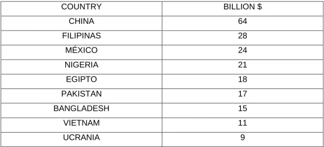
(6) With regard to countries with a higher number of remittances in 2014, we have India, with $71 billion approximately. Other big recipients are:. COUNTRY. BILLION $. CHINA. 64. FILIPINAS. 28. MÉXICO. 24. NIGERIA. 21. EGIPTO. 18. PAKISTAN. 17. BANGLADESH. 15. VIETNAM. 11. UCRANIA. 9. TABLE 1: Countries that receive more remittances As percentage of the GDP (Gross Domestic Product), main remittances recipients were:. COUNTRY. % OF GDP. TAYIKISTAN. 42. REPÚBLICA KIRGUISA. 32. NEPAL. 29. MOLDAVIA. 25. LESOTO Y SAMOA. 24. ARMENIA Y HAITÍ. 21. GAMBIA. 20. LIBERIA. 18. TABLE 2: Countries that receive more remittances per capita in terms Due to these high numbers, to its relative stability in time and to its macroeconomic possible effects, remittances are generating an increasing interest of the international community for these special capital flows. Although the investigation about the impact of the remittances in recipient countries is expanding, the studies which consider the role of these flows in the distribution of the income in the communities of origin are few. Moreover, these studies analysed the effect that the remittances has about the. 6.

(7) distribution of the income in recipients countries, leading, all of them, to contradictory results. Next, we are going to name some of the most important studies about the effect of the remittances in the distribution of the income. All the authors that we are going to talk about now have the peculiarity that, depending on the factors given in migration, remittances may have an equalising effect in the distribution of the incomes or increase the inequalities in the distribution of the incomes. All of them agree that, in the first period of the migration, inequalities increase. Later, when time goes by, this effect disappears and the remittances have the opposite effect. Now, we are going to show you some of the authors who defend the argument that we have exposed before. These authors are: Kuznets was one of the first researchers in analysing the inequalities in the distribution of the incomes and published, in 1955, an article called “Economic growth and income inequality” (Kuznets,1955). It was the first who established two relations with the shape of an inverted U of the Mexican migration. First, the inverted U relates migration rate with the GDP per capita. Second, the inverted U relates the remittances with the inequalities, from a previous relation in which the inequalities are correlated with the migration rate. In this article, he analysed the reasons of the changes in the distribution of the incomes in the long term. His final conclusion was that the distribution of the incomes was having an effect towards equality since 1920 owing to the economic growth. According to Kuznets, the process of the immigration increased the inequalities at the beginning while the country was developing; that is to say, in short and mid-term was all the contrary to the long-term, where the inequality decreased. Empirical analysis that he realised came from historical disagreements between rich and poor people. This author gave two reasons of why the inequality was kept with the passing of time. The first reason was that rich people saved money, since certain studies say that people with high incomes save and the savings of people with lower incomes are close to zero. In the long-term, as it can be deduced, money will be on rich people's hands, since these are who save and the ones who can, as a consequence, increase their wealth. The second reason is the industrialization. The industrialization is a process in which the industry sector increases and decreases the primary sector, that is, the agriculture. Therefore, the distribution of the incomes is reflected on the incomes of the rural and urban population. Having clear that the incomes per capita of the rural population are surely lower than the urban ones, we can conclude that: the more the 7.

(8) participation of the urban population increases, the more inequalities about the distribution of the incomes appear. Moreover, the difference of the incomes per capita between rural and urban population as there is an economic growth, the inequality is kept or even increases, since the productivity per capita in the industrialized sector is higher than in the primary one. Due to these reasons, inequalities increase. Kuznets came to the conclusion that rich people's wealth did not increase because of the cumulative effects of the savings. To come to this conclusion, he gave four reasons: - The State limits the accumulation of property: it does it through direct interventions like taxes to inheritance, or indirect interventions which reduce the value of the assets or limit the yield of the accumulate property. - Demography: the population growth rate between rich and poor people is different; while the proportion of the rich people is reduced because they have less children, the one of the poor people increases because of they have more. - The impact of new industries: technological changes make the assets generated in old industries have, today, less participation to those generated in younger industries. Unless rich people's descendants change their assets to new industries, long-term yields of their assets will be fewer than those more recent. - Service incomes make the participation increases: it is more complicated to later generations of rich people to keep or increase those high level services than to the working class, whose increase is more noticeable. Others of the authors who stand by this stance and is related to Kuznets (1955) are Mc Kenzie and Rapoport (Mc Kenzie & Rapoport; 2004). They argued that international migration is costly and, at first, it can only be afforded by middle and high class' homes, since they can have incentives to emigrate. Therefore, the inequalities in the distribution of the incomes in the community of origin of the emigration will, in this case, increase. Nevertheless, migration networks make the future emigrants' costs drop and, therefore, inequality may decrease. Mc Kenzie and Rapoport show, empirically, that the wealth has not a flat tax in the migration and, subsequently, gives empirical evidence to the relation with the shape of the inverted U between emigration and inequality in rural communities in Mexico. After realising all the estimations, they come to the conclusion just as Kuznets (1955), but 8.

(9) using panel datum with more communities and longer time periods. Migration has an equalising effect on long tradition migratory communities. Following with the authors, we are now going to analyse Jones (Jones, 1998). To him, it is very important to establish a relation between migration and inequality in the incomes, keeping in mind the migration period and the geographical scale. In relation to the first period, Jones came to the conclusion that communities with very low or very high emigration levels (calculated to the level of the community by the percentage of homes with active emigrants or the total of years of migratory experience per home) tend to increase the inequality in the incomes, but those regions where emigration is already in an intermediate period, distributive inequalities tend to decrease. Jones came to the conclusion that those who called them “first innovators” (Innovation Period) of the emigration, tend to come, predominantly, from middle economic sectors, with resources to finance the emigration journey to the United States, and the achieved incomes would allow them to improve their economic position in relation to those who do not emigrate. However, the emigration of the intermediate period (Innovation Period) also suffers changes and migrates those with fewer resources, too. These take advantage of the migration networks and, as consequence, make the remittances more scattered and, therefore, the inequality in the incomes regarding to the first period gets reduced. Finally, when the network system matures in the long term and more homes join the emigration (last period of the innovators), inequalities increase again because homes with emigration represent a significant proportion regarding to homes without migration. This specifies that, if some other previous authors came to different conclusions (some of them argued that emigration generates a bigger inequality (structuralist), while some others came to the conclusion that emigration reduced inequality (functionalist)) was because structuralist people dealt with the first and last period of the innovators and functionalist people dealt with the intermediate period of the emigration. Jones stands up for his position by comparing the inequalities of incomes between four communities in different emigration periods in the center of Zacatecas, which came determined by quantity and antiquity. None of the communities were in the Innovation Period, that is to say, the first period of the emigration. Two of the communities were in the intermediate period, in which Jones divides in phases: I and II. The other two, in the last period of the emigration, were also separated in phases I and II. The final results coincided with their prediction and the inequalities of incomes decreased in the phase I of the intermediate period until phase II period. Subsequently, it increased in the phase 9.

(10) I of the last period, and even more in the second phase of this period. Finally, Jones himself recognised that it was very difficult to trust synchronised datum to prove a many-year process. Other of the authors with this position are Gonzalez-Konig and Quentin Wood (Gonzalez-Konig and Quentin Wood, 2005) who argued that foreign remittances is a key source of incomes in many developing countries, but the impact of this (about how the distribution of the incomes is affected) is not clear. Theoretically, it will depend on who migrates and which is the recipient country of this migration. If emigrant people come from the poorest sectors of the population, the impact of the remittances will probably decrease the inequalities, since poor families are going to receive their salary plus extra incomes from the remittances. On the other way, if migration is produced in the richest part, inequalities tend to increase. The related fact with Jones (1998) is that the impact of the remittances about inequality depends on the period of the migration (3 periods) in the emigrant country. But Gabriel Gonzalez-Konig and Quentin Wodon, unlike Jones (1998), focus on how the impact of the remittances depends on the incomes of the country where remittances is sent. To do so, these authors give a simple model of two periods to explain why the impact of the remittances in the inequality is, a priori, untrue and why the impact of the remittances in the inequality will depend on how the incomes are distributed in the country of origin of the remittances. The first period happens because rich people do not have incentives of emigrating because their income is already high and the poorest people will not be able to emigrate because they exceed their financial possibilities. For this reason, they argue that remittances in the inequality are, a priori, untrue. Regarding to the second period, they expect to demonstrate that depending on the area where the remittances goes, these will have an equalising or differing effect in the distribution of the incomes. To do so, they imagine two homes which migrate: a rural home and an urban one. In the first one, the impact of the remittances will be a decrease in the inequality because it is assumed that the level in urban zones is higher and rich people will not emigrate and have the same incomes. Nevertheless, emigrant families will have additional incomes from the remittances, so this will have an equalising effect in the distribution. The reverse occurs in the home which migrates from rural zones, since these homes are, relatively, poorer than urban homes and hardly any of them can finance the emigration. Therefore, sent remittances (from those few who can afford it) will make the inequality in the distribution in these zones increases. 10.

(11) To demonstrate their empirical model, they used information from a national survey in Honduras. The methodology that they use is the developed one by (Lerman & Yitzhaki, 1985; Sartk, 1986). There, they estimate the impact of the remittances on Gini's coefficient. His prediction of the model confirmed the statements which he had previously described. Continuing with more investigations, following the standard that we have explained before, we find Koechlin and León (Koechlin & León, 2006). They try to verify the hypothesis of the existence of two relations in the shape of inverted U of the Mexican migration from information of the states. Firstly, the inverted U relates migration tax with GDP per capita. Secondly, the inverted U that relates remittances with interpersonal inequality, starting from a previous relation in which interpersonal inequality correlates with the emigration tax. To do so, they analyze 78 countries in the period between 1970 and 2001. These authors come to the conclusion that, at first, remittances has a negative impact in the inequalities of the incomes, but later, as emigration increases, this effect decreases. To finish the literature review, we are going to talk about Acosta (Acosta, 2007). This realises a comparative study of the impact of the remittances and international migration of the poverty and the inequalities in four Latin American countries with important migratory processes (Ecuador, El Salvador, Honduras and Nicaragua). From these home surveys, produced changes in the incomes are estimated throughout the time. He uses a methodology which allows to discompose total changes in two different effects: direct and indirect. Direct effects are related to the effect that the remittances has about the incomes in the homes which participate in the emigration, while indirect effects are the consequences that the remittances has in the participating home and has not any relation with the distribution of the incomes (not observable effects). Results show that the migration and remittances progress reduce the inequalities in the four countries. Poverty taxes are also significantly reduced in Ecuador, El Salvador and Honduras. They argue that emigration has more direct effects if it is realised by a poor home, while if it is realised by a rich home, emigration has more indirect effects. This happens because poor homes give more importance to the incomes than rich homes, where the impact of the remittances is smaller. In summary, empirical studies realised to date do not allow us to know, a priori, if the remittances has the effect of increasing or decreasing the inequalities in the distribution. 11.

(12) of the incomes in recipient countries. The results may be unalike, depending on the factors which are given in the migration.. 2. THE ECONOMETRYC ANALYSIS OF THE REMITTANCES AND DISTRIBUTION OF INCOMES.. RELATION. BETWEEN. 2.1 WHO MIGRATES? At the beginning of the migratory history of a town, when few homes have established contact in a destination of the migration, the remittances' distribution are, necessarily, unequal. When information is hard and scarce, migration is held to a significant grade of uncertainty. The first homes which adopt a migration as an investment will probably be the part of the population with higher incomes, since they are the best equipped to assume a high risk. If the provided remittances to these homes are significant, it may have a notable negative effect in the distribution of the incomes of the town. However, settlers who have successfully migrated provide valuable information that modify parameters which characterise the subjective distribution of the yields to the migration of other villagers. First emigrants can also provide direct assistance to new people. This allows them to adopt a strategy which results a change in the distribution of the yields in their favour (Taylor, 1986). The effect of the remittances in the inequalities depends, in a critical way, on how information and contacts that make the emigration easier, are spread through rural population. If information and contacts are not specific of a home, that is, if there is a tendency to get propagated through family units, then, migration and receipt of the remittances where homes have fewer incomes will be possible. This could revert any unfavourable initial effect about remittances in the inequalities of incomes.. 2.2 ESTIMATION. In this part, we are going to use quantitative evidence to be able to establish the relation between remittances and distribution of the incomes. It is expected to demonstrate if remittances affect the distribution of the incomes in a positive or negative way or, on the contrary, there is no empirical evidence that remittances really affects. To be able to establish a good estimation, different types of variables have been used. We can observe control, conditional and fictitious variables. Control variables are often. 12.

(13) used in macroeconomic level inequality equations (Deininger & Squire, 1997; Calderón & Chonf, 2000; Koechlin & León, 2006, and some others). Just as Kuznets (1955), we are going to establish a relation between remittances (control variable) Gini's rate. The equation will also be composed by a series of conditional variables which provide empirical evidence to the suggested hypothesis. These variables are: the level of development, the expense of the public sector in education, the literacy rate and the expense of the public sector in health service over GDP. The estimated equation will be as follows: GINI= β0 + β1public sector expenses in education over GDP + β2Level of development + β3public sector expenses in health service over GDP + β4 public sector expenses in Education service over GDP + U. Gini's rate measures the quantity of an income and how it is distributed. It does not measure the welfare of a society or allows to determine by itself. It does not measure how the income is extracted or the difference about which countries have better life conditions. Due to this, two more equations with the same explanatory variables will be estimated, but using different explanatory variable. These two variables are: participation in the income of 10% lowest paid of the population and participation in the income of 20% lowest paid of the population in each country. With these variables, we will know how this 10% and 20% of the lowest paid in the income of the population participates, so we will be able to deduce how poor a country is. The other two equations to estimate are: Participation in the income of 10% lowest paid of the population = β0 + β1public sector expenses in education over GDP + β2Level of development + β3public sector expenses in health service over GDP + β4 public sector expenses in Education service over GDP + U. Participation in the income of 20% lowest paid of the population = β0 + β1public sector expenses in education over GDP + β2Level of development + β3public sector expenses in health service over GDP + β4 public sector expenses in Education service over GDP + U.. 13.

(14) 2.3 THE SAMPLE. It will be used a sign of 64 countries (with Appendix), since we have complete information of these countries (corresponding average of a total of three quinquennia). The number of observation will depend on datum availability, but there are, approximately, 700 observations for each variable.. 2.4 THE VARIABLES.. 2.4.1. DEPENDENT OR EXPLANATORY VARIABLES. (GINI'S RATE, 10% AND 20% LOWEST PAID). The first dependent variable is Gini's coefficient. This coefficient is a measurement of the concentration of the income in a region for a certain period. Gini's rate uses values ranging from 0 to 1, where 0 points out that all individuals have the same income and, therefore, there is a perfect distribution of the incomes. 1 indicates that only one individual has all the income and, therefore, the situation is more unequal in the distribution of the incomes. It measures the inequality grade in the distribution of the income or inequality of the wealth of a region. As we have previously commented. It does not measure the welfare of a society, neither allows to determine by itself or how the income is concentrated or the difference about which country has better life conditions. The data of the sample about Gini's rate to realise the estimation of the model has been extracted from IBRD (www.worldbank.com). The second explanatory variable is the participation in the income of the 10% lowest paid of the population. This variable shows the percentage participation in the income or in the consumption is the participation in which subgroups of population are represented in decile or quintile. Quintile percentage participation cannot reach 100%, due. to. round.. The. data. of. the. proof. are. extracted. from. the. IBRD. (www.worldbank.com). Last explanatory variable is the participation in the income of the 20% lowest paid of the population. It indicates the same as the previous one, but including more population, specifically 10% more. The data of the proof are extracted from the IBRD (www.worldbank.com).. 14.

(15) 2.4.2. EXPLANATORY VARIABLES. 2.4.2.1. CONTROL OR INTEREST VARIABLE (WORKER’S REMITTANCES AND COMPENSATION OF EMPLOYEES, RECEIVED IN % OF THE GDP). Workers' remittances and employees' remuneration comprise current transfers which migrant workers, wages and salaries by non-resident workers realise. The data are the sum of three elements explained in the International Monetary Fund's Fifth Balance of Payments Manual. These are the remittances of the workers, the compensation of the salaried and migrant transfers. First, workers' remittances are classified in private transfers (sent by migrant workers who are considered resident of their adopted country for more than a year, regardless of their legal situation of immigration to recipients who are in their country of origin). Secondly, migrant transfers are defined as the net value derived from migrants who are planning to stay more than one year in the adopted country, which is transferred from one country to another in the moment of the migration. Finally, the remuneration of the employees is the income of the migrant people who have lived in the adopted country for less than one year. Our main interest variable is the remittances. The information has been extracted from the IBRD (www.worldbank.com).. 2.4.2.2. CONDITIONAL VARIABLES (LEVEL OF DEVELOPMENT AND PUBLIC SECTOR EXPENSES IN EDUCATION AND HEALTH SERVICE). The first of the conditional variables is the level of development and is measured as a logarithm of the GDP per capita. GDP per capita is the gross domestic product divided by population at the middle of the year. GDP is the sum of the aggregate gross value of all resident producers in economy plus all taxes of the products, except all subsidies which are not included in the value of the products. It is calculated without doing deductions for depreciation, exhaustion or deterioration of natural resources. Information about the level of development has been extracted from the IBRD (www.worldbank.com). Continuing with explanatory variables, we are going to focus now on public sector outlay in education (% of total outlay in education). It is composed by the general government outlay in education (capital flow and transfers) and it is expressed as a GDP percentage. It includes expenditures financed with transfers from international sources to the government. Total public expenses in education (% of GDP) are. 15.

(16) calculated by dividing the government total outlay in all levels of education by part of GDP, and multiplying it for 100. The percentage of public outlay in education regarding to GDP is useful to compare the outlay in education among countries in time, in relation to the size of their economy. A high GDP percentage suggests a high priority for education and ability to increase the incomes for public outlay (www.worldbank.com). Last explanatory variable is public sector outlay in health service (% of total expenses in health service). Public outlay in health service comprises capital expenditure that comes from public budgets (central and local), external indebtedness and donations (included the ones from international organisms and non-governmental organisations) and social and obligatory health's funds. Total expenditure in health service is the sum of public and private outlay in health service. It comprises preventive and curative health services, family planning activities, nutrition activities and urgent assistance designated to health service, but it does not include water supply and health services. Data have been extracted from IBRD (www.worldbank.com). All these conditional variables have in common a relation with Gini's rate. Literacy rate and public outlay in education are related, evidently, to education, an important factor for the development of a country. Per capita GDP is another indicator of the level of development of a country, larger per capita GDP, larger level of development of a country. It happens the same with the public outlay which is destined to health service, a healthier country with a longer life expectancy is a more developed country.. 2.5. ANALYSIS OF DATA OF VARIABLES. Before starting to estimate the model, it is proper to analyse the data of some variables which appear in the model, so we can understand the results of this estimation in a better way. First, Gini's rate will be analysed. After extracting the data of this rate, the results, in a world map, would be as follows:. 16.

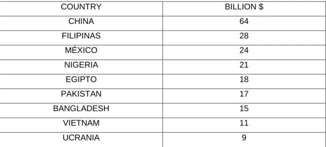
(17) PICTURE 2: world Gini's rate As it may be observed in the map, higher Gini's rates are in Central America, South America and the African continent (where data are available). On the other hand, places with a lower Gini's rate are Canada, Europe and some Eastern countries. This phenomenon may be due to globalisation. Globalisation is an economic, technological, social and cultural global process that consists of communication between different countries of the world and unifying markets, societies and cultures through a series of social, economic and political transformations. All countries which have experienced globalisation have increased Gini's coefficient significantly (China, India, South America...). It is true that globalisation has brought wealth, but only to some, hence, such a large Gini's rate and great inequalities in the distribution of the incomes. One of the reasons of these Gini's rates so high is because economic operators do not invest in their own country, but they speculate and develop their own country in search of own benefits. Other data which must be analysed in detail is remittances. Now, we are going to show a table about the countries with more remittances from emigrants.. 17.

(18) COUNTRY. BILLION $. CHINA. 64. FILIPINAS. 28. MÉXICO. 24. NIGERIA. 21. EGIPTO. 18. PAKISTAN. 17. BANGLADESH. 15. VIETNAM. 11. UCRANIA. 9. TABLE 3: countries with more remittances from emigrants As it may be observed in the table, the volume of money sent by immigrants in remittances to their country of origin increased 6% in 2010, what means $325.000. First recipient countries of remittances are India, China, Mexico and Philippines, according to IBRD. Mexico is the country with the highest number of emigrants (11,4 million) although it is the fourth after Philippines in terms of money received. It is followed by India, second country with more emigrants and with the highest number of money received, close to China. Money is mainly sent from the United States, since there are 42’8 million of immigrants and it is origin of $48300 million sent. It is followed by Saudi Arabia ($26000 million), Switzerland ($19600 million), Russia ($18600 million) and Italy ($13000 million). If we analyse the data of the level of development (per capita GDP), we can observe that there is a lot of difference between countries and even continents in terms of inequality. Now, it will be showed a map of countries with nominal GDP per capita, which is the sum of all goods and final services produced by a country in a year, divided by estimated population in the middle of the same year, which corresponds to data used for the Level of development variable.. 18.

(19) PICTURE 2: Map of countries with nominal GDP per capita (1990-2010), according to estimations from IBRD. +40000. +30000. +20000. +15000. +13000. +10000. +8000. +6000. +3000. +1000. -999. -900. Delimiting great zones and as you can observe, countries with larger GDP per capita and, therefore, higher level of development and better welfare are North America, Europe and Australia. On the contrary, Africa, Asian continent, most of South American countries, Central America and Russia (ordered from a lower to higher GDP per capita respectively) are the zones with a lower GDP per capita, what means they have a lower welfare and level of development. To finish with the analysis of data, we must highlight two indicators which are related to welfare and social development of a country. These indicators are public outlay in education and health service of each country. As we have previously analysed the literacy rate and it has a strong relation to public outlay in education, we are going to focus on public outlay in health service now. As we can see in the following picture, most developed countries are also the ones with more health service expenses. However, there are disagreements about this fact, for example the United States. This is due to the kind of policy of this country, where health service is mostly private. Here, you can observe a map about total expenditure in health service (% of total outlay in health service).. 19.

(20) PICTURE 3: map about total expenditure in health service (% of total outlay in health service).. 3. ESTIMATION RESULTS. To estimate the results, we have estimated for OLS, two types of equations, in which one contains temporary effects and space effects which allows us to consider the heterogeneity of the different countries, and the other equation doesn't contain temporary effects or spatial effects. We will estimate using OLS (Ordinary Least Squares) because it will allow us to know what kind of connection there is between explanatory variables with the dependent variable.. The regressions that we have used to estimate the different models are the following: GINI= β0 +β1REM + β2EDU + β3PIB + β4SALUD +U.. Where GINI is the Gini index, REME is the remittances, EDU is the total spending on education in % of the GDP, per capita is the total expenditure on health in % of GDP and finally GDP per capita GDP. VA10= β0 +β1REM + β2EDU + β3PIB + β4SALUD+U.. 20.

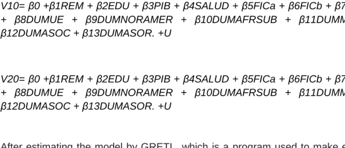
(21) In this regression the difference is the explained variable V10 which is the participation in the income of the lowest paid 10% of the population. VA20= β0 +β1REM + β2EDU + β3PIB + β4SALUD+U.. In this regression, the difference is the explained variable V20 which is the income share of the lowest paid 20% of the population again. GINI= β0 +β1REM + β2EDU + β3PIB + β4SALUD + β5FICaT + β6FICbT + β7DUMSUDAA + β8DUMUEA + β9DUMNORAMERA + β10DUMAFRSUBA + β11DUMMAGREBA + β12DUMASOCA + β13DUMASORA.+U. Where FicaT is a dummy variable of time which takes value 1 when the estimated data are in the first five years (1995-2000) and it takes the value 0 in the other five-years (2000-2005; 2005-2010). FICbT which takes value 1 when the estimated data are in the second half (2000-2005). We have grouped the countries in different regions because we don't have sufficient degrees of freedom to include a fictitious variable which would have been desirable. As result of this group, the different regions are DUMSUDAA which is a dummy variable of geographic area that takes value 1 when the estimated data are of South American regions and 0 when they aren't. DUMUEA dummy variable which takes value 1 when the estimated data are of European countries. DUMNORAMERA dummy variable that takes value 1 when the estimated data are of countries of Central and North America. DUMAFRSUBA dummy variable that takes value 1 when the estimated data are of countries of sub-Saharan Africa. DUMMAGREBA dummy variable that takes value 1 when the estimated data are of countries that belong to the Maghreb (North Africa). DUMASOCA dummy variable which takes value 1 when the estimated data are of countries in West Asia (Central Asia, South Asia and West Asia). DUMASORA dummy variable takes value 1 when the estimated data are of East Asian countries (North Asia, South East Asia and East Asia). Finally, dummy variable DUMUENOA which takes value 1 when the estimated data are of countries that are in Europe but outside the EU. To avoid falling into the trap of dummy, so there is a perfect multicollinearity (the sum of all the fictitious variables is equal to 1) and it can be seen, it is not included in the regression DUMUENOA being this the base group that prevents the fictitious variables sum to 1 and thus avoids falling into perfect multicollinearity.. 21.

(22) V10= β0 +β1REM + β2EDU + β3PIB + β4SALUD + β5FICa + β6FICb + β7DUMSUDA + β8DUMUE + β9DUMNORAMER + β10DUMAFRSUB + β11DUMMAGREB + β12DUMASOC + β13DUMASOR. +U. V20= β0 +β1REM + β2EDU + β3PIB + β4SALUD + β5FICa + β6FICb + β7DUMSUDA + β8DUMUE + β9DUMNORAMER + β10DUMAFRSUB + β11DUMMAGREB + β12DUMASOC + β13DUMASOR. +U. After estimating the model by GRETL, which is a program used to make econometric estimations, the results are:. TABLE 1. ESTIMATION. It includes those two regressions that we've seen before and which have a GINI explained variable.. VARIABLES. 1° COEFICIENTE 50,301 (20,921) -0.271 (-2.564) -0.5314 (-1.048) -0.0001 (-3,134) -0,111 (-2,631). REGRESION VALOR P. FICaT. -. -. FICbT. -. -. DUMSUDAA. -. -. DUMUEA. -. -. DUMNORAMERA. -. -. DUMAFRSUBA. -. -. DUMMAGREBA. -. -. DUMASOCA. -. -. DUMASORA. -. -. R-CUADRADO R-CUA CORRE. 0,181303 0,16501. -. CONSTANTE REM EDU PIB SALUD. <0.00001*** 0,01231 ** 0,29852 0,00196 *** 0,00918 ***. 2° COEFICIENTE 36,185 (13,433) 0.021 (0.371) 0,362 (0,124) -6.860E-0.5 (-1,514) -0,020 (0,865) 0,140 (0,142) 0,021 (0,031) 18,366 (9,921) -2,698 (-1,551) 12,957 (7,501) 9,823 (5,033) 1,354 (0,562) -1,495 (-0,802) 2,533 (1,294) 0,70249 0,68459. REGRESION VALOR P <0,00001 *** 0,71216 0,71655 0,13199 0,38947 0,88217 0,97623 <0,00001 *** 0,12117 <0,00001 *** <0,00001 *** 0,57382 0,42144 0, 19746. *** Significant variable at a significance level of the 10%, 5% or 1% variable.. 22. -.

(23) As can be seen in the table, in the first regression, it hasn’t been taken into account or temporary effects neither spatial effect, therefore in the first regression, we have a more global view of the results. We can see too that below the rate there is a number in parentheses, this number is the t statistic. When the p-value is less than the significance level, it was considered that this variable significantly affects the dependent variable. In our model, we will consider a significance level of 5% so we can say with a probability of 95% that this variable significantly affects the variable dependent. As we can see in the first regression there are three variables that significantly affect the GINI index, these are the level of remittances, the PIB per head and the total health spending relative to PIB. This is a model lin-lin, ergo, "ceteris paribus", the estimated coefficients of the explanatory variables measures how many units you change the explain variable if increases by one explanatory variable. Basing ourselves on the variables which are statistically significant and taking into account the conditions mentioned beforehand, we will start analysing the effect each one of them has on the GINI index one by one. With regards to remittances, increase in one unit will mean a reduction of the GINI index and thus the distribution will become more egalitarian. Another of the significant variables is the GDP per capita, as an increase in one unit of the GO per capita will also reduce the GINI index and just as remittances, will decrease inequality, for the higher the income per capita of the population is, the less inequality there will be between them is. Lastly an increase in a unit of spending in health will decrease the GINI index and thus will make the distribution of income more egalitarian. Both R-squared as the adjusted R-squared explain the part of the correct percentage of the explainable variables that explain the explained variables, which shows how well explained the model is. As can be observed it has an R-squared value equal to 20%, meaning that 20% of the GINI index is explained by the explicative variables. This R-squared value is very low, meaning that the model is not completely accurate. This model gives us a joint vision of how all of the countries in the sample are affected by these variables, but if we want to have a more concrete vision of it we must observe the results of the second regression. The second regression is the one which contains the temporal effects (FICaT,FICbT) which will allow us to know in which after a period of five years we find ourselves in, as well as other 7 dummy regions (all of those whose names start with the prefix DUM) which will allow us to take into account the heterogeneity of all of the different countries. If this case is looked into in detail, three significant variables can be pointed out: DUMSUDAA, DUMNOAREMA, DUMAFRASUBA. The first one shows levels of remittances, of total spending in health with respect to GDP, of total spending on education with respect of 23.

(24) GDP, of GDP per capita of regresión, which will have higher significance levels of the GINI index with respect to the base region, DUMUENOA. Just as it happens with DUMNOAREMA and DUMAFRASUBA, given the previous levels of the explicative variables, they will also have greater significant levels of the GIMINGHAM index with respect to DUMUENO. According to Mc keznie and Rapoport (2004) most of immigrants come from lower social classes when migratory networks increase and thus the cost of migration is reduced, which leads to the migration of the lowest social class. Therefore inequality in income distribution decreases. Thus, it could be claimed that migration at that stage is at a premature phase of migration.. TABLE 2. ESTIMATION. The second estimate has the same explicative variables as the first, but has a different explained variable. In this case the explained variable is the variable v10 (participation of 10% of the population with the lowest income). The reason behind this being the explained variable is that the GINI index by itself does not measure the wellbeing of a society, neither does it determine by itself how concentrated incomes are or what differences in these represent in different countries. Knowing that the incomes of the 10% of the population with the lowest incomes can give us an idea of the degree of concentration of income, and on whether a minimal level of well being exists in the region, because, if such incomes are extremely low, this means that money is concentrated in the 90% of the population that is left. Like we have done with previous regressions, the estimates are done according to OLS. The results of such estimates are:. 24.

(25) VARIABLES. 1° COEFICIENTE 1,916 (6,756) 0,017 (1,347) 8,022E-06 (1,196) 0,003 (0,630) 0,074 (1,228). REGRESIÓN VALOR P. FICaT. -. -. FICbT. -. -. DUMSUDAA. -. -. DUMUEA. -. -. DUMNORAMERA. -. -. DUMAFRSUBA. -. -. DUMMAGREBA. -. -. DUMASOCA. -. -. DUMASORA. -. -. CONSTANTE REM PIB SALUD EDU. <0,00001 *** 0,17943 0,23305 0,52929 0,22105. 2° COEFICIENTE 3,479 (10,339) -0,013 (-1,373) 1,810E-0,6 (0,319) -0,002 (-0,651) -0,030 (-0,680) -0,0866 (-0,704). -0,007 (-0,055) -2,129 (-9,213) 0,035 (0,162) -1,680 (-7,798) -0,962 (-3,944) -0,026 (-0,089) 0,129 (0,559) -0,224 (-0,917). REGRESIÓN VALOR P <0.00001*** 0,17120 0,74987 0,51597 0,49715 0,48253. 0,95638 <0,00001*** 0,87135 <0,00001*** 0,00011*** 0,92902 0,57712 0,36004. R-CUADRADO 0,0445587 0,609513 R-CUA CORRE 0,025545 0,583073 *** Significant variable at a significance level of the 10%, 5% or 1% variable.. -. Just as with the first two regressions, where the dependent variable was GINI, we consider a 5% level of significance in order to reject or not the hypothesis in which variables affect the explained variable significantly. As shown in TABLE 1 in the first regression, we have not taken into account any of the fictitious variables, nor have we taken into account the geographical area or time, which is why in the first regression we will obtain a more global vision of results. Both R-squared (0, 0335587) as corrected R-squared (0, 025545) are very small, which tells us that these variables explain only slightly the explained variable (4% and 2% respectively). We would not consider it a valid model for these reasons. After analyzing the second regression, we 25.

(26) can observe that the table does take into account both fictitious time variables as well as geographical variables. In this case, with a 5% level of significance we have 3 variables that significantly affect v10, these are: DUMSUDAA, DUMNORAMERA and DUMAFRSUBA. Given the levels of remittances, the total spending on health with respect to GDP, the total spending on education with respect to GDP and the GDP per capita of regression, these three variables differ significantly from the 10% of the population with the lowest income by -2,129 -1,680 and -0,962 units with respect to DUMUENOA. R-squared (0, 0609513) and the corrected R-squared (0, 583073) are quite high and mean that 60,96% and 58,3% of explicative variables explain v10.. TABLE 3. ESTIMATION. The third estimate will have the same explicative variables as the first and second, but will have a different explained variable. In this case the explained variable will be v20 (participation in the income of the 20% of the population with the lowest income). What we are aiming for by using this variable is to know the concentration of income better, as this variable indicates the incomes of 10% more of the population that the one previously used. Like we have done with previous regressions, the estimates are done according to OLS. The results of such estimates are:. 26.

(27) 1° COEFICIENTE 4,602 (7,898) 0,048 (1,836) 3,268E-05 (2,373) 0,014 (1,417) 0,132 (1,072). REGRESIÓN VALOR P. FICaT. -. -. FICbT. -. -. DUMSUDAA. -. -. DUMUEA. -. -. DUMNORAMERA. -. -. DUMAFRSUBA. -. -. DUMMAGREBA. -. -. DUMASOCA. -. -. DUMASORA. -. -. VARIABLES CONSTANTE REM PIB SALUD EDU. <0,00001 *** 0,06788 * 0,01860 ** 0,15814 0,28514. 2° COEFICIENTE 7,965 (0,673) -0,017 (0,019) 1,322E-05 (1,159) -0,001 (-0,201) -0,064 (-0,728) -0,105 (-0,426) -0,003 (-0,014) -4,390 (-9,499) 0,395 (0,433) -3,404 (-7,897) -2,136 (-4,380) -0,161 (-0,269) 0,242 (0,523) -0,595 (-1,215). REGRESIÓN VALOR P <0,00001 *** 0,37023 0,24778 0,84085 0,46720 0,67082 0,98857 <0,00001*** 0,36313 <0,00001 *** 0,00002 ***. R-CUADRADO 0,101088 0,651661 R-CUA CORRE 0,0831997 0,628075 *** Significant variable at a significance level of the 10%, 5% or 1% variable. 0,78848 0,60124 0,22605 -. The first regression was done to a 5% level of significance, only considering the variable GDP as significant. With an R-squared (0, 101088) and a corrected R-squared (0, 0831997) we can affirm that these are very small and thus this would not be a very accurate model. On the second regression that takes into account fictitious variables it can be observed that there are three significant variables (the same that on the other models), these are: DUMSUDAA,. DUMNORAMERA and DUMAFRSUBA. Given the. levels of remittances, the total spending on health with respect to GDP, the total spending on education with respect to GDP and the GDP per capita of regression, these three variables differ significantly from the 20% of the population with the lowest income by -4,390 -3,404 and -2,136 units with respect to DUMUENOA.. 27.

(28) The fact that the results from regressions from tables two and three, give us DUMSUDAA, DUMNORAMERA and DUMAFRSUBA as significant variables with a negative sign, can be explained by Kuznets. According to Kuznets (1955) during the first phases of the development of migration, migration has a higher cost and thus only the sector of the population that has the highest incomes can benefit from it, making inequality increase. As migration becomes more mature, costs are reduced and inequality in income is significantly reduced too. Perhaps in these countries migration is already in a mature state, and thus the participation in it of the 10% and 20% of the population with the lowest income decreases. Changing the significance level from 5% to 10% would keep the results almost the same, however on tables two and three, a difference would be found between the regressions which do not contain any spatial or temporal effects. The main difference would lie in that with a 10% significance level the remittances variable effect increases significantly by a probability of over 90% the dependable variable v20. However, v10 is not affected by this. The reason behind this is that inside of the 10% of the population with the lowest income, migration did not have any significant effect, as barely any families could participate in it due to its high costs and thus could not send remittances, however in the 20% of the population with the lowest income, this 10% increase in the population being considered could include many families who could afford to migrate, thus remittances would significantly decrease the distribution of income.. 4. IMPACT OF REMITTANCES ON INCOME DISTRIBUTION. Now we are going to analyze if remittances have a different impact on the distribution of income based on the different countries we are taking into consideration. In order to do this we will multiply the interest (remittance) variable times each of the dummy variables that contain spatial effects on the regressions mentioned beforehand.. We obtained 7 new variables as a result:. 28.

(29) DUMSUDAA. *. remesas. =. remSUDAMER. DUMUEA. *. remesas. =. remUE. DUMNORAMERA. *. Remesas. =. remNORAMER. DUMAFRSUBA. *. Remesas. =. remAFRSUB. DUMMAGREBA. *. Remesas. =. remMAGREB. DUMASOCA. *. Remesas. =. remASOC. DUMASORA. *. Remesas. =. remASOR. TABLE 4: NEW DEFINITION OF VARIABLES These new defined variables will be added to previous regressions and the result will be: GINI= β0 +β1REM + β2EDU + β3PIB + β4SALUD + β5FICaT + β6FICbT + β7DUMSUDAA + β8DUMUEA + β9DUMNORAMERA + β10DUMAFRSUBA + β11DUMMAGREBA + β12DUMASOCA + β13DUMASORA. + remSUDAMER+ remUE + remNORAMER + remAFRSUB + remMAGREB+ remASOC + remASOR+ U V10= β0 +β1REM + β2EDU + β3PIB + β4SALUD + β5FICaT + β6FICbT + β7DUMSUDAA + β8DUMUEA + β9DUMNORAMERA + β10DUMAFRSUBA + β11DUMMAGREBA + β12DUMASOCA + β13DUMASORA. + remSUDAMER+ remUE + remNORAMER + remAFRSUB + remMAGREB+ remASOC + remASOR+ U V20= β0 +β1REM + β2EDU + β3PIB + β4SALUD + β5FICaT + β6FICbT + β7DUMSUDAA + β8DUMUEA + β9DUMNORAMERA + β10DUMAFRSUBA + β11DUMMAGREBA + β12DUMASOCA + β13DUMASORA. + remSUDAMER+ remUE + remNORAMER + remAFRSUB + remMAGREB+ remASOC + remASOR+ U. Next, three tables will be shown with the results of the estimates.. TABLE 1.. Taking the explained variable, the GINI index and estimating by OLS, the results of the estimate are:. 29.

(30) VARIABLES. COEFICIENTE 32,952. CONSTANTE. (11,303) 0,223. REM. (1,505) 0,128. EDU. (0,359) -8,038E-05. PIB. (-1,561) 9,559E-05. SALUD. (0,003) -0,072. FICaT. (-0,073) -0,176. FICbT. (-0,184) 12,288. DUMSUDAA. (8,351) -0,776. DUMUEA. (-0,356) 13,099. DUMNORAMERA. (6,363) 16,093. DUMAFRSUBA. (6,384) -2,861. DUMMAGREBA. (-0,390) 1,578. DUMASOCA. (0,681) 6,334. DUMASORA remSUDAMER. remUE. remNORAMER. remAFRSUB remMAGREB. remASOC. remASOR. R-CUADRADO R-CUADRADO CORREGIDO. (2,533) 0,435 (0,744) -0,481 (-0,759) 0,125 (0,528) -2,686 (-3,514) 0,956 (0,766) -0,269 (-1,590) -1,854 (-1,811). VALOR-P <0,00001 ***. 0,13393. 0,71965. 0,12012. 0,99768. 0,94162. 0,85398. <0,00001 ***. 0,72242. <0,00001 ***. <0,00001 ***. 0,69732. 0,49645. 0,01215 **. 0,45764. 0,59811. 0,59811. 0,00056 ***. 0,44436. 0,11364. 0,07175 *. 0,731113. -. 0,702045. -. *** Significant variable at a significance level of the 10%, 5% or 1% variable. 30.

(31) As it can be observed in the table, remittances have had a different impact over distribution of income depending on the region in which this impact has taken place. Only in two regions has it had significant effects over distribution. The first significant variable is remAFRSUB, which for a 5% level of significance we get that remittances in countries of the Sub Saharan African region are significantly diminish inequality in the distribution of income. The other significant variable is remASOR, which for a 10% level of significance we get that remittances in countries in the Oriental Asiatic region significantly reduce inequality in the distribution of income. In the rest of the regions, remittances do not have a significant impact. With respect to R-squared, we can affirm that it is quite large and that the model if properly explained.. TABLE 2.. In this case we can find two types of regressions: the one which has the explained variable v10 (participation in the income of the 10% of the population with the lowest income) and that has the explained variable v20 (participation of the 20% of the population with the lowest income) as a reference. The one that is named 1º regression will include the explained variable v10 and the one named 2º regressions which include the variable v20. I have grouped them because both of the dependent variables are related and their results analytically compared.. The results of said estimates are:. 31.

(32) -. 1°. REGRESION. 2°. REGRESION. VARIABLES. COEFICIENTE. VALOR-P. COEFICIENTE. VALOR-P. 3,721 CONSTANTE. (9,908) -0,030. REM. (0,608) 3,356E-06. PIB. (-1,158) -0,050. FICaT. (-0,398) 0,023. FICbT. (0,192) -2,136. DUMSUDAA. (-6,472). -1,417 DUMAFRSUBA. (0,516) -0,134. DUMASOCA. (-0,450) -0,533. DUMASORA remSUDAMER. remUE. (-1,655) -0,073 (-0,974) 0,054 (0,661). 0,24852. 0,69086. 0,84768 <0,00001 ***. remAFRSUB. remMAGREB. remASOC. remASOR. R-CUADRADO R-CUADRADO CORREGIDO. (-0,158) 0,186 (1,896) -0,108 (-0,672) 0,024 (1,119) 0,151. -0,055. <0,00001 ***. 0,08565 * 0,54425. (-0,608) 1,625E-05. -0,007 (-0,904) -0,067 (-0,266) 0,039 (-0,160) -4,574. 0,21826. 0,36694. 0,79050. 0,87295 <0,00001 ***. (-7,756) 0,60030. -0,072 (-0,130). <0,00001 ***. 0,00002 ***. -3,523 (-6,703). -3,325. 0,89684. <0,00001 ***. <0,00001 ***. (-5,166) 0,60617. 0,65345. 0,09961 *. 0,33150. 0,50933. -0,004 remNORAMER. -0,065. (1,235). (-4,364) 0,488. DUMMAGREBA. 0,61352. (-0,525) -1,716. DUMNORAMERA. 0,54395. (-7,719) -0,147. DUMUEA. (11,612). (-1,728). (0,506) -0,004. SALUD. 0,11664. (-1,576) -0,027. EDU. <0,00001 ***. 8,644. 0,994 (0,530) -0,455 (-0,770) -1,367 (-2,141) -0,105 (-0,708) 0,125. 0,43391. 0,44243. 0,03362 **. 0,47970 0,43861. (0,776) -0,007. 0,87439 0,05954 *. 0,50212. 0,26449 0,25123. (1,151). (-0,115) 0,475 (2,434) -0,250. -. 0,585377. -. *** Significant variable at a significance level of the 10%, 5% or 1% variable. 32. 0,01588 ** 0,43391. (-0,784) 0,066. 0,12559. (1,539) 0,349 (1,337). 0,625828. 0,90855. 0,672301. 0,636874. 0,18282. -. -.

(33) As can be observed in the table, both in the 1º and 2º regression remittances only have a significant impact on Sub Saharan African countries. Both in the 1º regression as well as on the 2º, the impact of such remittances reduces the inequality in distribution. The difference then is found in the coefficients, as the regression of the 20% of the income of those with the lowest income is the largest. One of the reasons behind the coefficient being the largest could be that inside of that 20%, more families can afford migration costs than the 10% of the families with the lowest incomes.. 5. CONCLUSION. In the migration process, at first few are the families that have established contacts at their destination, which is why the distribution of remittances is not equitable. Additionally when the information on migration is costly and scarce, a certain degree of uncertainty exists around the idea of migrating or not. The first families that decide to migrate are likely to belong inside the population range with the highest incomes, as these are the ones who are the most prepared to take on the risk of migrating. If the remittances given by these families are not significant, this can have a notable negative effect on the distribution of incomes in a village.However, when migration becomes more mature, more migrating networks appear, migration cheapens and then has the opposite effect, inequalities over distribution of incomes decrease.. In this project, firstly we have presented six novel theoretical and empirical models which have allowed us to know what the impact of remittances over the distribution of income is in different countries. The countries that have been selected were those on which complete information about them was known, which left us with a sample of 64 countries. Included in these six models two different model types exist, the ones which included fictitious variables related to time and geographical area that allowed us to take into account how heterogeneous different countries were, where all of these had the same explainable variables, and the ones which only included explicative variable on explained variables, which just as the fictitious ones, also contained the same explicative variables. These explained variables were the GINI (GINI index), v10 (participation in the income of the 10% of the population with the lowest income) and v20 (participation in income of the 10% of the population with the lowest income). The results of these generic models has not been conclusive because they had R-squared values which were too low, which meant that the explicative variables do not explain the explained variable. Unlike the models in which heterogeneity of countries was taken into account, whose results have varied from these but have been conclusive. 33.

(34) When studying the model with dummy variables includes the dependent variable GINI, we conclude that in the North American, South American, and Sub Saharan African regions, these are significant variables for the model, which means that, with the levels of remittances given, the total spending on health with respect to the GDP, spending on education with respect to GDP and the GDP per capita of the regression, will have higher significant levels on the GINI index with respect to the base region, DUMUENOA. As it happens in DUMNOAREMA and DUMAFRASUBA, also given in the previous levels of explicative variables, they will also have higher significant levels of the GINI index with respect to DUMUENOA.. Another model which also contains dummy variables is which has v10 as a dependent variable. In this case we reach the conclusion that in the North America, South America and Sub Saharan African regions is where the significant variables in this model, which is why given the levels of remittance, total spending in health with respect to GDP, total spending in education with respect to GDP, the GDP per capita of regression would differentiate significantly on 10% of the income of those with the lowest income in -2,129 -1,680 and -0,962 units respectively with respect to DUMUENOA (the model’s base region).. Lastly, another model also with dummy variables which has v20 as a dependent variable. In this case, the result is quite similar to that of the model which has v10 as it’s explained variable, and we reach the conclusion that in the North America, South America and Sub Saharan African regions are the significant variables, which due to the given levels of remittances, the total spending on health with respect to GDP, the total spending on education with respect to GDP and the GDP per capita of regression, is differentiated significantly by 20% of those with the lowest incomes in -4,390 -3,404 and -2,136 units with respect to DUMUENOA.. Lastly we have analyzed the impact that remittances have over the distribution of income in different regions and have reached diverse conclusions: . The estimate with dependant variables v10 and v20 only have a significant effect on Sub Saharan African countries. Both on the 1º and 2º regression, the impact of these remittances in the remAFRSUB and remASOR are significant,. 34.

(35) where in both regions the inequality significantly decreases in the distribution of income. In the rest of regions it does not have a significant impact. . Both the dependent variables v10 and v20 only have a significant effect on Sub Saharan African countries. Both on the 1º and 2º regressions, the impact of these remittances reduces inequality in distribution. The difference is found in the coefficients, as it is the largest in the regression of the 20% of the population with the lowest income. We have reached the conclusion that one of the reasons why the coefficient is larger could be that inside of the 20% group there are more families that can afford migration than are present in the 10% group.. To finish off with, as can be observed just as all of the authors studied throughout the project, a unique empirical result is unattainable, so we depend on various factors as the ones seen, with which we can manage to reach the conclusion that remittances increase or decrease inequality in the distribution of income.. 6. APPENDIX. COUNTRIES OF THE SAMPLE: ARGENTINA BELARÍS BURKINA FASO COLOMBIA DINAMARCA ESLOVENIA ETIOPIA GEORGIA INDONESIA KAZAGISTAN MALASIA MOZAMBIQUE PAKISTAN POLONIA REP ESLOVACA SUECIA UCRAINA. ARMENIA BOLIVIA CAMERUN COSTA RICA ECUADOR ESPAÑA RUSIA FEDERAL GRECIA IRLANDA KURGUIKISTAN MARRUECOS NICARAGUA PANAMA REINO UNIDO RUMANIA TAILANDIA UGANDA. ARZEBAYAN BRASIL CANADA COTE D’IVORE EGIPTO EEUU FILIPINAS GUATEMALA ISRAEL LETONIA MEXICO NORUEGA PARAGUAY REP. DEMO LAO SRI- LANKA TUYIKISTAN URUGUAY. 35. BANGLADESH BULGARIA CHILE CROACIA EL SALVADOR ESTONIA FINLANDIA HUNGRIA ITALIA LITUANIA MONGOLIA PAISES BAJOS PERU REP MOLDAVIA SUDAFRICA TUNEZ ZAMBIA.

(36) 7. BIBLIOGRAPHIC REFERENCES.. Kuznets, S. (1955). The American Economic Review volume XLV March, 1955 Number one “Economic growth and income inequality”.. Oded,Stark. Edward Taylor, J. and Yitzhaki,Sholomo. The economic Journal 96 (September. 86), 722-740 printed in. Great. Britain. “REMITTANCES AND. INEQUALITY”.. JONES, Richard C., “Remittances and Inequality: A Question of Migration Stage and Geographic Scale”, Economic Geography 74(1), 1998, pp. 8-25. Ambivalent Journey: U.S. Migration and Economic Mobility in North-Central Mexico, Tucson, University of Arizona Press, 1995., “U.S. Migration: An Alternative Economic Mobility Ladder for Rural Central Mexico”, Social Science Quarterly 73(3), 1992, pp. 496-510.. David Mckenzie, David. Rapoport, Hillel. Development Research Group, The World Bank, Department of Economics, Bar-Ilan University, CADRE, University of Lille II and SCID, Stanford University, United States Received 31 August 2005; received in revised form 13 November 2006; accepted 16 November 2006.. Acosta, Pablo. Remesas y migración internacional en América Latina: “Simulación de los efectos en la pobreza y la desigualdad”.CEDLAS-CONICET Facultad de El Ciencias Económicas Universidad Nacional de La Plata.. Gonzalez konig, Gabriel. and Wodon, Quentin. “Remittances and Inequality” March 24, 2005 [Online] Available at: http://core.ac.uk/download/pdf/6922475.pdf [Accessed 15 May 2015].. 36.

(37) MOISES NEIL, V. SERINO AND DONGHUN, KIM. JOURNAL OF ECONOMIC DEVELOPMENT INTERNATIONAL. Volume. 36,. Number. REMITTANCES. 4,. December. 2011. AFFECT. POVERTY. IN. “HOW. DO. DEVELOPING. COUNTRIES?A QUANTILE REGRESSION ANALYSIS” Ebeke, Christian. and Le Goff, Maëlan. Septembre 2009 “WHY MIGRANTS’ REMITTANCES REDUCE INCOME INEQUALITY IN SOME COUNTRIES AND NOT IN OTHERS?”. 37.

(38)