Visualization and Clustering for SNMP Intrusion Detection
Raúl Sánchez
1, Álvaro Herrero
1, and Emilio Corchado
2 1Department of Civil Engineering, University of Burgos, Spain
C/ Francisco de Vitoria s/n, 09006 Burgos, Spain
{ahcosio, rsarevalo}@ubu.es
2
Departamento de Informática y Automática, Universidad de Salamanca
Plaza de la Merced, s/n, 37008 Salamanca, Spain
[email protected]
Abstract. Accurate intrusion detection still is an open challenge. Present work aims at being one step towards that purpose
by studying the combination of clustering and visualization techniques. To do that, MOVICAB-IDS, previously proposed
as a hybrid intelligent Intrusion Detection System (IDS) based on visualization techniques, is upgraded by adding
automat-ic response thanks to clustering methods. To check the validity of the proposed clustering extension, it has been applied to
the identification of different anomalous situations related to the SNMP network protocol by using real-life data sets.
Dif-ferent ways of applying neural projection and clustering techniques are studied in present work. Through the experimental
validation it is shown that the proposed techniques could be compatible and consequently applied to a continuous network
flow for intrusion detection.
Keywords: Network Intrusion Detection, Computational Intelligence, Exploratory Projection Pursuit, Clustering, k-means,
Automatic Response.
1
Introduction
One of the most harmful issues of attacks and intrusions is the ever-changing nature of attack technologies and strategies, which increases the
difficulty of protecting computer systems. For that reason, among others, Intrusion Detection Systems (IDSs) (Di Pietro and Mancini 2008)
have become an essential asset in addition to the computer security infrastructure of most organizations. An IDS can roughly be defined as a
tool designed to detect suspicious patterns that may be related to a network or system attack, in the context of computer networks. Intrusion
Detection (ID) is therefore a field that focuses on the identification of attempted or ongoing attacks.
MOVICAB-IDS (MObile VIsualisation Connectionist Agent-Based IDS) was proposed (Herrero and Corchado 2009; Corchado and
Her-rero 2011) as a novel IDS comprising a Hybrid Artificial Intelligent System (HAIS). It monitored the network activity to identify intrusive
events. This hybrid intelligent IDS combined different AI paradigms to visualize network traffic for ID at packet level. Its main goal was to
provide security personnel with an intuitive and informative visualization of network traffic to ease intrusion detection. The proposed
MOVICAB-IDS applied an unsupervised neural projection model to extract interesting traffic dataset projections and to display them
through a mobile visualization interface. One of its main drawbacks was its dependence on human processing; MOVICAB-IDS could not
automatically raise an alarm to warn about attacks. Hence, human supervision was required to identify the anomalous situations.
Additional-ly, human users could fail to detect an intrusion even when visualized as an anomalous one.
In a computer network context, a protocol is a specification that describes low-level details of host-to-host interfaces or high-level
ex-changes between application programs. Among all the implemented network protocols, several can be considered highly dangerous in terms
first versions (Case et al. 1990; Case et al. 1993) of this protocol that still are the most widely used at present time. SNMP attacks were also
listed by the SANS Institute as one of the top 10 most critical internet security threats (The Top 10 Most Critical Internet Security Threats
(2000-2001 Archive) 2001; Northcutt et al. 2001). Those were the reasons for MOVICAB-IDS to be focused on the anomalous situations
related to this protocol.
SNMP was oriented to manage nodes in the Internet community (Case et al. 1990). It is an application layer protocol that supports the
ex-change of management information (operating system, version, routing tables, default TTL, and so on) between network devices. This
proto-col enables network administrators to manage network performance and is used to control network elements such as routers, bridges, and
switches. As a result, SNMP data are quite sensitive and liable to potential attacks. Indeed, an attack based on this protocol may severely
compromise system security (Myerson 2002).
To overcome the limitations of MOVICAB-IDS, present work proposes the application of clustering techniques in conjunction with other
mechanisms previously applied in MOVICAB-IDS. Clustering is the unsupervised classification of patterns (observations, data items, or
feature vectors) into groups (clusters). The clustering problem has been addressed in many contexts and by researchers in many disciplines;
this reflects its broad appeal and usefulness as one of the steps in exploratory data analysis. The experimental study tries to know whether
clustering could be more informative applied over the projected data rather than the original data captured from the network.
1.1
Related Previous Work
This section discusses previous work and the main contribution of the proposed system. Present work aims to provide automatic response
to MOVICAB-IDS applying clustering methods. Clustering methods have been previously applied to intrusion detection: (Zheng, Xuan, and
Hu 2011) proposes an alert aggregation method, clustering similar alerts into a hyper alert based on category and feature similarity. From a
similar perspective, (Qiao et al. 2012) proposes a two-stage clustering algorithm to analyze the spatial and temporal relation of the network
intrusion behaviors' alert sequence. (Jiang et al. 2006) describes a classification of network traces through an improved nearest neighbor
method, while (Cui and Ieee 2012) applies data mining algorithms for the same purpose and the results of preformatted data are visually
displayed. (Ge and Zhang 2012) discusses on how the clustering algorithm is applied to intrusion detection and analyses intrusion detection
algorithm based on clustering problems.
The above mentioned studies apply clustering methods directly to raw network data whereas the proposed system applies clustering to
previously projected data (processed by neural models). Present work focuses on the upgrading of MOVICAB-IDS, to incorporate new
facilities. It is now required an enhanced visualization by combining projection and clustering results to ease traffic analysis by security
personnel. That is, both simple and accumulated segments are now processed by neural projection and clustering techniques. By doing so,
further information on the nature of the packets travelling along the network could be compressed in the visualization. Additionally,
automat-ic response could be incorporated in MOVICAB-IDS to quautomat-ickly abort intrusive actions while happening.
The remaining sections of this study are structured as follows: section 2 discusses the combination of visualization and clustering
tech-niques and describes the applied ones. Experimental setting and results are presented in section 3 while the conclusions of this study are
discussed in section 4.
2
Combining Visualization and Clustering
MOVICAB-IDS was based on the application of different AI paradigms to process the continuous data flow of network traffic. In order
to do so, MOVICAB-IDS splits massive traffic data into limited datasets and visualizes them, thereby providing security personnel with an
intuitive snapshot to monitor the events taking place in the observed computer network. The following paradigms were combined within
− Multiagent System (MAS): some of the components are wrapped as deliberative agents capable of learning and evolving with the
environ-ment (Herrero, Corchado, Pellicer et al. 2009).
− Case-based Reasoning (CBR): some of the agents contained in the MAS are known as CBR-BDI agents (Carrascosa et al. 2008) because
they integrate the BDI (Beliefs, Desires and Intentions) (Bratman 1987) model and the CBR (Case-Based Reasoning) paradigm.
− Artificial Neural Network (ANN)s: the connectionist approach fits the intrusion-detection problem mainly because it allows a system to
learn, in an empirical way, the input-output relationship between traffic data and its subsequent interpretation (Herrero, Corchado, Gastaldo et
al. 2009). The previously described CBR-BDI agents incorporate the CMLHL neural model (described in section 2.1) to generate projections
of network traffic.
The combination of these paradigms allowed the user to benefit from certain properties of ANN (generalization that allows the
identifica-tion of previously unseen attacks), CBR (learning from past experiences), and agents (reactivity, proactivity, sociability, and intelligence),
which greatly facilitates the ID task.
Fig.
1
.
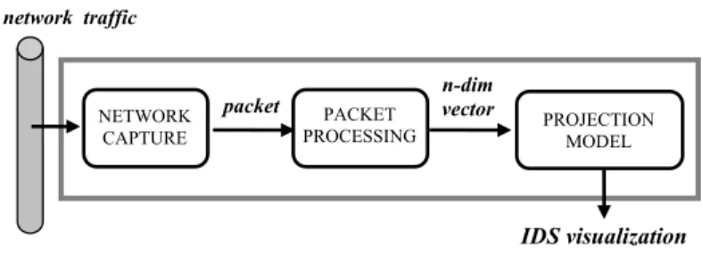
MOVICAB-IDS general architecture.
NETWORK CAPTURE
n-dim vector packet PACKET
PROCESSING PROJECTION MODEL
IDS visualization
network traffic
The general framework for MOVICAB-IDS is depicted in Fig. 1. This framework could be described as follows:
• packets traveling through the network are intercepted by a capture device;
• traffic is coded by a set of features spanning a multidimensional vector space;
• a projection model operates on feature vectors and yields as output a suitable representation of the network traffic. The projection model
clearly is the actual core of the overall IDS. That module is designed to yield an effective and intuitive representation of network traffic, thus
providing a powerful tool for the security staff to visualize network traffic.
To process the continuous flow of network traffic, MOVICAB-IDS split the pre-processed data stream into simple and accumulated
seg-ments as depicted in Fig. 2. These segseg-ments are defined as follows:
− Equal simple segments (Sx): each simple segment contains all the packets with timestamps between the initial and final time limits of the
segment. There must be a time overlap between each pair of consecutive simple segments because anomalous situations could conceivably
take place between simple segment Sx and Sx+1 (where Sx+1 is the next segment following Sx).
− Accumulated segments (Ax): each one of these segments contains several consecutive simple ones. To avoid duplicated packets, time
over-lap is removed in accumulated segments.
One of the main reasons for such a partitioning was to present a long-term picture of the evolution of network traffic to the network
ad-ministrator, as it allows the visualization of attacks lasting longer than the length of a simple segment. To avoid confusion on the part of the
analyst, accumulated segments were visualized at the same time. This prompted the network administrator to realize that there is only one
Fig.
2. MOVICAB-IDS segmentation of pre-processed data.
2.1
Proposed System
Present work focuses on the upgrading of the previously introduced framework, to incorporate new facilities, as described below. The
ini-tial architecture of MOVICAB-IDS is extended to combine clustering methods and projection models, as depicted in Fig. 3.
Fig.
3
.
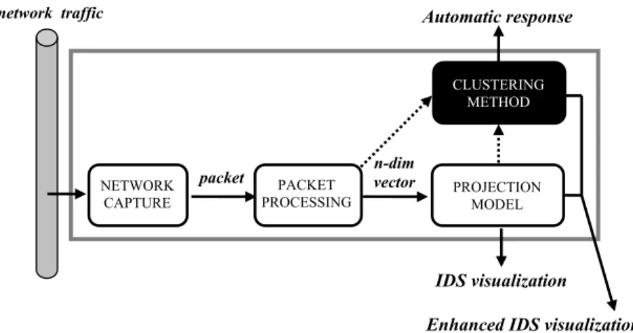
Clustering extension for the proposed system.
NETWORK CAPTURE
n-dim vector packet PACKET
PROCESSING PROJECTION MODEL
IDS visualization
CLUSTERINGMETHOD
Automatic response
Enhanced IDS visualization
network traffic
As automatic response is a desirable feature for an IDS, MOVICAB-IDS is extended in order to do that. For this purpose, human supervision is
not enough so an autonomous way of analysing network traffic is proposed in present work. Clustering methods are proposed and compared in
this study to work in unison with the neural projection model that was previously validated.
The following subsections describe the different techniques that take part in the proposed solution. For the dimensionality reduction as a
projec-tion method, Cooperative Maximum Likelihood Hebbian Learning (Corchado and Fyfe 2003) is explained as it proved to be the most informative
one among many considered (Corchado and Herrero 2011). It is described in section 2.2. On the other hand, to test clustering performance some
of the standard methods have been tested, namely: k-means and agglomerative clustering, described in section 2.3.
PRE-PROCESSED DATA STREAM
t0 t1 t2 t3 t4
S1
S2
S3
S4
A2
A3
A4
Accumulated Segments
Simple Segments
Time
2.2
Cooperative Maximum Likelihood Hebbian Learning
The standard statistical method of Exploratory Projection Pursuit (EPP) (Friedman and Tukey 1974) provides a linear projection of a data set,
but it projects the data onto a set of basis vectors which best reveal the interesting structure in data; interestingness is usually defined in terms
of how far the distribution is from the Gaussian distribution.
One neural implementation of EPP is Maximum Likelihood Hebbian Learning (MLHL) (Corchado et al. 2004), (Fyfe and Corchado
2002). It identifies interestingness by maximising the probability of the residuals under specific probability density functions which are
non-Gaussian.
One extended version of this model is the Cooperative Maximum Likelihood Hebbian Learning (CMLHL) (Corchado and Fyfe 2003)
model. CMLHL is based on MLHL (Corchado et al. 2004), (Fyfe and Corchado 2002) adding lateral connections (Corchado and Fyfe 2003),
(Corchado, Han, and Fyfe 2003) which have been derived from the Rectified Gaussian Distribution (Seung, Socci, and Lee 1998). The
resultant net can find the independent factors of a data set but does so in a way that captures some type of global ordering in the data set.
Considering an N-dimensional input vector (
x
), and an M-dimensional output vector (y
), withW
ijbeing the weight (linking inputj
to output
i
), then CMLHL can be expressed (Corchado and Fyfe 2003), (Corchado, Han, and Fyfe 2003) as:1. Feed-forward step:
Where:
η
is the learning rate,τ
is the "strength" of the lateral connections,b
the bias parameter,p
a parameter related to the energyfunction (Corchado et al. 2004), (Fyfe and Corchado 2002), (Corchado and Fyfe 2003) and
A
a symmetric matrix used to modify theresponse to the data (Corchado and Fyfe 2003). The effect of this matrix is based on the relation between the distances separating the output
neurons.
2.3
Clustering
Cluster analysis (Xu and Wunsch 2009), is the organization of a collection of data items or patterns (usually represented as a vector of
meas-urements, or a point in a multidimensional space) into clusters based on similarity. Hence, patterns within a valid cluster are more similar to
each other than they are to a pattern belonging to a different cluster.
Pattern proximity is usually measured by a distance function defined on pairs of patterns. A variety of distance measures are in use in the
various communities (Andreopoulos et al. 2009), (Zhuang et al. 2012). The clustering output can be hard (allocates each pattern to a single
cluster) or fuzzy (where each pattern has a variable degree of membership in each of the output clusters). A fuzzy clustering can be converted
There are different approaches to clustering data, but given the high number and the strong diversity of the existent clustering methods,
we have focused on the ones shown in Figure 4.
Fig.
4
.
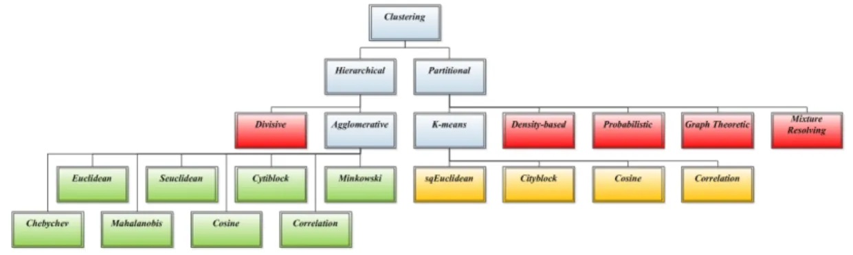
Clustering methods used on this paper: one hierarchical (Agglomerative) and other partitional method (K-means).
At the top level, there is a distinction between hierarchical and partitional approaches. Hierarchical methods produce a nested series of
partitions (illustrated on a dendrogram which is a tree diagram) based on a similarity for merging or splitting clusters, while partitional
methods identify the partition that optimizes (usually locally) a clustering criterion. Hence, obtaining a hierarchy of clusters can provide
more flexibility than other methods. A partition of the data can be obtained from a hierarchy by cutting the tree of clusters at certain level.
Hierarchical methods generally fall into two types:
1. Agglomerative: an agglomerative approach begins with each pattern in a distinct cluster, and successively joins clusters together until a
stopping criterion is satisfied or until a single cluster is formed.
2. Divisive: a divisive method begins with all patterns in a single cluster and performs splitting until a stopping criterion is met or every pattern
is in a different cluster. This method is neither applied nor discussed in this paper.
Partitional clustering aims to directly obtain a single partition of the data instead of a clustering structure, such as the dendrogram
pro-duced by a hierarchical technique. Many of these methods are based on the iterative optimization of a criterion function that reflects the
similarity between a new data and the each of the initial patterns selected for a specific iteration. Partitional methods have advantages in
applications involving large data sets for which the construction of a dendrogram is computationally prohibitive. The problem of these
algorithms is the need of the number of desired output clusters. Exhaustive search over all the set of possible initial labeling for an optimum
output is clearly computationally prohibitive. Therefore, in practice, the algorithm is typically run a number of times with different starting
states, and the best configuration obtained from all of the runs is used as the output clustering. Hence, we can meet different results
depend-ing on the initial labeldepend-ing chosen (usually random). Additional techniques for the groupdepend-ing operation include density-based (Tu et al. 2012),
probabilistic (Brailovsky 1991), graph-theoretic (Argyrou 2009) and mixture-resolving clustering methods, but they are not used on this
paper.
3 Experiments and Results
The main idea behind this experimental study is two-fold: on the one hand it is aimed at discovering whish simple clustering techniques can
be successfully applied to the SNMP intrusion detection problem. On the other hand, it tries to check whether clustering and projection could
work in unison to ease intrusion detection. Additionally, as previously stated, the experimental study tries to show whether clustering could
be more informative applied over the projected data rather than the original data captured from the network. That is, the same data have been
analyzed for intrusion detection, in two different ways, according to what is depicted in Fig. 3. The two considered alternatives are:
This section describes the dataset used for evaluating the proposed clustering methods and how they were generated. The experimental
settings and the obtained results are also detailed.
3.1 Datasets
Five features were extracted from the headers of packets travelling along the network to form the data set:
• Packet ID: sequential integer nonlinear.
• Timestamp: the time difference in relation to the first captured packet. Sequential integer nonlinear.
• Source Port: the port of the source host from where the packet is sent. Discrete integer values.
• Destination Port: the port of the destination host to where the packet is sent. Discrete integer values.
• Size: total packet size (in Bytes).
• Protocol ID: we have used values between 1 and 35 to identify the packet protocol. Discrete integer values.
After initial experiments, it was decided to apply MOVICAB-IDS to the anomalous situations related to SNMP. The Management
Infor-mation Base (MIB) can be defined in broad terms as the database used by SNMP to store inforInfor-mation about the elements that it controls.
Like a dictionary, an MIB defines a textual name for a managed object and explains its meaning.
As previously stated, consideration should be given to SNMP from a security standpoint, due to its very limited security mechanisms and
the security sensitive data that is stored in the MIB. Attackers can exploit these vulnerabilities in the SNMP for network reconnaissance and
remote reconfiguration or shut down of SNMP devices. Thus, MOVICAB-IDS focuses on the most commonly reported types of attacks that
target SNMP:
− SNMP network scan: three types of scans (or sweeps) have been defined: network scans, port scans, and their hybrid block scans (Staniford,
Hoagland, and McAlerney 2002). Unlike other attacks, scans must use a real source IP address, because the results of the scan (open ports or
responding IP addresses) must be returned to the attacker (Ren et al. 2006). A port scan (or sweep) may be defined as series of messages sent
to different port numbers to gain information on its activity status. These messages can be sent by an external agent attempting to access a
host to find out more about the network services that this host is providing. So, a scan is an attempt to count the services running on a machine
(or a set of machines) by probing each port for a response, providing information on where to probe for weaknesses. Thus, scanning generally
precedes any further intrusive activity. This work focuses on the identification of network scans, in which the same port (the SNMP port) is
the target for a number of computers in an IP address range. A network scan is one of the most common techniques used to identify services
that might then be accessed without permission (Abdullah et al. 2005).
− MIB information transfer: this situation involves a transfer of some (or all the) information contained in the SNMP MIB, generally through
the Get command or similar primitives such as GetBulk (Malowidzki 2002; Sprenkels and Martin-Flatin 1999). This kind of transfer is
poten-tially quite a dangerous situation because anybody possessing some free tools, some basic SNMP knowledge and the community string (in
SNMP versions 1 and 2), will be able to access all sorts of interesting and sometimes useful information. As specified by the Internet
Activi-ties Board, the SNMP is used to access MIB objects. Thus, protecting a network from malicious MIB information transfer is crucial.
Howev-er, the "normal" behavior of a network may include queries to the MIB. This is a situation in which visualization-based IDSs are quite useful;
these situations may be visualized as anomalous by an IDS but it is the responsibility of the network administrator to decide whether or not it
constitutes an intrusion.
In addition to the previously mentioned SNMP situations, the analysed datasets contain a great background of network traffic that may be
considered as “normal”. Information about the packets was gathered from a middle-size university network. As used in previous
work contain each one of the anomalous situations on their one, and additionally, another dataset was generated combining both of them.
They can be described as follows:
− Dataset 1: contains three network scans (anomalous situations) that target port numbers 161, 162 and 3750 of all the machines within an IP
address range. The two first ones are the SNMP default port numbers and the third one is introduced as a different case of study.
− Dataset 2: contains "normal" traffic and an MIB information transfer generated by the get-bulk SNMP command.
− Dataset 3: contains three network scans as those in Dataset 1 and an MIB information transfer.
3.2 Details of Applied Clustering Techniques
As similarity is fundamental to the definition of a cluster, a measure of the similarity is essential to most clustering methods and it must
be carefully chosen. Present study applies well-known distance criteria used for examples whose features are all continuous, as described
below.
Table 1.
Some of the well-known distance measures that are usually employed in clustering methods.
Metric
Description
sEuclidean Standardized Euclidean distance. Each coordinate difference between rows in X is scaled by dividing by the corresponding
element of the standard deviation.
Cityblock City block metric also known as Manhattan distance:
∑
Mahalanobis Mahalanobis distance, using the sample covariance of X:
(
)
T(
a b)
b a
ab
x
x
S
x
x
D
=
−
−1−
• xa , xb values of the objects a and b, respectively in the multi-variable space.
• S covariance matrix.
Cosine One minus the cosine of the included angle between points (treated as vectors).
Correlation One minus the sample correlation between points (treated as sequences of values).
The most popular metric for continuous features is the Euclidean distance which is a special case of the Minkowski metric (p=2). It
works well when a data set has compact or isolated clusters (J. Mao 1996). The problem of using directly the Minkowski metrics is the
tendency of the largest-scaled feature to dominate the others. Solutions to this problem include normalization of the continuous features
(sEuclidean distance).
Linear correlation among features can also distort distance measures, it can be relieved by using the squared Mahalanobis distance that
assigns different weights to different features based on their variances and pairwise linear correlations. The regularized Mahalanobis distance
was used in (J. Mao 1996) to extract hyperellipsoidal clusters.
3.2.1
K
-means Algorithm
Four different distance measures are applied in present study for K-means algorithm, as described in Table 2. The proposed solution has
been tested on all of them and the best result can be seen on section 3.3.
Table 2.
Distance measures employed for K-means in this study.
Metric
Description
sqEuclidean Squared Euclidean distance. Each centroid is the mean of the points in that cluster.
Cityblock Sum of absolute differences. Each centroid is the component-wise median of the points in that cluster.
Cosine One minus the cosine of the included angle between points (treated as vectors). Each centroid is the mean of the points in that
cluster, after normalizing those points to unit Euclidean length.
Correlation One minus the sample correlation between points (treated as sequences of values). Each centroid is the component-wise mean
of the points in that cluster, after centering and normalizing those points to zero mean and unit standard deviation.
3.2.2 Agglomerative Clustering
Based on the way the proximity matrix is updated in the second phase, a variety of linking methods can be designed (this study has been
developed with the linking methods shown in Table 3).
Table 3.
Linkage functions employed for agglomerative clustering in this study.
Method Description
Single Shortest distance.
(
,
{
,
}
)
min{
(
,
),
(
,
)}
'
k
i
j
d
k
i
d
k
j
Complete Furthest distance.
(
,
{
,
}
)
max{
(
,
),
(
,
)}
'
k
i
j
d
k
i
d
k
j
d
=
Ward Inner squared distance (minimum variance algorithm), appropriate for Euclidean distances only.
Median Weighted center of mass distance (WPGMC: Weighted Pair Group Method with Centroid Averaging), appropriate for
Euclid-ean distances only.
Average Unweighted average distance (UPGMA: Unweighted Pair Group Method with Arithmetic Averaging).
Centroid Centroid distance (UPGMC: Unweighted Pair Group Method with Centroid Averaging), appropriate for Euclidean distances
only.
Weighted Weighted average distance (WPGMA: Weighted Pair Group Method with Arithmetic Averaging).
Most hierarchical clustering algorithms are based on the single-link and complete-link. These two algorithms differ in the way they
char-acterize the similarity between a pair of clusters:
1. Single-link algorithm: the distance between two clusters is the minimum of the distances between all pairs of patterns drawn from each of the
clusters.
2. Complete-link algorithm: the distance between two clusters is the maximum of all pairwise distances between patterns in each of the clusters.
In either case, two clusters are merged to form a larger cluster based on minimum distance criteria. The complete-link algorithm produces
compact clusters (Baeza-Yates 1992). The single-link algorithm, by contrast, suffers from a chaining effect. It has a tendency to produce
clusters that are straggly or elongated. The clusters obtained by the complete-link algorithm are more compact than those obtained by the
single-link algorithm. The single-link algorithm is more versatile than the complete-link algorithm. However, it has been observed that the
complete-link algorithm produces more useful hierarchies in many applications than the single-link algorithm.
3.3 Results
The best results obtained by applying the previously introduced techniques to the described datasets are shown in this section. The results are
projected through CMLHL and further information about the clustering results is added to the projections, mainly by the glyph metaphor
(colors and symbols). The projections comprise a legend that states the color and symbol used to depict each packet, according to the original
category of the data.
The clustering methods have been applied several times to the analyzed datasets by combining different values for the algorithm options.
The following sections show the best results, whose parameter settings and performance are also detailed. The following subsections
com-prise the results obtained by the projection and clustering technique for each one of the datasets.
Dataset 1
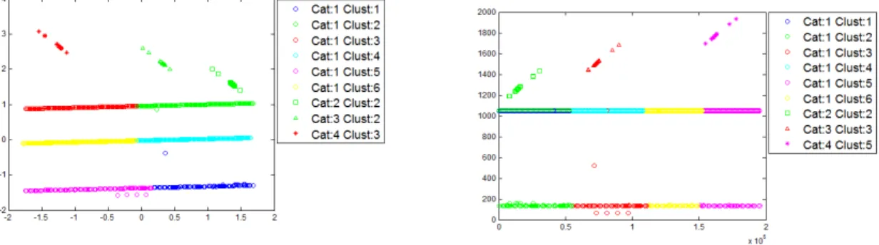
Fig. 5 shows the results obtained by k-means over this dataset. The data has been labeled as follows: normal (Cat. 1), scan to port 161 (Cat.
Fig.
5
.
Best
clustering result under the frame of MOVICAB-IDS through
k
-means for Dataset 1.
5.a
K-means on projected data:
k
=6, sqEuclidean distance.
5.b
K-means on original data:
k
=6, sqEuclidean distance.
From Fig. 5 it can be seen that all the packets from the scans (represented as non-horizontal small bars) are clustered in the same group.
However, some other packets, regarded as normal, have been also included in those clusters. Apart from these two projections, a
comprehen-sive set of experiments has been carried out, whose results can be seen in Table 4. For this experimental study, different values of k
parame-ter were tested; the best of them (in parame-terms of false positive and negative rates) are the ones in the following table.
Table 4. K-means experiments with different conditions for Dataset 1.
Data
k Distance Criteria False Positive False Negative Replicates/
Iterations
Sum of Distances
Projected 2 sqEuclidean 48.0186 % 0 % 5/4 1705.77
Original 2 sqEuclidean 46.6200 % 2.0979 % 5/5 9.75E+11
Projected 4 sqEuclidean 22.9604 % 0 % 5/8 643.352
Original 4 sqEuclidean 69.1143 % 0 % 5/8 4.38E+11
Projected 6 sqEuclidean 22.9604 % 0 % 5/8 301.218
Original 6 sqEuclidean 45.4545 % 0 % 5/24 2.91E+11
Projected 2 Cityblock 46.2704 % 0 % 5/7 1380.1
Original 2 Cityblock 49.6503 % 2.0979 % 5/9 3.50E+07
Projected 4 Cityblock 22.9604 % 0 % 5/8 710.545
Original 4 Cityblock 72.0249 % 0 % 5/15 2.15E+07
Projected 6 Cityblock 22.9604 % 0 % 5/14 526.885
Original 6 Cityblock 48.0187 % 0 % 5/10 1.41E+07
Projected 2 Cosine 47.9021 % 0 % 5/3 316.193
Original 2 Cosine 78.5548 % 0 % 5/5 15.4214
Projected 4 Cosine 22.9604 % 0 % 5/7 86.2315
Original 4 Cosine 46.8531 % 0 % 5/12 3.79324
Projected 6 Cosine 22.9604 % 0 % 5/5 35.9083
Original 6 Cosine 47.2028 % 0 % 5/24 2.51022
Projected 2 Correlation 52.0979 % 0 % 5/3 273.91
Original 2 Correlation 80.0699 % 0 % 5/6 20.6143
Projected 4 Correlation 51.8648 % 0 % 5/7 46.7877
Original 4 Correlation 47.2028 % 0 % 5/16 5.53442
Projected 6 Correlation 27.4876 % 0.3497 % 5/12 16.9416
Original 6 Correlation 47.3193 % 0 % 5/29 3.69279
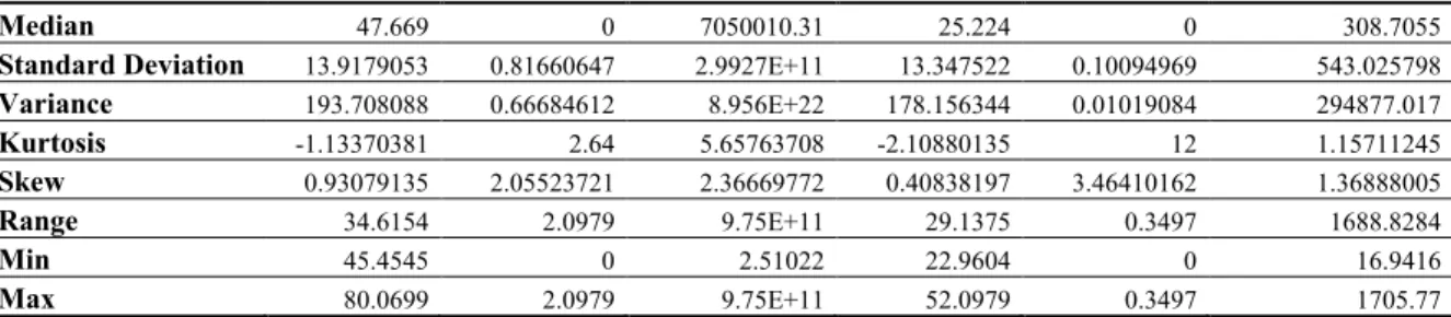
To ease the analysis of the k-means experiments on dataset 1, some statistics have been calculated and are shown in Table 5.
Table 5. Statistics about K-means experiments on Dataset 1.
Original
Projected
False Positive False Negative Sum of Distances False Positive False Negative Sum of Distances
Mean
56.5071167 0.34965 1.4201E+11 34.28365 0.02914167 503.653508Median
47.669 0 7050010.31 25.224 0 308.7055Standard Deviation
13.9179053 0.81660647 2.9927E+11 13.347522 0.10094969 543.025798Variance
193.708088 0.66684612 8.956E+22 178.156344 0.01019084 294877.017Kurtosis
-1.13370381 2.64 5.65763708 -2.10880135 12 1.15711245Skew
0.93079135 2.05523721 2.36669772 0.40838197 3.46410162 1.36888005Range
34.6154 2.0979 9.75E+11 29.1375 0.3497 1688.8284Min
45.4545 0 2.51022 22.9604 0 16.9416Max
80.0699 2.0979 9.75E+11 52.0979 0.3497 1705.77The high false negative rate (FNR) is one of the main problems that most IDS have to face. It can be seen in Tables 4 and 5 that the
pro-posed system achieves an almost zero FNR for dataset 1 in most cases, with very low deviation. For the remaining cases, it keeps as a very
low value as the number of packets in the network scans is much lower than those from normal traffic.
On the other hand, there is not a clear difference (in terms of clustering error) between the experiments on original and projected data,
although for a certain number of clusters, the results on projected data are better. Regarding original and projected data, the false negative
rate is almost similar (0.34965 vs. 0.02914167), being slightly lower in the case of projected data. Additionally, the number of needed
itera-tions is lower for the projected data, as the dimensionality of the data has been previously reduced through CMLHL. By looking at the sum
of distances (sum of point-to-centroid distances, summed over all k clusters), a clear conclusion cannot be drawn as it depends on the
dis-tance method.
Agglomerative clustering has been also applied and the details of the run experiments (with no clustering error) are shown in Table 6.
Two of the best results, with different values for distance criteria, linkage and number of clusters, are depicted in Fig. 5.
Table 6.
Experimental setting of the agglomerative method for Dataset 1.
Data
Distance
Linkage Cutoff
Range
Cluster
Projected Euclidean Single 0.37 0.307 - 0.3803 9 Projected sEuclidean Single 0.37 0.3087 - 0.3824 9 Projected Cityblock Single 0.42 0.4125 - 0.443 9 Projected Minkowski Single 0.38 0.307 - 0.3803 9 Projected Chebychev Single 0.35 0.2902 - 0.366 9 Projected Mahalanobis Single 0.35 0.3084 - 0.3824 9 Original sEuclidean Single 1.80 1.533 - 1.813 5 Original sEuclidean Complete 4.62 4.62 - 4.628 4 Original sEuclidean Average 3.00 2.696 -3.271 4 Original sEuclidean Weighted 3.20 3 - 3.261 4 Original Mahalanobis Single 2.40 2.289 - 2.438 4 Original Mahalanobis Complete 6.00 5.35 - 6.553 3 Original Mahalanobis Average 4.00 3.141 - 4.624 3 Original Mahalanobis Weighted 4.00 3.504 - 4.536 3It can be seen in Table 6 that in the case of projected data, the minimum number of clusters without error is 9, while in the case of
origi-nal data, it could be lowered to 3 with appropriate distance method. From the intrusion detection point of view, a higher number of clusters
does not mean a higher error rate because more than one cluster can be assigned to both normal and attack traffic. In the case of original data,
the sEuclidean and Mahalanobis distances are minimizing the number of clusters without error. On the contrary, some other distance criteria
are applicable for the projected data with same performance regarding clustering error.
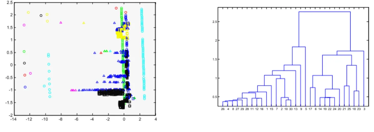
Results from one of the best experiments described in Table 6 are depicted in Fig. 6: traffic visualization and the dendrogram associated
to agglomerative clustering. The following sample has been chosen: Euclidean distance, linkage single, cutoff: 0.37, 9 groups without error.
Fig.
6
.
Best
results of agglomerative
clustering under the frame of MOVICAB-IDS for Dataset 1.
6.a
Agglomerative clustering on projected data.
6.b
Corresponding dendrogram.
Dataset 2
Fig. 7 shows the results obtained by k-means on this data. The data has been labeled as follows: normal (Cat. 1), source-to-destination MIB
transfer (Cat. 2), and destination-to-source MIB transfer (Cat. 3).
Fig.
7
.
Best
clustering result under the frame of MOVICAB-IDS through
k
-means for Dataset 2.
7.a
K-means on projected data:
k
=6, cosine distance.
7.b
K-means on original data:
k
=6, cosine dista
nce.
-14 -12 -10 -8 -6 -4 -2 0 2 4
For the MIB information transfer (dataset 2 in Fig. 7), the clustering does not group data without mistakes as it mixes packets from
dif-ferent categories (two MIB transfer classes and normal traffic). For the original, data, although the number of clusters (k parameter) is the
same, data are more precisely separated. Apart from these two projections, some more experiments have been conducted, whose details
(performance, true positive and false positive rates, values of k parameter, etc.) can be seen in Table 7.
Table 7. K-means experiments with different conditions for Dataset 2.
Data
k Distance Criteria False Positive False Negative Replicates/
Projected 6 Cityblock 3.4400 % 9.5800 % 5/10 3355.85
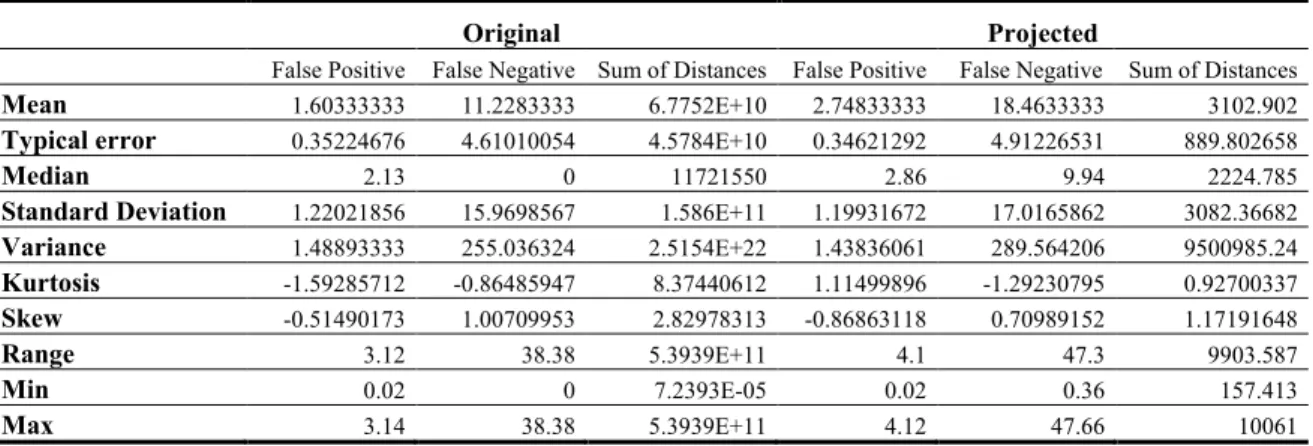
To ease the analysis of the k-means experiments on dataset 2, some statistics have been calculated and are shown in Table 8.
Table 8. Statistics about K-means experiments on Dataset 2.
Original
Projected
False Positive False Negative Sum of Distances False Positive False Negative Sum of Distances
Mean
1.60333333 11.2283333 6.7752E+10 2.74833333 18.4633333 3102.902Typical error
0.35224676 4.61010054 4.5784E+10 0.34621292 4.91226531 889.802658Median
2.13 0 11721550 2.86 9.94 2224.785Standard Deviation
1.22021856 15.9698567 1.586E+11 1.19931672 17.0165862 3082.36682Variance
1.48893333 255.036324 2.5154E+22 1.43836061 289.564206 9500985.24Kurtosis
-1.59285712 -0.86485947 8.37440612 1.11499896 -1.29230795 0.92700337Skew
-0.51490173 1.00709953 2.82978313 -0.86863118 0.70989152 1.17191648Range
3.12 38.38 5.3939E+11 4.1 47.3 9903.587Min
0.02 0 7.2393E-05 0.02 0.36 157.413Max
3.14 38.38 5.3939E+11 4.12 47.66 10061For the MIB transfer, and differentiating from network scans (dataset 1), most experiments got a FNR higher than zero. As can be seen in
table 8, the FNR is once again slightly higher in the case of projected data. For most of those cases, the rates are very low in percentage, and
as the number of packets in the MIB transfer is much higher than those from normal traffic, it means that very few packets of anomalous
traffic are clustered as normal. On the other hand, there is a clear difference (in terms of clustering error) between the experiments on original
and projected data; the results on original data are better in terms or error rates. Additionally, the number of needed iterations is lower for the
projected data, as the dimensionality of the data has been previously reduced through CMLHL. As in previous experiments for dataset 1, the
sum of distances (sum of point-to-centroid distances, summed over all k clusters) does not support a clear conclusion as it strongly depends
on the distance method.
The run experiments for the agglomerative method with very little FPR or no clustering error are shown in Table 9.
Table 9.
Experimental setting of the agglomerative method for Dataset 2.
Original sEuclidean Average 0.8 0 % 40 Original sEuclidean Weighted 1 0 % 34
It can be seen that in the case of projected data, that the minimum number of clusters without error is 25, while in the case of original
da-ta, it could be lowered to 17 with appropriate distance method. In both cases the sEuclidean distance minimizes the number of clusters with
no error. Some other distance criteria are applicable, providing a non-zero value of FPR.
Results from one of the best experiments described in Table 9 are depicted in Fig. 8, including traffic visualization and the associated
dendrogram on projected data. The chosen experiment details are: sEuclidean distance, single linkage, cutoff: 0.4 and 25 groups without
error.
Fig.
8
.
Best
results of agglomerative
clustering under the frame of MOVICAB-IDS for Dataset 2.
8.a
Agglomerative clustering on projected data: sEuclidean,
linkage: single, cutoff: 0.4
8.b
Corresponding dendrogram.
-14 -12 -10 -8 -6 -4 -2 0 2 4 -2
-1.5 -1 -0.5 0 0.5 1 1.5 2 2.5
26 4 8 27 29 28 11 12 16 1 15 7 2 10 30 13 9 5 17 6 14 19 22 24 20 21 25 18 23 3 0.5
1 1.5 2 2.5
Dataset 3
Fig. 9 shows the results obtained by k-means on dataset 3, which includes samples of network scans and MIB information transfer, as it has
been previously described. The data have been labeled as follows: normal (Cat. 1), network scans (Cat. 2), and MIB information transfer
(Cat. 3).
From Fig. 9.b. it can be seen that all the packets in each one of the scans (represented as non-horizontal small bars) are clustered in the same
group. However, some other packets, regarded as normal, have been also included in those clusters. In the selected result, some of the
de-fined clusters do only gather data of one class (rather normal or anomalous traffic) but some other groups do mix traffic from different
clas-ses. Apart from these two projections, some more experiments have been conducted, whose details (performance, true positive and false
Fig.
9
.
Best
clustering result under the frame of MOVICAB-IDS through
k
-means for Dataset 3.
Table 10. K-means experiments with different conditions for Dataset 3.
Data
k Distance Criteria False Positive False Negative Replicates/
Iterations
Sum of Distances
To ease the analysis of the k-means experiments on dataset 3, some statistics have been calculated and are shown in Table 11.
Table 11. Statistics about K-means experiments on Dataset 3.
Original
Projected
False Positive False Negative Sum of Distances False Positive False Negative Sum of Distances
Mean
9.22021667 0.12785833 2.9734E+11 9.843425 0.15343333 1223.00135Typical error
1.15776058 0.07024146 1.84E+11 0.6006213 0.10344473 435.526542tion
Variance
16.0849147 0.05920636 4.0626E+23 4.32895141 0.12840975 2276200.42Kurtosis
0.10714212 1.13010355 5.21076751 7.20243839 2.64 0.55976979Skew
-0.61166909 1.63781177 2.33542803 2.40346377 2.05523721 1.21422466Range
13.1265 0.6137 2.0407E+12 8.5408 0.9206 4569.0197Min
2.165 0 2.06836 7.2963 0 19.4603Max
15.2915 0.6137 2.0407E+12 15.8371 0.9206 4588.48Only few of the experiments on dataset 3 through k-means got a FNR equal to zero. For those cases, a very low value was obtained and,
as the number of anomalous packets is much higher than those from normal traffic, it means that very few anomalous packets are clustered as
normal. On the other hand, as can be seen in table 11, there is not a clear difference (in terms of clustering error) between the experiments on
original and projected data, although for a certain number of clusters, the results on projected data are better. Additionally, the number of
needed iterations is lower for the projected data, as the dimensionality of the data is lower. By looking at the sum of distances (sum of
point-to-centroid distances, summed over all k clusters), a clear conclusion cannot be drawn as it depends on the distance method.
Comprehensive details of the run experiments with very little FPR or no clustering error are shown in Table 12, for the case of
agglomer-ative clustering.
Table 12.
Experimental setting of the agglomerative method for Dataset 3.
Data
Distance
Linkage Cutoff False Positive Cluster
Projected Euclidean Single 0.15 0.1363 % 31 Projected sEuclidean Single 0.15 0.1363 % 31 Projected Cityblock Single 0.2 0.2216 % 28 Projected Minkowski p=3 Single 0.15 0.1534 % 26 Projected Chebychev Single 0.12 0.1363 % 32 Projected Mahalanobis Single 0.16 0.1363 % 29 Original sEuclidean Single 0.4 0 % 33 Original Cityblock Single 1200 0 % 58 Original Mahalanobis Single 0.6 0 % 32From Table 12 we can conclude that in the case of projected data, a non-error clustering is not obtained by agglomerative method, but the
FPR can be greatly reduced. To do so, around 30 clusters are obtained, depending on the clustering method. In the case of original data, 33 is
the minimum number of clusters without error choosing the appropriate distance method. In both cases, the sEuclidean distance minimizes
the number of clusters.
The results depicted on Fig. 10 (traffic visualization and the associated dendrogram to agglomerative clustering) are associated to the
Fig.
10
.
Best
results of agglomerative
clustering under the frame of MOVICAB-IDS for Dataset 3.
10.a
Agglomerative clustering on projected data:
sEuclide-an, linkage: single, cutoff: 0.15.
10.b
Corresponding dendrogram.
-3 -2 -1 0 1 2 3 4 5
This paper has proposed the use of clustering techniques to perform ID on numerical traffic data sets in unison with neural projection
tech-niques. Simple clustering methods have been applied to SNMP anomalous situations to get an idea about the performance of the proposal.
Detailed conclusions about experiments on the different datasets and with several different clustering techniques and criteria, can be found in
section 3. The studied SNMP-related anomalous situations (network scans and MIB information transfers) have been both independently and
jointly analyzed. Experimental results show that some of the applied clustering methods, mainly hierarchical ones, obtain a good clustering
performance on the analysed data, according to false positive and negative rates. The obtained results vary from the different analysed
da-tasets and the behaviour of the applied clustering techniques is not always the same.
In general terms, it can be said that the performance of the clustering techniques varies between the two different SNMP anomalous
situa-tions. Regarding the distance criteria, none of them is clearly the best one, so its selection will depend on the analysed data. Finally, by
considering projected versus original data, it can be said that the latter obtained higher FNR, but one of its main advantages is the smaller
execution time, what is not covered in present work.
Finally, it can be concluded that the applied methods are able to properly detect anomalous situations when projected together with normal
traffic. It has been proven that clustering methods could help in intrusion detection not only by applying them to the same data that is
pro-jected but in a subsequent way.
Acknowledgments
This research is partially supported through projects of the Spanish Ministry of Economy and Competitiveness with ref:
TIN2010-21272-C02-01 (funded by the European Regional Development Fund), and SA405A12-2 from Junta de Castilla y León.
References
Abdullah, K., C. Lee, G. Conti, and J. A. Copeland. 2005. Visualizing Network Data for Intrusion Detection. Paper read at Sixth Annual
IEEE Information Assurance Workshop - Systems, Man and Cybernetics.
Andreopoulos, Bill, Aijun An, Xiaogang Wang, and Michael Schroeder. 2009. A roadmap of clustering algorithms: finding a match for a
Argyrou, A. 2009. Clustering Hierarchical Data Using Organizing Map: A Graph-Theoretical Approach. In Advances in
Self-Organizing Maps, Proceedings, edited by J. C. Principe and R. Miikkulainen. Berlin: Springer-Verlag Berlin.
Baeza-Yates, R. A. 1992. Introduction to data structures and algorithms related to information retrieval. Information Retrieval: Data
Struc-tures and Algorithms, W. B. Frakes and R. Baeza.Yates, Eds. Prentice-Hall, Inc., Upper Saddle River, NJ.:13-27.
Brailovsky, V.L. 1991. A probabilistic approach to clustring. Pattern Recognition. Lett. 12, 4:193-198.
Bratman, M.E. 1987. Intentions, Plans and Practical Reason: Harvard University Press, Cambridge, M.A.
Carrascosa, C., J. Bajo, V. Julián, J.M. Corchado, and V. Botti. 2008. Hybrid Multi-agent Architecture as a Real-Time Problem-Solving
Model. Expert Systems with Applications: An International Journal 34 (1):2-17.
Case, J., M.S. Fedor, M.L. Schoffstall, and C. Davin. 1990. Simple Network Management Protocol (SNMP). In IETF RFC 1157.
Case, J., K. McCloghrie, M. Rose, and S. Waldbusse. 1993. Introduction to Version 2 of the Internet-standard Network Management
Frame-work. In IETF RFC 1441.
Corchado, E., J. M. Corchado, L. Saiz, and A. Lara. 2004. Constructing a Global and Integral Model of Business Management Using a CBR
System. Paper read at CDVE 2004.
Corchado, E., and C. Fyfe. 2003. Connectionist Techniques for the Identification and Suppression of Interfering Underlying Factors.
Interna-tional Journal of Pattern Recognition and Artificial Intelligence 17 (8):1447-1466.
Corchado, E., Y. Han, and C. Fyfe. 2003. Structuring Global Responses of Local Filters Using Lateral Connections. Journal of Experimental
& Theoretical Artificial Intelligence 15 (4):473-487.
Corchado, Emilio, and Álvaro Herrero. 2011. Neural Visualization of Network Traffic Data for Intrusion Detection. Applied Soft Computing
11 (2):2042–2056.
Cui, K. Y., and Ieee. 2012. Research On Clustering Technique In Network Intrusion Detection, 2012 International Conference on Industrial
Control and Electronics Engineering. Los Alamitos: Ieee Computer Soc.
Davin, J., J. Galvin, and K. McCloghrie. 1992. SNMP Administrative Model. In IETF RFC 1351.
Di Pietro, Roberto, and Luigi V. Mancini. 2008. Intrusion Detection Systems. Vol. 38, Advances in Information Security: Springer.
Friedman, J. H., and J. W. Tukey. 1974. A Projection Pursuit Algorithm for Exploratory Data-Analysis. IEEE Transactions on Computers 23
(9):881-890.
Fyfe, C., and E. Corchado. 2002. Maximum Likelihood Hebbian Rules. Paper read at 10th European Symposium on Artificial Neural
Net-works (ESANN 2002).
Ge, L., and C. Q. Zhang. 2012. The Application of Clustering Algorithm in Intrusion Detection System. In Advances in Future Computer and
Control Systems, Vol 1, edited by D. Jin and S. Lin. Berlin: Springer-Verlag Berlin.
Herrero, Álvaro, and Emilio Corchado. 2009. Mining Network Traffic Data for Attacks through MOVICAB-IDS. In Foundations of
Compu-tational Intelligence: Springer.
Herrero, Álvaro, Emilio Corchado, Paolo Gastaldo, and Rodolfo Zunino. 2009. Neural Projection Techniques for the Visual Inspection of
Network Traffic. Neurocomputing 72 (16-18):3649-3658.
Herrero, Álvaro, Emilio Corchado, María A. Pellicer, and Ajith Abraham. 2009. MOVIH-IDS: A Mobile-Visualization Hybrid Intrusion
Detection System. Neurocomputing 72 (13-15):2775-2784.
J. Mao, A.K. Jain. 1996. A self-organizing network for hyperellipsoidal clustering (HEC). IEEE Trans. Neural Netw. 7:16-29.
Jiang, ShengYi, Xiaoyu Song, Hui Wang, Jian-Jun Han, and Qing-Hua Li. 2006. A Clustering-based Method for Unsupervised Intrusion
Malowidzki, Marek. 2002. GetBulk Worth Fixing. The Simple Times 10 (1):3-6.
Myerson, J.M. . 2002. Identifying Enterprise Network Vulnerabilities. International Journal of Network Management 12 (3):135-144.
Northcutt, S., M. Cooper, K. Fredericks, M. Fearnow, and J. Riley. 2001. Intrusion Signatures and Analysis: New Riders Publishing
Thou-sand Oaks,.
Qiao, L. B., B. F. Zhang, Z. Q. Lai, J. S. Su, and Ieee. 2012. Mining of Attack Models in IDS Alerts from Network Backbone by a Two-stage
Clustering Method. In 2012 Ieee 26th International Parallel and Distributed Processing Symposium Workshops & Phd Forum.
New York: Ieee.
Ren, P., Y. Gao, Z. C. Li, Y. Chen, and B. Watson. 2006. IDGraphs: Intrusion Detection and Analysis Using Stream Compositing. IEEE
Computer Graphics and Applications 26 (2):28-39.
Seung, H. S., N. D. Socci, and D. Lee. 1998. The Rectified Gaussian Distribution. Advances in Neural Information Processing Systems
10:350-356.
Sprenkels, Ron, and Jean Philippe Martin-Flatin. 1999. Bulk Transfers of MIB Data. In Technical Report SSC/1999/009: Communication
Systems Division. Swiss Federal Institute of Technology Lausanne.
Staniford, Stuart, James A. Hoagland, and Joseph M. McAlerney. 2002. Practical Automated Detection of Stealthy Portscans. Journal of
Computer Security 10 (1-2):105-136.
The Top 10 Most Critical Internet Security Threats (2000-2001 Archive). 2001. SANS Institute.
Tu, Q., J. F. Lu, B. Yuan, J. B. Tang, and J. Y. Yang. 2012. Density-based hierarchical clustering for streaming data. Pattern Recognition
Letters 33 (5):641-645.
Vulnerability Statistics Report. 2000. Cisco Secure Consulting.
Xu, R., and D.C. Wunsch. 2009. Clustering: Wiley.
Zheng, Q. H., Y. G. Xuan, and W. H. Hu. 2011. An IDS Alert Aggregation Method Based on Clustering. In Advanced Research on
Infor-mation Science, AutoInfor-mation and Material System, Pts 1-6, edited by H. Zhang, G. Shen and D. Jin. Stafa-Zurich: Trans Tech
Publications Ltd.
Zhuang, W. W., Y. F. Ye, Y. Chen, and T. Li. 2012. Ensemble Clustering for Internet Security Applications. Ieee Transactions on Systems