TítuloSpectral Heart Rate Variability analysis using the heart timing signal for the screening of the Sleep Apnea–Hypopnea Syndrome

Spectral Heart Rate Variability analysis using the heart timing signal

for the screening of the Sleep Apnea

–

Hypopnea Syndrome

Diego Alvarez-Estevez

, Vicente Moret-Bonillo

Sleep Centre, Medisch Centrum Haaglanden and Bronovo-Nebo, The Hague, The Netherlands

b_{Laboratory for Research and Development of Artificial Intelligence, University of A Coruña, A Coruña, Spain}

a r t i c l e i n f o

Article history:

Received 29 November 2015 Received in revised form 6 January 2016 Accepted 22 January 2016

Keywords:

Heart Rate Variability Heart timing signal IPFM model Spectral analysis

Sleep Apnea–Hypopnea Syndrome

a b s t r a c t

Some approaches have been published in the past using Heart Rate Variability (HRV) spectral features for the screening of Sleep Apnea–Hypopnea Syndrome (SAHS) patients. However there is a big variability among these methods regarding the selection of the source signal and the specific spectral components relevant to the analysis. In this study we investigate the use of the Heart Timing (HT) as the source signal in comparison to the classical approaches of Heart Rate (HR) and Heart Period (HP). This signal has the theoretical advantage of being optimal under the Integral Pulse Frequency Modulation (IPFM) model assumption. Only spectral bands defined as standard for the study of HRV are considered, and for each method the so-called LF/HF and VLFnfeatures are derived. A comparative statistical analysis between the different resulting methods is performed, and subject classification is investigated by means of ROC analysis and a Naïve-Bayes classifier. The standard Apnea-ECG database is used for validation purposes. Our results show statistical differences between SAHS patients and controls for all the derived features. In the subject classification task the best performance in the testing set was obtained using the LF/HF ratio derived from the HR signal (Area under ROC curve¼0.88). Onlyslight differences are obtained due to the effect of changing the source signal. The impact of using the HT signal in this domain is therefore limited, and has not shown relevant differences with respect to the use of the classical approaches of HR or HP.

&2016 Elsevier Ltd. All rights reserved.

1. Introduction

The Sleep Apnea_–Hypopnea Syndrome (SAHS) is a common disorder characterized by the repeated occurrence of involuntary breathing cessations during sleep. Studies carried out during the last years have estimated the prevalence of SAHS to range between 4% and 6% in the average adult population. Lack of treatment is associated with excessive daytime sleepiness, fatigue, develop-ment of cardiovascular diseases, hypertension, or brain damage

[1]. The standard diagnostic procedure requires of a polysomno-graphic (PSG) study to be carried out in which the physiological activity of the patient is monitored during the night. The analysis of the PSG data, however, requires a lot of effort from the clinician and is expensive, especially when carried out in-hospital attended conditions. Therefore automatic diagnosis of SAHS has become an important area of interest. Specially, there is a growing interest in the recent years towardfinding quicker screening procedures that also allow ambulatory patient monitoring. These procedures

would help reducing the current long waiting lists for clinical PSG examinations, the associated diagnostic costs, and would allow for better patient scheduling and prioritization.

The work published in 1984 by Guilleminault et al. stated for thefirst time the characteristic cyclical variation of the heart rate in sleep apnea patients. In this work it was observed that at the beginning of an apneic event the subject would suffer from pro-gressive bradycardia followed by a period of tachycardia while the breathing resumes. It was concluded that the changes observed in SAHS were caused as a consequence of the autonomic nervous system mediation. In the same paper it was suggested that this cyclical variation of the heart rate could by detected by computer analysis and used as a screening tool for SAHS [2]. Such a hypothesis motivated further research on whether the respiratory information contained in the electrocardiogram (ECG) could be used for the detection of apneic events, both in the clinical and in the engineering domain[3,4]. In this regard, it is our interest in this paper to focus over the so-called spectral methods for the analysis of the Heart Rate Variability (HRV).

Standards of measurement and interpretation of the HRV at this respect decompose the frequency spectrum in a series of spectral components of clinical interest. Specifically the High Contents lists available atScienceDirect

journal homepage:www.elsevier.com/locate/cbm

Computers in Biology and Medicine

http://dx.doi.org/10.1016/j.compbiomed.2016.01.023 0010-4825/&2016 Elsevier Ltd. All rights reserved.

n_{Corresponding author.}

Frequency band (HF, 0.15–0.4 Hz) is related to the parasympathetic regulatory component of the heart rate, whereas the Low Fre-quency component (LF, 0.04–0.15 Hz) can reflect both sympathetic and parasympathetic modulation. It is generally accepted, how-ever, that when LF is expressed in normalized units, the sympa-thetic regulatory component is reinforced[4,5]. The LF/HF ratio, as a consequence, was traditionally considered by many to be an indicator of the sympatho-vagal balance that regulates the heart rate[5]. This interpretation however is nowadays questioned, and therefore, although commonly reported and potentially mean-ingful, outcomes of the LF/HF ratio have to be interpreted with caution [4]. Finally, the Very Low Frequency component (VLF, 0.003–0.04 Hz) although still controversial, it is generally asso-ciated with various slow mechanisms of the parasympathetic function, and it has been shown to be increased during sleep-disordered breathing[4,6,7].

When applied to SAHS, several works have been published in the past that explored statistical differences in the standard HRV spectral components between patients and controls [6,8–13]or between apneic periods and normal breathing [14–18]. Among these works some have found the LF/HF to be a relevant dis-criminating feature, whereas some other have reported more important differences in the range of the VLF band[6,12,13,18]. Literature is however controversial with some studies condition-ing significance only to certain severity groups[8,10,11]or even ruling it out[17].

The use of spectral HRV features to differentiate patients from controls in the SAHS domain can also be found in several works throughout the literature [19–24]. Nevertheless no standard method has been established and therefore there is a big varia-bility regarding, for instance, the series of data subject to spectral analysis, the power spectral estimation method, the handling of artifacts or the specific spectral components relevant to the ana-lysis [23–25]. Variability in the methodology and the lack of standardization makes somewhat difficult to make comparisons in order to derive meaningful medical interpretations. The use of mathematical physiological models and clinical standard guide-lines would be preferable to overcome this issue.

The integral pulse frequency modulation (IPFM) model has been assumed for many authors to explain the mechanisms of the autonomic regulation of the heart rate [26–28]. This model assumes a modulating signal which influences the sino-atrial node generating the beat occurrences. Classical spectral analysis meth-ods of the HRV, actually, implicitly assume the existence of such a modulating signal whose spectral properties are usually estimated through the use of subrogate signal sources like the Heart Rate (HR), the Heart Period (HP), the tachogram, or the spectrum of counts [5]. Mateo and Laguna [25] have shown that these approximations introduce a certain distortion in the spectrum as compared to the expected spectral information carried by the modulating signal according to the IPFM model. In the same work, on the other hand, they introduce the new Heart Timing (HT) signal, which is optimal in the same IPFM sense (i.e. the difference with the expected spectrum is minimal as compared with the above mentioned approaches)[26].

Given this context, it is our aim to test the usefulness of the HT signal in the discrimination of healthy controls and patients affected by SAHS. Specifically we make a comparison between the LF/HF ratios and the so-called VLFn indices obtained from this signal, and those derived from the HR and the HP signals using different spectral estimation methods. For this purpose we follow the standard HRV spectral band definitions as recommended in the clinical guidelines [5]. Finally we test the different HRV-derived features to classify individuals of the two populations using a public standard database[29]investigating their useful-ness in the screening of SAHS. To our knowledge, this is thefirst

work investigating the use of the HT signal in thefield of SAHS diagnostics. Even more, that we know of this is also thefirst time that the HT signal is applied to discriminate patho-physiological states in a practical domain.

2. Materials and methods

2.1. The Apnea-ECG database

The Apnea-ECG database is used for validation purposes in this study. This database was created as part of a competition orga-nized in the context of the Computers in Cardiology (CinC) 2000 conference[30]. The aim was to study the viability of using the respiratory information contained in the ECG for the diagnosis of SAHS. Originally the Apnea-ECG database was composed of a total of 70 recordings, divided into two sets (training and test) of 35 recordings each[29]. Expert’s annotations on apnea and hypopnea events are available on a minute-by-minute basis for each recording, which are further classified into three subgroups on the basis of the amount of minutes containing apneic events: group A (100 min or more), group B (between 5 and 99 min), and group C (less than 5 min). A total of 20, 5 and 10 recordings, both in the training and in the testing sets, are respectively classified in the three groups. A sleep standard single-lead derivation was used to record the ECG which was sampled at 100 Hz.[29].

Since its publication, the Apnea-ECG database has become very popular and it has been used as standard benchmark by many researches to compare the performance of different ECG-based algorithms in the scoring of sleep apnea.[3,20–24,31–33].

For our study, we take the recordings belonging to the sub-group A in Apnea-ECG as representative of Obstructive Sleep Apnea (OSA) patients (OSA group), while the recordings within the C subgroup are used as the control group. The mild severity group corresponding to category B in the Apnea-ECG database is not used here. Resulting data are summarized inTable 1in which the corresponding SAHS severity per recording is characterized using the standard Apnea–Hypopnea Index (AHI) which determines the number of apneas and hypopneas per hour of sleep.

2.2. The IPFM model and the HT signal

The Integral Pulse Frequency Modulation (IPFM) model explains the generation of beat occurrences based on the hypothesis that the sympathetic and parasympathetic influences on the sino-atrial (SA) node can be represented by a single mod-ulation signal m(t). This input signal m(t) is integrated until a certain threshold,R, is reached. The former can be viewed as the charging process of the sino-atrial membrane potential. When the threshold of the membrane is reached, the system triggers an action potential that materializes in the generation of a beat. At this point the integrator is reset to zero, and a new cardiac cycle begins[28].

Table 1

Data used in the study extracted from the Apnea-ECG database. Data is shown as mean and standard deviation (in parentheses); n¼number of recordings; TR¼Training Dataset; TS¼Testing Dataset; OSA¼Obstructive Sleep Apnea; AHI¼Apnea–Hypopnea Index.

OSA group Control group

n AHI n AHI

TR 20 47.66 (20.14) 10 0.03 (0.08)

We can represent the operation of the IPFM model through the

wherek is an integer number representing thek-th beat and tk reflects its time stamp. The timeTis the mean interbeat interval and (1þm(t))/Tcan be seen as the instantaneous heart rate. Them (t)/Tpart in (1) represents the zero-mean modulating term, which is presumed to be small (m(t)_{1) re_flecting that Heart Rate Variability is usually smaller than the mean heart rate. Also in general, it is considered thatm(t)is band-limited with negligible power for frequencies above 0.4 Hz.

In Mateo and Laguna [25] the authors introduced the gen-eralization of the IPFM model to the continuous time by which(1)

can be rewritten as

where t(x)is a continuous function that solves the IPFM model equation, and whose samples atx¼k¼1,2,…,naret(k)¼tk. Using the generalization given in(2), thecontinuous heart timing signal,

ht(t)or HT, is defined as follows[25]:

ht tð Þ ¼x tð ÞTt¼ Z t

0

mð Þ

τ

τ

Indeed, according to(3), the continuous HT signal can be sim-ply defined as the integral ofm(t). Also from(3)derives that the relationship betweenht(t)and HRV is straightforward, beinght(t) also linearly related tom(t).

In the frequency domain, taking into account thatm(t)is causal and with zero-mean, the following equation holds:

HT wð Þ ¼MðwÞ

jw ð4Þ

whereHT(w)andM(w)are, respectively, the Fourier transforms of

ht(t)and m(t). In other words, if we know ht(t)or its regularly

spaced samples satisfying the Nyquist criterion, the spectrum ofm (t),M(w), can be exactly determined[25].

2.3. Spectral HRV analysis using the HT signal

In 1981, Akselrod et al. introduced power spectral analysis of heart ratefluctuations as a tool to quantitatively evaluate beat-to-beat cardiovascular control[34]. Methods for the spectral analysis of the HRV look for differences in the spectral components of HRV-related signals, which are usually defined in the time domain based on the processing of the ECG beat sequence. In the litera-ture, several sources signals can be found on this regard subject to spectral analysis [5,25]. Among them, the HR and the HP have been widely used which can be defined as:

hr tð Þ ¼k it actually can be simply defined as the inverse of HP, thus in beats per second. The former is though more extended and thus it will be preferred. Both, the HR and the HP signals are used in this work for comparison purposes.

The term“Heart Rate Variability”, indeed, is arbitrarily accepted to refer to the variations produced in the interval between con-secutive heart beats as well as the oscillation between concon-secutive instantaneous heart rates[5]. In this sense, HR and HP are intui-tively related to HRV, and even though empirical results have shown the usefulness of these two signals when analyzing HRV

[5], there is still the lack of a mathematical model that allows a complete characterization of such relationship.

The use of the HT signal, on the other hand, allows making predictions and interpretations in the context of the IPFM model. HRV analysis in this sense implies in practice obtaining as much information as possible about the modulating signalm(t)using the sequence of observed beats. At this respect, and using (3) the unevenly spaced samples of the HT signal can be derived at the beat timestkas[25]:

ht tð Þ ¼k kTtk¼ Z tk

0

mð Þ

τ

τ

The fact that signals (5)–(7), and whichever signal generated from the beat sequence, are unevenly spaced, matters, and espe-cially if the objective is to analyze HRV in the spectral domain. At this purpose several methods have been proposed in the literature to overcome this problem, namely assuming that HRV signals are evenly sampled, using direct spectral estimation methods (e.g. Lomb) and by using interpolation methods to generate an evenly sampled version from the irregularly sampled input. At this respect it has been shown in[25], that when the IPFM model is assumed, an appropriate interpolation method with adequate frequency response is the option that best preserves the mod-ulation properties of the m(t) signal. Specifically, it has been shown that the method that produces the best spectrum estimates is obtained when the Fourier Transform (FT) of the HT series interpolated by high order splines is used.

Indeed, once the regularly spaced samples HT series is obtained, the spectrum of the IPFM modulating signalm(t),M(w), which is the focus of our interest, can be directly retrieved as stated in the previous section by using(4).

2.4. Artifact removal

The quality of the QRS detector output is compromised by the presence of artifacts and the occurrence of ectopic beats. Thefirst can produce false positives or false negatives in the beat sequence that will affect both the morphology and the spectral properties of the derived HRV signals. Artifacts due to the presence of ectopic beats on the other hand, can generally be classi_fied in ventricular or supraventricular depending on the ectopic focus. Ectopic beats with a ventricular origin do not reset the normal activity of the SA node. Usually the normal beat would be replaced by a morpho-logically different ectopic beat. Supraventricular ectopic beats, however, have a similar morphology to normal beats, but reset the SA node activity.

These abnormalities are frequent and considerably compromise the reliability of the of the derived HRV signals, and therefore of their corresponding spectral estimates. To avoid this problem in the framework of the IPFM model, Mateo and Laguna[35]have proposed a method based on the fact that, under this model, the variation produced in the instantaneous heart rater(t)due to the presence of normal beats is band limited.

Hence, using this assumption, it is possible to impose a thresholdUon the derivative of the instantaneous heart rater0(t) to enable the acceptance of a beat as belonging to the normal SA sequence. This condition can be implemented using the following equation[35]:

Computation of HT in the presence of ectopic beats should not be performed directly by using(7). Indeed, the estimated mean heart periodTwould be affected by the ectopic gap and the HT values in the neighborhood of an ectopic beat would be largely mistaken due to the regular concordance lost between the integer kand the beat positiontk. Instead, the proposed solution involves the extension of the IPFM model to include the resetting of the SA node in the presence of ectopic beats. In this respect, given a series of heart beats with an ectopic beat detected at thekeposition,(7)

can be rewritten as follows to compute the correct values of HT for the beats preceding and following the ectopic occurrence:

ht tð Þ ¼k

wheresis an unknown real quantify (sr1) corresponding to the value reached for the integral in (2) at the resetting time t (ke1þs), and T is the actual mean heart period. These two a priori unknownsandTvalues can be estimated (see[35],Section II.B), after which(9)can be used to obtain the HT series at the irregularly spaced beat times tk. Finally, by using spline inter-polation, the continuous estimate of the HT signal can be derived and the spectrum ofm(t)can be obtained according to(4).

3. Experimental procedures

The following sections describe the processing steps followed to derive the features of LF/HF and VLFnfrom the source signals of HR, HP and HT, and using different spectral estimation methods. The Apnea-ECG database is used as benchmark as described in

Section 2.1. We are interested in studying the differences between the obtained indices and evaluate their usefulness to perform subject classification for the screening of SAHS.

3.1. ECG features extraction

For each recording QRS detection is performed over the ECG using an algorithm based onfilter banks as proposed in Alfonso et al.[36]. Fiducial points corresponding to the R peaks are used as thetkpoints,k¼0..nqrs-1, wheret0is the time occurrence of the first detected beat. From thetkseries the unevenly spaced samples of HR and HP are straightforward obtained respectively according to(5)and(6). The samefiducial points are used to compute the unevenly spaced samples of HT according to(7), whereTis taken as the mean interbeat interval,T¼tnqrs1t0

nqrs1 .

3.2. Artifact processing

As explained inSection 2.4false QRS detections (FP or FN) and ectopic beats would seriously affect both time and spectral prop-erties of the derived HRV signals. To solve this problem and get rid of these anomalies, the detection method described inSection 2.4

is applied in order to identify and classify the artifacts in the beat series, which are then removed from the sequence of normal beats. Detection threshold U¼min 0:5;4:3

σ

is applied in(8), where the upper limit U¼0.5 s2 is imposed to reject possible episodes of atrialfibrillation or other arrhythmias.

It is worth to mention that for stability of the artifact classifi -cation process subsequent to(8)(see[35],Section II.Afor details) and of posterior interpolation processes (described here next in

Section 3.3), we have found useful to impose the requirement that thefirst 10 samples of jrb0_kj must be considered artifact-free (i.e.

jr0_kd_¼1::10joU). That means that until this condition is not satisfied, all the preceding beats will be automatically discarded from the sequence of normal beats and will be no longer considered.

As the output of this process, we get the beat series where each beat has been classified either as normal (N), as FN, as FP, or as ectopic. The resulting sequence containing only N beats is used to recalculate the HR and the HP series by using(5)and(6). In this case, however, only sequences derived from normal-to-normal (NN) intervals are admitted and concatenated. For HT, as explained inSection 2.4, the series needs to be recomputed. For this purpose and using only the sequence of normal and ectopic beats (detected FNs and FPs are removed from the list) Eq.(9)is applied using the ectopic occurrences as thekepoints, where for each one, the corresponding estimate of the jumpsis calculated, as well as the resulting mean heart periodT(see

[35],Section II.Bfor details). A new unevenly spaced series of HT is obtained as a result, where the effects due to the presence of artifacts and ectopic beats have been corrected.

3.3. Signal interpolation

Spline interpolation is used on the previous irregularly spaced series of HR, HP and HT to obtain the corresponding evenly sam-pled signals for the purpose of performing subsequent spectral analysis. In [25,35]it has been shown that signal interpolation with high order splines followed by Discrete Fourier Transform (DFT) provides the best spectrum estimates of the sino-atrial node modulation signal. Comparison includes most of the state-of-the-art methods such as the spectrum of counts, linear interpolation, the Berger’s method, parametric autoregressive estimation, or direct estimation methods such as the Lomb spectrum.

In our case we use spline interpolation both of order three“cubic”

and fourteenth, as suggested in[25]and for comparison purposes. We use an output interpolation frequency of 4 Hz. Specifically it is our interest to see whether the theoretical improvement achieved by the use of high-order splines may influence the derived HRV features extracted from the resulting spectra (in our case, the LF/HF ratio and the VLFnindex).

We have imposed a limit to the interpolation gap of UintGap¼2 s. Indeed, spline interpolation of a sequence (HR, HP or HT) when the time gap is bigger than 5 s would produce a result that could be regarded as purely speculative. Thus sequences where the interpolation gap is greater thanUintGapare discarded and do not contribute to the subsequent spectral estimation.

3.4. Spectral estimation

DFT-based power spectral density (PSD) of the interpolated series is estimated using two different variants: (i) regular periodogram estimation using the Fast Fourier Transform (FFT) applied to the full (artifact-free) series, and (ii) using a modified version of the Welch method. In any case (full or Welch) a Hamming window is used and zero-padding is applied to reach the next power of 2 that resulted from eachN-length input segment. In the case of (i), we takeNas the maximum length amongst all the recordings since zero-padding does not modify the resulting spectra. For (ii) default window size of 5 min is used as recommended by HRV analysis standards[5]with a 50% window overlap at each step. This results in a resolution of at least 0.003 Hz per bin in each window, but note than in (i) this resolution is normally much higher. DC component removal is performed in either case (full or Welch) by subtracting the mean value from the corre-sponding input segment before the FFT application.

performed in the basis of 5-min windows, and therefore we remove (skip) from the Welch calculation those windows over-lapping sequences affected by such interpolation gaps.

Finally, note that in the case of HT, before the spectral trans-formation, we apply (3) from which is derived thatm(t)¼ht0(t). In fact we are interested in studying the spectral properties ofm(t), rather than ht(t), thus in the case of HT, the interpolated m(k) series is actually used as the input for the FFT. This is equivalent to apply(4)in order to obtainM(w).

As a result of the above described process, we obtain two different spectral estimators for each evenly-spaced HRV derived signals (i.e. HR, HP or HT), respectively for (i) using the regular periodogram, and for (ii) using the Welch spectrum. The following notation will be used: HRP, HPP, HTPin the case of (i), and HRw, HPw, HTwrespectively in the case of (ii). In addition for each of these estimates two versions are obtained dependent upon the order of the interpolating splines. In this case, when relevant, the corresponding order of the splines will be specified at the end of the notation: for instance,HRw3, to refer to the spectrum obtained from the HR signal interpolated with cubic splines, and using with the Welch method. Likewise, HTP14 will refer to the

spectrum obtained from the HT signal interpolated with 14th order splines, and using the periodogram, and so on.

Over the resulting spectra, power in relevant frequency bands (VLF, LF and HF) is extracted according to standard HRV rules[5]

and the LF/HF is calculated for each spectrum estimate. In addition the VLFnindex feature is computed as follows:

VLFn¼

P

0:04

Hz¼0:003

PSDðwÞ

P

0:4

Hz¼0

PSDðwÞ 0P:003

Hz¼0

PSDðwÞ

ð10Þ

thus representing the power in the VLF spectral band normalized to the total power minus the power in the ULF band[5].

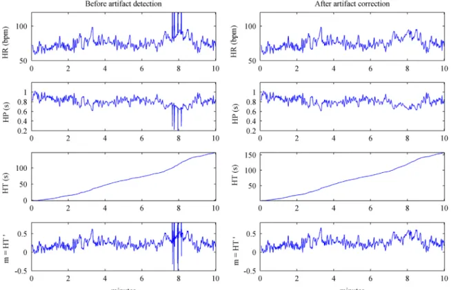
InFig. 1a period of 10 min is shown in which the different HRV source signals are displayed for a real subject. Notice the HT series

in this case is positive, meaning in this period the beat positions are positively deviated in reference to the mean RR interval. Last row in Fig. 1 shows the m(t) signal resulting from the differ-entiation of the HT series. As explained before, this is the actual signal that is used as input for the spectral analysis in the case of HT. Also, inFig. 1(left) an artifact is noticeable around the eighth minute affecting all the time series. In the samefigure (right) the resulting time series are shown once the artifacts have been corrected.

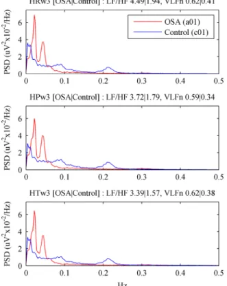
Fig. 2shows an example where the different spectra and the corresponding indices are presented for a patient in the OSA group (a01) and for a patient in the control group (c01) using the peri-odogram.Fig. 3shows the results for the same patients using the Welch approach. Only results using cubic splines are shown since the pattern in the case of 14th order splines is very similar. Two clear peaks are appreciable for the apneic patient in the VLF and low LF regions in contrast to the healthy case. The peak around 0.22 Hz observable in the control subject corresponds with the baseline respiratory frequency.

3.5. Classification

The objective here is to achieve the best possible separation between patients and controls on the basis of the different HRV features calculated as described in the previous sections.

In order tofind the best separating threshold, we use Receiver Operating Characteristic (ROC) curves. For that purpose we take the absolute maximum and minimum from each feature (LF/HF ratio, VLFn index) in the TR set and divide the space into 100 equidistant regions. The resulting frontier values are taken as the potential thresholds, and for each one the corresponding sensi-tivity and specificity values are computed. We thus obtain 100 different operating points in the ROC curve by plottingsensitivity in the ordinate and1-specificity in the abscissa. Using the ROC procedure we can compare each feature in terms of “general

separability”. At this respect, the area under the ROC curve (AUC) can be calculated. For that purpose we use a trapezoidal approx-imation using all the operating points (in our case 100) and computing the resulting area (AUC100). The best feature would be

the one with the highest AUC value. This is also known as theAUC criterion.

To perform subject classification then the optimal threshold in TR can be calculated for each feature by selecting the best single operating pointPAUC-bestin the corresponding ROC curve.PAUC-best can be calculated as the closest point(x,y)in Euclidean distance to the point (0,1). This point maximizes the quantity

(sensitivi-tyþspecificity)/2which is equivalent to the area under the triangle

connecting PAUC-bestwith the points (0,0) and (1,1). Notice

there-fore the same AUC criterion is being applied, but from the curve that results from one single operation point (instead of 100). The resulting threshold is then used to evaluate the separation per-formance both in TR and in TS.

Besides the ROC approach, a Naïve-Bayes (NB) classifier with kernel density estimation of the probably distribution function (pdf)is used for comparison purposes. Specifically, given a set ofnk i.i.d. data pointsfxk

ig

nk

i¼1drawn from a random variableXk, withpdf

(fk_x), its Parzen window estimate is:

d fkx;sk¼

1 nk

Xnk

i¼1

κ

k

xkiÞ ð11Þ

where

κ

k_xk

iÞis a kernel function with bandwidthsk. In our

case we use a Gaussian kernel, andskis approximated using the Silverman's rule:

sk¼1:06c

σ

5 ð12Þ

where

σ

nk

i¼1. The

subindexk refers in our case to the class indexk¼{0¼patients, 1¼controls}.

The resulting NB classifier is then trained using the TR set and tested using TS. Note, though, that in this case a numerical separating threshold cannot be obtained for which classification of a samplexk

i depends on the shape of its estimatedpdfwhich varies

over the domain ofXk.

It is worth to remark as well that the two above mentioned classification procedures offer robust solutions in the case of an unbalanced class problem such as in our case: n0¼20;n1¼10.

Prior probabilities in the case of NB classifier are nevertheless considered equiprobable to avoid bias of the classifier toward the most frequent class in the Apnea-ECG database.

3.6. Statistical analysis

In order to study statistical relevance of the different spectrum estimation methods, non-parametric Kruskal–Wallis test is used separately in the OSA and in the control group, to check whether the corresponding LF/HF or VLFn features from each method can be considered to come from different populations. Non-parametric test is used given that both Kolmogorov-Smirnov and Lilliefors tests, both at the 5% significance level, revealed general non-normality among the different populations. A multiple comparison test using the Tukey’s honestly significant difference criterion is applied to investi-gate pairwise effects. In addition, to test statistical significance between the OSA and the control groups, the Mann–Whitney U–test statistic is used for each derived feature.

4. Results

Table 2 shows mean threshold values between OSA patients and healthy controls within each method and for each feature, and shows the corresponding p-valuefor the Mann–Whitney U–test. Data is calculated over the whole dataset. Differences are con-sidered statistically significant (þ) when thep-valueis under the 0.05 significance level.

Fig. 2.Typical example of the resulting spectra and the corresponding LF/HF and VLFn indices for a patient in the OSA group (a01) and for a patient in the control group (c01) using the periodogram with cubic splines interpolation.

It can be seen fromTable 2that differences between patients and controls are mostly statistically significant regardless of the method used or the order of the splines. The exception is only among the LF/HF ratios derived from theHTw14spectrum. Then the difference does not reach statistical significance. The results support the hypothesis that there is actually a difference in the LF/ HF and VLFnfeatures between healthy controls and OSA patients regardless of the method chosen to compute the spectrum. Results in Table 2also indicate that these indices are in general higher among the OSA patients.

In general no statistical differences have been found using the Kruskal–Wallis test at the 0.05 significance level among the dif-ferent spectrum computations methods. Only statistical differ-ences have been found in the OSA group regarding the order of the splines (cubic vs 14th) when theHTwspectrum is used to calculate the LF/HF ratio (p-value¼0.01). The differences shown inTable 2

among the mean values of the different LF/HF and VLFn indices within each group (OSA or Controls) are irrelevant due to the associated (relatively high) variance.

From a classification perspective,Table 3shows the AUC values for each method resulting from the trapezoidal approximation of the ROC curve using 100 operating points as described inSection 3.5. From each ROC curve, the best separating threshold is also shown that corresponds to the single best operation point.

Tables 4and5show, respectively for the TR and the TS sets, the results regarding the classification of OSA and normal subjects according to the best thresholds shown inTable 3. For each table the corresponding values of sensitivity, speci_ficity, accuracy and AUC are shown. Notice the AUC value inTable 4may differ from the value AUC100 shown in Table 3 for which AUC values in Tables 4 and 5 correspond to the best individual (out of 100) operating points for each method.

Results fromTable 3show that the best ROC curve using the TR data is obtained for the LF/HF ratio when theHRw3spectrum is used with an overall AUC100value of 0.80. The best operating point

(reflecting the best balance between sensitivity and specificity) for this feature corresponds to a value threshold of 2.31. This results in classification sensitivity and specificity in TR of 0.75 and 0.80 respectively, and in TS of 0.85 and 0.70. The specific AUC values corresponding to this operating point, as it can be seen in

Tables 4and5, are 0.78 for TR and 0.77 for TS. However, if we take as reference the best AUC values in these tables, it can be seen that the maximum classification performance for the LF/HF ratio, is achieved by using theHRP3spectrum, with an associated classifi -cation threshold of 3.17. Table 5shows that using the previous combination of method and threshold, the AUC value in TS set

increased to 0.88 (in TR the value is maintained in 0.78). Globally, however, the area under the ROC curve in the case of HRP3 is inferior (AUC100¼0.70) with respect toHRw3(AUC100¼0.80).

The classification performance associated to the LF/HF feature usingHRP3is also the best achieved overall (i.e. taking into account also performances achieved by the VLFnfeature). For the VLFnfeature, the best threshold derived from the ROC area inTable 3corresponds to the HPw3 spectrum, with an AUC100 of 0.78 and an associated

threshold for the OSA group of 0.49. Using this threshold a classifi -cation performance of 0.80 is obtained in terms of AUC for TR, and of 0.70 for TS (seeTables 4 and5respectively). The best classification performance however is obtained for TR using theHRwspectrum (AUC of 0.85 regardless the order of the splines), and for TS using theHTP spectrum (AUC of 0.77, again both for cubic and for 14th-order splines).

Finally Table 6shows the performance results when the NB classifier is used. Only the results for the TS test are shown because

Table 2

Differences in the LF/HF and VLFnindices between OSA patients and Controls in the whole dataset. Data is shown as mean and standard deviation (in parentheses).

SP3¼results with cubic splines interpolation; SP14¼results with 14th order splines interpolation.

Feature Method OSA Controls p-Value (OSA vs Controls)

Sp3 Sp14 Sp3 Sp14 Sp3 Sp14

LF/HF HRP 5.25 (4.22) 4.64 (4.11) 1.89 (0.84) 1.70 (0.85) 0.0002þ 0.0005þ

HRW 4.78 (3.53) 4.10 (3.52) 1.92 (0.86) 1.75 (0.82) o0.0001þ 0.0014þ

HPP 4.21 (3.60) 3.87 (3.52) 1.73 (0.82) 1.61 (0.79) 0.0001þ 0.0003þ

HPW 3.74 (2.76) 3.35 (2.76) 1.79 (0.88) 1.67 (0.85) 0.0001þ 0.0010þ

HTP 4.14 (3.25) 3.86 (3.21) 1.65 (0.78) 1.47 (0.79) 0.0003þ 0.0006þ

HTW 3.39 (2.35) 2.41 (1.89) 1.62 (0.76) 1.48 (0.72) 0.0002þ 0.0889

VLFn HRP 0.65 (0.14) 0.65 (0.14) 0.47 (0.21) 0.46 (0.22) 0.0014þ 0.0013þ

HRW 0.72 (0.11) 0.70 (0.13) 0.53 (0.21) 0.51 (0.21) 0.0005þ 0.0007þ

HPP 0.62 (0.15) 0.61 (0.15) 0.41 (0.20) 0.41 (0.19) 0.0003þ 0.0003þ

HPW 0.67 (0.12) 0.66 (0.13) 0.46 (0.20) 0.45 (0.19) 0.0001þ 0.0001þ

HTP 0.64 (0.13) 0.61 (0.18) 0.47 (0.18) 0.44 (0.21) 0.0005þ 0.0013þ

HTW 0.70 (0.11) 0.62 (0.20) 0.51 (0.21) 0.49 (0.22) 0.0012þ 0.0235þ

Table 3

in general, when the NB approach is used, no significant improvement is achieved over the results of the ROC analysis. The structure ofTable 6is identical to that ofTables 4and5.

Indeed, when using cubic splines, the best classification per-formances with the NB classifier are achieved with the LF/HF ratio using both theHRP(irrelevant order of the splines) and theHPP3 spectra, but with an inferior AUC value as with respect to the best value achieved using the ROC approach (0.82 for NB inTable 6vs 0.88 for ROC in Table 5). For the VLFn feature, using the NB approach the best performance is achieved using either theHRor theHTspectra. The order of the splines does not influence again the results. The best AUC value in this case (0.77) equals the one achieved by the ROC analysis (see HTPfor VLFninTables 5and6).

5. Discussion

We have explored the utility of HRV spectral-based features, namely the LF/HF ratio and the VLFnindex, obtained from different

spectrum estimation methods, for the screening of patients with SAHS. Moreover, our main purpose was to assess the suitability of the IPFM-derived HT signal as the source of spectral analysis in comparison to the classical HR or HP signals. The interest origi-nates given the theoretical minimal distortion introduced in the spectrum of the former to reflect the regulatory modulation mechanisms involved in the HRV[25,35].

Our statistical results have revealed that by means of the pro-cedures followed in this work, and at least regarding the Apnea-ECG database, the choice between any of these three source sig-nals (HR, HP or HT) would not signi_ficantly affect the derived markers of LF/HF and VLFn.

Also these markers would not be affected by the order of the splines used to interpolate the unevenly-spaced beat series (cubic or 14th-order). The use of high order splines would contribute to minimize the low-passfilter effects introduced by the HR and the HP based estimations, thus favoring a more reliable spectrum estimate in the case of HT, especially at the highest frequencies

[25,35]. This improvement, however, has proven in practice not to be relevant for the computation of the above mentioned features. The use of the regular periodogram or of the Welch spectrum has not shown a significant effect either.

In our experiments appropriate detection and correction of arti-facts, including ectopic beats, has been identi_fied to be a fundamental step to obtain reliable spectral estimates. Our experiments have shown statistical differences within each source signal, before and after the correction of the artifacts. These results have not been shown here to simplify the analysis; however, the result is interpreted as a positive effect of the artifact detection procedure, getting rid of spurious values that were actually corrupting the estimated spectra. Actually it is only after artifacts have been processed that differences in the derived features become statistically negligible. Imposing a limit to the inter-polation gap was absolutely necessary at this respect. Strangely enough, none of the previous approaches that we know of in the lit-erature that interpolate the unevenly spaced samples of the HRV source signal explicitly mention this issue [9,12,13,15–19,21,22,24].

Table 4

Classification performance in TR using the ROC approach for the LF/HF and the VLFn features. The thresholds corresponding to the best operation points referenced in Table 3are used. SP3¼results with cubic splines interpolation; SP14¼results with 14th order splines interpolation. Best performance points according to the AUC criterion are highlighted with a gray background for each combination of feature and interpolation order. Best absolute performance is indicated in bold.

Table 5

Classification performance in TS using the ROC approach for the LF/HF and the VLFn

features. The thresholds corresponding to the best operation points referenced in Table 3are used. SP3¼results with cubic splines interpolation; SP14¼results with 14th order splines interpolation. Best performance points according to the AUC criterion are highlighted with a gray background for each combination of feature and interpolation order. Best absolute performance is indicated in bold.

Table 6

Classification performance in TS using the NB approach for the LF/HF and the VLFn

Nevertheless, in practice it is common that artifacts affecting ECG recordings could easily extend for several seconds, if not minutes, causing big interpolation gaps. Such intervals gaps should be handled to avoid the corresponding interpolated output to contaminate the resulting spectral estimate.

The statistical analysis has shown, on the other hand, that there is a significant difference in the values obtained for the LF/HF ratio and VLFnindex between OSA patients and healthy controls. This supports,

in principle, the idea of using spectral features based on the standard HRV bands as relevant markers for the OSA screening. The statistical analysis did show as well that in the tested database these indices are higher in the OSA group. This result has consistently been reported in previous works using the Apnea-ECG database[20–24], and also in general for most of the studies using different databases [6,8,9,12– 15,17–19,21,23,24]. One commonly reported interpretation is that the presence of apneic events would influence the autonomic regulation because of the stress produced by the lack of oxygen in arterial blood, generating an arousal response, shifting to a dominance of the sym-pathetic control. This would be reflected in a relative increase of the normalized LF component, while the normalized HF component would decrease as the respiration becomes irregular and the para-sympathetic regulation losses control. Patients with SAHS would thus tend to have an increased LF/HF ratio. As with regard to the observed increase on the VLF component, the interpretation is more proble-matic since technically VLF is not regulated by the sympathetic ner-vous system[7]. Perhaps a better explanation should lay its founda-tion, not in terms of intrinsic autonomic activity, but on the periodicity of the changes induced in HR because of the periodic appearance of apneic events in the VLF associated frequency. Discussion is still on the table, so caution needs to be applied in interpreting the above results

[4]. Moreover, literature is not always consistent, and some works can be found where the previous trends do not hold across all the severity groups or sleep stages[10,11], or that even have reported lower values of these indices for the OSA group.[16].

We have further tested the separability hypothesis by attempt-ing subject classi_fication on the basis of the derived HRV features. The objective was to test how the differences found in the spectral features translate to the patient classification task. In this respect, our results only moderately support such hypothesis with AUC values in the testing set ranging 0.53–0.88, depending on the dis-criminating feature and on the spectral estimation method. Within this range the LF/HF ratio can achieve better performance but it also presents higher variability (0.53–0.88) than the VLFnfeature (0.60–

0.77). In addition, the use of cubic splines shows better (0.60–0.88) than the use of 14th-order splines (0.53–0.85), and the Welch spectrum provides worst results (0.53–0.78) than the periodogram (0.72–0.88). Among the three tested source signals, the HR seems in general to obtain the best results (0.63–0.88), with HP varying 0.60–

0.80 and HT 0.53–0.80. The best absolute performance in terms of AUC was obtained by the LF/HF feature derived from the HRw3 spectrum. Recall, nonetheless, that the statistical analysis has not supported the existence of relevant differences among the derived features. Actually, from the analysis of the results inTables 3–6, we resolve that it is difficult to see a clear trend that shows a method to be superior to the rest in terms of classification performance.

When analyzing previous works in the literature using standard HRV spectral bands definition, the work of Hiltonet al.can be men-tioned in which the authors obtain AUC values for the LF/HF ratio of 0.62 in REM and 0.71 in NREM using a proprietary database and the HP signal[19]. Using the Apnea-ECG database, Hoessen et al. used the LF/HF ratio derived from the HP signal and achieved AUC of 0.90 over the whole dataset. They used a soft-decision algorithm for spectral subband decomposition[21]. With the same data partition, Ladoet al. obtained 0.90 sensitivity for the OSA class, but reached only 0.40 accuracy for the classification of the normal cases. In this work the authors made use of the HR signal. In a previous preliminary study

using the Apnea-ECG database we have obtained an AUC of 0.55 in the testing set when using the LF/HF ratio derived from the HP signal

[24]. In the same work, however, we were able to improve the per-formance up to an AUC of 0.78 when a custom LF/HF ratio was used derived from non-HRV standard spectral bands. Indeed, the literature seems to support the possibility of achieving better performance when spectral features are calculated ad-hoc, i.e. without sticking to the standard HRV band definitions. This is for example the case in the work of Drinnan et al., which using also the Apnea-ECG database achieved a classi_fication AUC of 0.93 with a tachogram-based LF/HF feature derived from a customized definition of the LF and HF bands

[20]. The work of Oteroet al.can be mentioned as well, which using the same database and the HP signal, achieved an AUC of 0.98 in the testing set with a feature based on the ratio between the 0.026–

0.06 Hz and the 0.06–0.25 Hz bands [22]. A side effect of ad-hoc features is though the absence of a standard clinical framework for their interpretation.

As far as we know, no previous attempts have been made to classify OSA patients and controls using the VLF band alone. Only in the previously mentioned work of Hoessenet al.the authors tested the use of a feature based on the LF/VLF ratio, obtaining similar results in comparison to the LF/HF ratio[21]. Also previously mentioned, in the work of Hiltonet al.,but using a different database than the Apnea-ECG, the AUC values are increased with respect to the standard LF/HF ratio up to 0.85 in REM and 0.77 in NREM when using the power in the 0.019_–0.036 Hz band[19]. Note this custom feature is included in the upper half of the standard VLF definition.

Limitations of the present study include, for example, the fact that when spectral analysis is performed during long periods affecting the LF and the HF bands, the stationarity condition cannot be guaranteed. Also for the purposes of HRV spectral analysis, averaging of spectral results from shorter segments (e.g. 5 min), is in general discouraged. In this respect averages of the modulations attributable to the LF and HF components may obscure detailed information about autonomic regulation available in non-averaged short recordings.[5].

For the interpretation of our results, the reader should also take into account that the actual signal modulating the heart rate activity is, of course, unknown. Theoretical optimality of HT for spectral analysis only holds under the IPFM assumption, but still there is no proof that the IPFM model can explain all the com-plexity of the beat generation process.

Finally, it must be remarked that the results here obtained refer to the Apnea-ECG database and cannot be made extensible to other databases. Some previous works in this respect, have already warned about the instability of some HRV spectral features, including the LF/ HF ratio, when changing the source database.[23,24].

Future work will address indeed a more extensive study increasing the number of databases to analyze the robustness of the indices obtained in this work (including those derived from the HT signal) to the effect of database variability.

6. Conclusion

The fact that the HT signal is supported and derived from a physiological-inspired mathematical model such as the IPFM makes the use of this signal interesting in practice. In this work we have shown how the HT signal can be used in an applied domain, in this case, the screening of SAHS. Comparability analysis of spectral HRV indices derived from HT and the classical sources of HR and HP have shown similar outcomes in the Apnea-ECG database. Slight variations over these indices have not reached statistical relevance. Patient classification results, on the other hand, only moderately support the viability of using the spectral features of VLFnand LF/HF based on the

task, better performance can be achieved when using features derived from custom spectral bands. Future work should assess the con-sistency of our findings and their replicability when different and more heterogeneous databases are used.

Conflicts of interest statement

None declared.

Acknowledgment

Research funded in part by Spanish Xunta de Galicia under research projects CN2011/007 and CN2012/211, partially supported by European Union ERDF funds, and by Spanish MINECO under research project TIN2013-40686-P. The authors would like to grate-fully thank Dr. Javier Mateo for his useful comments during the development of this work.

References

[1]T. Young, et al., The occurrence of sleep-disordered breathing in middle-aged adults, N. Engl. J. Med. 328 (1993) 1230–1235.

[2]C. Guilleminault, S. Connolly, R. Winkle, K. Melvin, A. Tilkian, Cyclical variation of the heart rate in sleep apnoea syndrome. Mechanisms and usefulness of 24h electrocardiography as a screening technique, Lancet 1 (1984) 126–131. [3]T. Penzel, et al., Systematic comparison of different algorithms for apnoea

detection based on electrocardiogram recordings, Med. Biol. Eng. Comput. 40 (2002) 402–407.

[4]P.K. Stein, Y. Pu, Heart rate variability, sleep and sleep disorders, Sleep Med. Rev. 16 (2012) 47–66.

[5]M. Malik, et al., Heart rate variability: standards of measurement, physiological interpretation and clinical use. Task Force of the European Society of Cardi-ology and the North American Society of Pacing and ElectrophysiCardi-ology, Cir-culation 93 (5) (1996) 1043–1065.

[6]T. Shiomi, et al., Augmented very low frequency component of heart rate variability during obstructive sleep apnea, Sleep 19 (5) (1996) 370–377. [7]J.A. Taylor, D.L. Carr, C.W. Myers, D.L. Eckberg, Mechanisms underlying very-low

frequency RR-interval oscillations in humans, Circulation 98 (1998) 547–555. [8]K. Narkiewicz, et al., Altered cardiovascular variability in obstructive sleep

apnea, Circulation 98 (1998) 1071–1077.

[9]M.C.K. Khoo, T.S. Kim, R.B. Berry, Spectral indices of cardiac autonomic func-tion in obstructive sleep apnea, Sleep 22 (4) (1999) 443–451.

[10]L.J. Gula, et al., Heart rate variability in obstructive sleep apnea: a prospective study and frequency domain analysis, Ann. Noninvasive Electrocardiol. 8 (2) (2003) 144–149.

[11]T. Penzel, J.W. Kantelhardt, L. Grote, J.H. Peter, A. Bunde, Comparison of detrendedfluctuation analysis and spectral analysis for heart rate variability in sleep and sleep apnea, IEEE Trans. Biomed. Eng. 50 (10) (2003) 1143–1151. [12]F. Roche, S. Celle, V. Pichot, J.C. Barthélémy, E. Sforza, Analysis of the interbeat

interval increment to detect obstructive sleep apnoea/hypopnoea, Eur. Respir. J. 29 (2007) 1206–1211.

[13]E. Sforza, F. Chouchou, V. Pichot, J.C. Barthélémy, F. Roche, Heart rate incre-ment in the diagnosis of obstructive sleep apnoea in an older population, Sleep Med. 13 (2012) 21–28.

[14]E. Vanninen, A. Tuunainen, M. Kansanen, M. Uusitupa, E. Länsimies, Cardiac sympathovagal balance during sleep apnoea episodes, Clin. Physiol. 16 (3) (1996) 209–216.

[15]K. Dingli, et al., Spectral oscillations of RR intervals in sleep apnoea/hypopnoea syndrome patients, Eur. Respir. J. 22 (2003) 943–950.

[16]A.H. Khandoker, C.K. Karmakar, M. Palaniswami, Comparison of pulse rate variability with heart rate variability during obstructive sleep apnea, Med. Eng. Phys. 33 (2011) 204–209.

[17]K. Zhu, et al., Overnight heart rate variability in patients with obstructive sleep apnoea: a time and frequency domain study, Clin. Exp. Pharmacol. Physiol. 39 (2012) 901–908.

[18]M.J. Lado, A.J. Méndez, L. Rodríguez-Liñares, A. Otero, X.A. Vila, Nocturnal evolution of heart rate variability indices in sleep apnea, Comput. Biol. Med. 42 (2012) 1179–1185.

[19]M.F. Hilton, R.A. Bates, K.R. Godfrey, M.J. Chappell, R.M. Cayton, Evaluation of fre-quency and time-frefre-quency spectral analysis of heart rate variability as a diagnostic marker of the sleep apnoea syndrome, Med. Biol. Eng. Comput. 37 (1999) 760–769. [20] M.J. Drinnan, J. Allen, P. Langley, A. Murray, Detection of sleep apnoea from

fre-quency analysis of heart rate variability, Comput. Cardiol. 27 (2000) 259–262. [21]A. Hossen, B.A. Ghunaimi, M.O. Hassan, Subband decomposition soft-decision

algorithm for heart rate variability analysis in patients with obstructive sleep apnea and normal controls, Signal Process. 85 (2005) 95–106.

[22] A. Otero, S.F. Dapena, P. Felix, J. Presedo, M. Tarasco, A low cost screening test for obstructive sleep apnea that can be performed at the patient’s home, in: Proceedings of IEEE International Symposium on Intelligent Signal Processing, Budapest, 2009, pp. 199–204.

[23] M.J. Lado, et al., Detecting sleep apnea by heart rate variability analysis: assessing the validity of databases and algorithms, J. Med. Syst. 35 (2011) 473–481. [24] V. Peiteado-Brea, D. Alvarez-Estevez, V. Moret-Bonillo, A study of heart rate

variability as sleep apnoea predictor over two different databases, in: Pro-ceedings of IEEE-EMBS International Conference on Biomedical and Health Informatics, Valencia, 2014, pp. 359–362.

[25] J. Mateo, P. Laguna, Improved heart rate variability signal analysis from the beat occurrence times according to the IPFM model, IEEE Trans. Biomed. Eng. 47 (8) (2000) 985–996.

[26] E.J. Bayly, Spectral analysis of pulse frequency modulation in the nervous systems, IEEE Trans. Biomed. Eng. 15 (1968) 257–265.

[27] R.D. Berger, S. Akeselrod, D. Gordon, R.J. Cohen, An efficient algorithm for spectral analysis of heart rate variability, IEEE Trans. Biomed. Eng. 33 (1986) 900–904.

[28] P.E. McSharry, G.D. Clifford, Models for ECG and RR intervals processes, in: G. D. Clifford, F. Azuaje, P.E. McSharry (Eds.), Advanced Methods and Tools for ECG Data Analysis, Artech House, Boston, 2006, pp. 101–133.

[29] T. Penzel, et al., The Apnea-ECG database, Comput. Cardiol. 27 (2000) 255–258. [30] Detecting and Quantifying Apnea Based on the ECG: A Challenge From

Phy-sioNet and Computers in Cardiology 2000.〈https://physionet.org/challenge/ 2000/〉January, 2016.

[31]S. Babaeizadeh, D.P. White, S.D. Pittman, S.H. Zhou, Automatic detection and quantification of sleep apnea using heart rate variability, J. Electrocardiol. 43 (2010) 535–541.

[32] P. de Chazal, et al., Automated processing of the single-lead electrocardiogram for the detection of obstructive sleep apnoea, IEEE Trans. Biomed. Eng. 50 (6) (2003) 686–696.

[33] M.O. Mendez, A.M. Bianchi, M. Matteucci, S. Cerutti, T. Penzel, Sleep apnea screening by autoregressive models from a single ECG lead, IEEE Trans. Biomed. Eng. 56 (12) (2009) 2838–2850.

[34] S. Akselrod, et al., Power spectrum analysis of heart rate fluctuation: a quantitative probe of beat-to-beat cardiovascular control, Science 213 (4504) (1981) 220–222.

[35] J. Mateo, P. Laguna, Analysis of heart rate variability in the presence of ectopic beats using the heart timing signal, IEEE Trans. Biomed. Eng. 50 (3) (2003) 334–343. [36] V.X. Alfonso, W.J. Tompkins, T.Q. Nguyen, S. Luo, ECG beat detection using

filter banks, IEEE Trans. Biomed. Eng. 46 (2) (1999) 192–202.

Diego Alvarez-Estevezwas born in Ourense, Spain, in 1982. He graduated in Computer Science Engineering at University of A Coruña, Spain, in 2007. In 2012 he obtained his PhD (cum laude) on the application of artificial intelligence techniques to the diagnosis of the Sleep Apnea-Hypopnea Syndrome. In 2013 he joined the Sleep Center of the Medisch Centrum Haaglanden in The Hague, The Netherlands. His current research interests include computer-based sleep research, machine learning and biomedical signal processing.