Structural optimization in atomic systems with few degrees of freedom

Texto completo

(1)SISTEMA UNIVERSITARIO ESTATAL SUE CARIBE UNIVERSIDAD DE CARTAGENA MAESTRÍA EN CIENCIAS FÍSICAS. STRUCTURAL OPTIMIZATION IN ATOMIC SYSTEMS WITH FEW DEGREES OF FREEDOM Beatriz Helena Cogollo Olivo. Thesis submitted for Advisor the degree of Javier Antonio Master in Physical Montoya Martínez, Sciences Ph. D.. Cartagena de Indias, D. T. y C. 2014.

(2) STRUCTURAL OPTIMIZATION IN ATOMIC SYSTEMS WITH FEW DEGREES OF FREEDOM. BEATRIZ HELENA COGOLLO OLIVO. UNIVERSITY OF CARTAGENA MASTER IN PHYSICAL SCIENCES SUE – CARIBE CARTAGENA DE INDIAS, D. T. Y C. COLOMBIA 2014.

(3) STRUCTURAL OPTIMIZATION IN ATOMIC SYSTEMS WITH FEW DEGREES OF FREEDOM. Thesis submitted for the degree of Master in Physical Sciences. BEATRIZ HELENA COGOLLO OLIVO. ADVISOR Javier Antonio Montoya Martínez, Ph.D.. UNIVERSITY OF CARTAGENA MASTER IN PHYSICAL SCIENCES SUE-CARIBE CARTAGENA DE INDIAS, D. T. Y C. COLOMBIA 2014.

(4) Cartagena de Indias, 9 de Diciembre de 2014. Señores Miembros Comité Curricular de la Maestría en Ciencias Físicas SUE Caribe. Estimados Señores Miembros del Comité, Tengo el agrado de dirigirme a ustedes a fin de solicitarles sea evaluada el Trabajo de Grado de Maestría, titulada “STRUCTURAL OPTIMIZATION IN ATOMIC SYSTEMS WITH FEW DEGREES OF FREEDOM”, de la cual adjunto dos (2) copias impresas y una (1) en formato electrónico CD. Saluda a ustedes, muy atentamente.. BEATRIZ HELENA COGOLLO OLIVO Estudiante Programa de Maestría en Ciencias Físicas SUE- Caribe. Visto Bueno: JAVIER ANTONIO MONTOYA MARTÍNEZ Docente – Facultad de Ciencias Exactas y Naturales Universidad de Cartagena. Visto Bueno: LUIS EDUARDO CORTÉS RODRÍGUEZ Coordinador Institucional Maestría en Ciencias Físicas Universidad de Cartagena.

(5) AKNOWLEDGEMENTS. This is one more step of a journey called life. Today I'm writing these lines because several people believed and supported me and this work is for them. First, I want to thank deeply my advisor, Prof. Javier Montoya. He's the reason for me to be here, growing not only as a scientist but also as a person. I'm completely grateful to him for encouraging me to pursue a path of excellence and I'm very proud to count on him not only as a tutor, but also as a friend and role model. I was, and still am, very lucky to have such a supportive family: Morales, mom, dad and "Pre", thanks a lot for all your efforts! Thank you for being there and for supporting me in this new path, even when some of you don't have a very clear idea of why the world needs physicists. Thanks to my dearest friend Melisa, we were able to contemplate and enjoy the beauty of nature, and she made me realize every time we talked about what I was doing, that I finally found my passion. Through my words she saw a glimpse of the marvelous of our universe and I fell in love with science again and again. And finally to all those that I haven't mention, professors and research group colleagues, I'm sure that your ideas, comments or discussions at some point of this M. Sc. program helped me to reach to this point, thank you all.. Beatriz December, 2014.

(6) “(…) take the point of a pencil and magnify it. One reaches the point where a stunning realization strikes home: The pencil is not solid; it is composed of atoms which whirl and revolve like a trillion demon planets. What seems solid to us is actually only a loose net held together by gravitation.”. Stephen King. The Dark Tower Series – Book 1: The Gunslinger.

(7) CONTENTS p. List of Tables. i. List of Figures. ii. List of Annexes. v. Abstract. vi. CHAPTER 1: THEORETICAL FOUNDATION CRYSTAL STRUCTURE PREDICTION PROBLEM. 1. METHODS OF CRYSTAL STRUCTURE PREDICTION. 4. Random Sampling. 6. Simulated Annealing. 7. Molecular Dynamics. 8. Metadynamics. 10. Evolutionary Algorithms. 11. THE ELECTRONIC PROBLEM. 12. Born – Oppenheimer Approximation. 13. Hartree and Hartree – Fock Approximations. 15. Thomas – Fermi Theory. 19. Hohenberg – Kohn Theorems. 21. Kohn – Sham Method. 24. Exchange and Correlation in DFT. 27. Local Density Approximation – LDA. 28. Generalized Gradient Approximation – GGA. 29. Pseudopotentials and Basis Sets. 31. Pseudopotentials. 32. Basis Sets. 34. REFERENCES. 35.

(8) CHAPTER 2: STUDY CASE: SOLID OXYGEN AT HIGH PRESSURE STATE OF THE ART. 41. Phases of solid oxygen in equilibrium with vapor. 42. High – pressure phases of solid oxygen. 43. METHODOLOGY. 47. TECHNICAL DETAILS. 48. RESULTS. 51. Molecular Solid Oxygen. 51. Monoatomic Oxygen (Special Case). 64. DISCUSSION AND CONCLUSIONS. 66. REFERENCES. 69. CHAPTER 3: STUDY CASE: COPPER CLUSTERS IN VACUUM OVERVIEW ON CLUSTERS. 74. TRANSITION METAL CLUSTERS. 75. Shell effects and magic numbers. 75. Clusters Band Gap. 76. STATE OF THE ART Isomers. 77 78. METHDOLOGY. 81. TECHNICAL DETAILS. 82. RESULTS. 84. DISCUSSION AND CONCLUSIONS. 89. Geometry of ground state and isomers structures. 89. Binding Energies. 90. HOMO – LUMO Gap. 92. REFERENCES. 93. Closing Remarks. 97. APPENDIX A. DIRAC’S NOTATION AND SECOND QUANTIZATION. 99.

(9) LIST OF TABLES. p. Table 1.1. Microscopic properties of crystal materials.. 2. Table 1.2. Several algorithms used in Molecular Dynamics.. 9. Table 1.3. Expressions used to calculate the exchange-correlation energy in LDA.. 29. Table 1.4. Summary of several GGA functionals.. 31. Table 2.1. Parameters used in the Quantum ESPRESSO input files for oxygen structural search.. 50. Table 2.2. O2 structures that converged into a local minima.. 52. Table 2.3. O4 structures that converged into a local minima.. 53. Table 2.4. Cell parameters for equivalent structures for O2 at pressures from 0.35 to 3.5 TPa.. 54. Table 2.4. Cell parameters for equivalent structures for O2 at pressures from 0.35 to 3.5 TPa. (Cont.). 55. Table 2.5. Cell parameters for equivalent structures for O4 at pressures from 0.5 to 3.5 TPa.. 55. Table 2.5. Cell parameters for equivalent structures for O4 at pressures from 0.5 to 3.5 TPa. (Cont.). 56. Table 2.5. Enthalpy values for several monoatomic oxygen structures from 1TPa to 8TPa.. 61. Table 3.1 Classification of clusters according to size. N is the number of atoms, D is the diameter (for a cluster of sodium atoms) and FS is the fraction of surface atoms.. 74. Table 3.2. Symmetry group of Cun clusters (n = 3 – 7). 79. Table 3.2. Symmetry group of Cun clusters (n = 3 – 7). (Cont.). 80. Table 3.3. Binding energy in [eV/atom] of Cun clusters (n = 3 – 7).. 81. Table 3.4. Parameters used in the Quantum ESPRESSO input files for copper clusters structural search.. 84. Table 3.5. Binding energy (BE) and difference in binding energy (E) of ground state an isomers of Cun (n = 3 – 7).. 89. i.

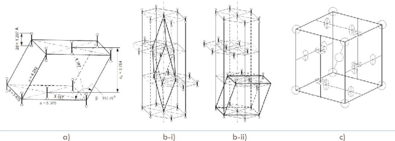
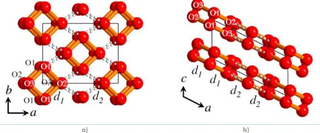
(10) LIST OF FIGURES. p. Figure 1.1. Proposed methods for solving the crystal structure prediction problem.. 4. Figure 1.2. Energy landscape. It contains kinetics traps and energy barrels.. 6. Figure 1.3. Simplified version of a Random Sampling algorithm.. 7. Figure 1.4. Schematic representation of simulated annealing.. 8. Figure 1.5. Particle trajectory in Molecular Dynamics simulation.. 9. Figure 1.6. Schematic representation of the progressive filling of the underlying potential (thick line) by means of the Gaussians deposited along the trajectory. The sum of the underlying potential and of the metadynamics bias is shown at different times (thin lines).. 11. Figure 1.7. Self-Consistent Field (SCF) algorithm.. 18. Figure 1.8. The Fermi sphere with an infinitesimal volume of dp3 in the real space, or (2π/L)3 in the K-space.. 19. Figure 1.9. Schematic representation of Hohenberg-Kohn Theorem.. 21. Figure 1.10. Schematic illustration of all-electron (solid lines) and pseudoelectron (dashed lines) potentials and their corresponding wave functions. The radius at which all-electron and pseudoelectron values match is designated rc.. 33. Figure 1.11. Flow chart describing the construction of an ionic pseudopotential for an atom. 34 Figure 2.1. Phase diagram of solid oxygen.. 42. Figure 2.2. Structure of solid oxygen at a) -phase; -phase in b-i) rhombohedral axes and b-ii) monoclinic axes; c) -phase, where circles represent the orientational disorder of the molecules.. 43. Figure 2.3. Structure of -oxygen.. 43. Figure 2.4. A possible arrangement of molecules at the bc face of the A2/m unit cell of O2.. 44. Figure 2.5. Proposed structural model of -O2 at 11.4 GPa viewed along a) the c and b) the b axes.. 45. Figure 2.6. Proposed new phase diagram of oxygen.. 46. ii.

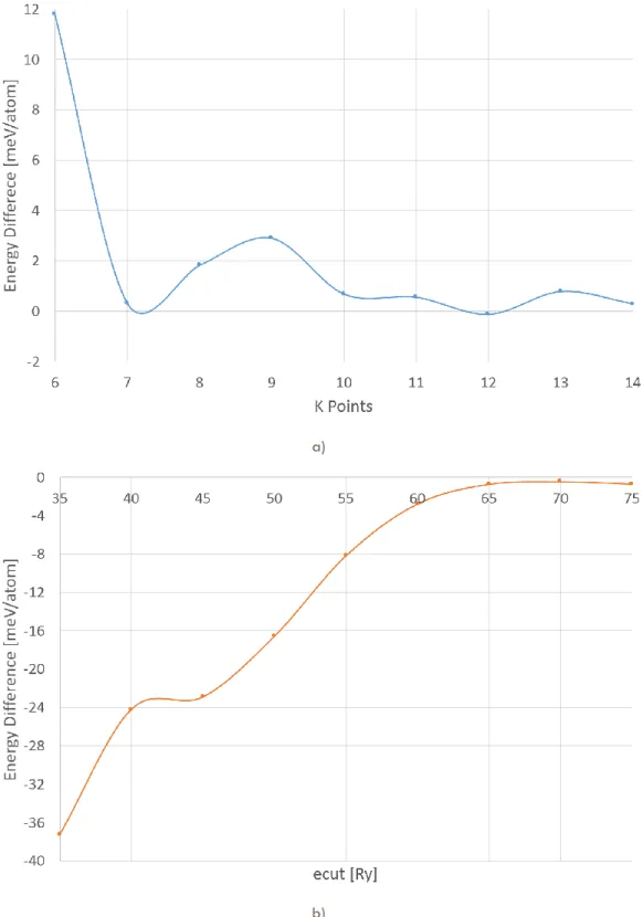
(11) Figure 2.7. Energy convergence for an O2 structure at 3500GPa. Varying a) k-points grid and b) plane wave kinetic cutoff.. 49. Figure 2.8. Energy convergence for an O4 structure at 3500GPa. Varying a) k-points grid and b) plane wave kinetic cutoff.. 50. Figure 2.9. Enthalpy variation for O2 at pressures from 0.35 to 3.5 TPa. For each pressure, the circle size is proportional to the number of initial structures that converged to the marked enthalpy.. 52. Figure 2.10. Enthalpy variation for O4 at pressures from 0.5 to 3.5 TPa. For each pressure, the circle size is proportional to the number of initial structures that converged to the marked enthalpy.. 53. Figure 2.11. Equivalent structures for O2 at pressures from 0.35 to 3.5 TPa.. 56. Figure 2.11. Equivalent structures for O2 at pressures from 0.35 to 3.5 TPa. (Cont.). 57. Figure 2.11. Equivalent structures for O2 at pressures from 0.35 to 3.5 TPa. (Cont.). 58. Figure 2.11. Equivalent structures for O2 at pressures from 0.35 to 3.5 TPa. (Cont.). 59. Figure 2.12. Equivalent structures for O4 at pressures from 0.5 to 3.5 TPa.. 59. Figure 2.12. Equivalent structures for O4 at pressures from 0.5 to 3.5 TPa. (Cont.). 60. Figure 2.12. Equivalent structures for O4 at pressures from 0.5 to 3.5 TPa. (Cont.). 61. Figure 2.13. Volume evolution while pressure increases. a) O2 system. b) O4 system.. 62. Figure 2.14. Evolution of first (blue), second (orange) and third (green) neighbors distances while pressure increases. a) O2 system structures: P-1 (triangles), C2/m (squares) and Cmcm (circles). b) O4 system structures: Cmma (rhombus) and Cmcm (circles).. 63. Figure 2.15. Enthalpy difference for several monoatomic oxygen structures from 1TPa to 8 TPa. Fmmm structure is the reference.. 65. Figure 2.16. Zigzag chains for a) O2 and b) O4.. 66. Figure 2.17. Enthalpy per atom of the most stables structures of O2 and O4 systems from 0.35 to 1.50 TPa. The symmetry groups are labeled as: Cmma (squares), P-1 (rhombus), C2-m (triangles), and Cmcm (circles).. 67. Figure 2.18. Layered structure for a) O2 and b) O4.. 68. Figure 3.1. Schematic comparison between band gaps of different sizes of copper clusters (blue tones) and several semiconductors (orange bars).. 76. Figure 3.2. Total energy convergence for a Cu3 cluster. Varying a) k-points grid, b) plane wave kinetic cutoff and c) cubic unit-cell edge length.. iii. 83.

(12) Figure 3.3. Energy evolution of: a) Cu3 (red line), b) Cu4 (blue line). For each size, the first region is the ground state structure, and the subsequent represent a cluster isomer.. 85. Figure 3.3. Energy evolution of: c) Cu5 (orange line), d) Cu6 (green line. For each size, the first region is the ground state structure, and the subsequent represent a cluster isomer. (Cont.). 86. Figure 3.3. Energy evolution of: e) Cu7 (yellow line). For each size, the first region is the ground state structure, and the subsequent represent a cluster isomer. (Cont.). 87. Figure 3.4. Structures found for Cu3, Cu4, Cu5, Cu6 and Cu7.. 88. Figure 3.5. Comparison of binding energy per atom as a function of cluster size, among: our results using DF-GGA (red), DF-LDA [23] (blue), TB [25] (green), Real Space Pseudopotential [27] (yellow), MD [28] (orange) and two CID experiments [21] [22] (dashed lines grey and violet).. 91. Figure 3.6. Evolution of the highest occupied – lowest occupied (HOMO – LUMO) gap energy as the cluster size increases.. 92. iv.

(13) LIST OF APPENDIXES. p. Appendix A. Dirac’s Notation and Second Quatization. v. 99.

(14) Chapter 1 Theoretical Foundation. Chapter 1 T H E O R E T I C A L F O U N DAT I O N. CRYSTAL STRUCTURE PREDICTION PROBLEM The crystal structure prediction (CSP) is a problem that has attracted the scientific community’s attention since the establishment of the first set of Pauling's Rules in 1929. This problem can be resumed as follows: given only the chemical composition of any material there exist an infinite amount of atomic arrangements that can be obtained, each one of them with a certain total energy inside the configurational energy landscape. Therefore, the crystal structure prediction problem consists in finding, for some external conditions, e.g. a given applied pressure and/or temperature, the most stable structure i.e. the one with the lowest free energy, starting only from the knowledge of the chemical composition of the system [1]. Almost sixty years later, in 1988, there were very few advances for the solution of this problem; the famous editorial by John Maddox [2] resumes the situation at that time:. “One of the continuing scandals in the physical sciences is that it remains in general impossible to predict the structure of even the simplest crystalline solids from a knowledge of their chemical composition”. Then, it is natural to ask ourselves why it is so important to determine the crystal structure of a crystalline system. The answer is quite simple: the crystal structure is perhaps the most important source of information of a material, something like its DNA, because with it we can determine directly or indirectly almost all the physical properties of that material, and this is true even if. Page 1.

(15) Chapter 1 Theoretical Foundation. that material has not yet been synthesized! Some useful microscopic properties of crystalline materials are displayed in table 1.1. Table 1.1. Microscopic properties of crystal materials. Taken from [3].. The calculation of crystal structures of solids from first principles, is a problem yet to be solved. Even if sometimes it is possible to have access to experimental data to determine the structure of a certain material, there are some major issues that need to be taken into account [4]: - Theoretical predictions constitute a very helpful aid to experiments when the studied samples are very small or when a clear understanding of the microscopic mechanisms is desired, e. g. Diamond Anvil Cell (DAC) experiments. - Theoretical calculations are currently the only way to study matter at conditions that are not available in laboratories, such as ultra-high pressures. - A reliable crystal structure prediction method can deeply transform the chemical industry, in areas such as pharmaceuticals development and catalysis, and also can lower some costs associated with the research of new chemical compounds. Now, the task of finding the structure with the lowest energy, and therefore the most stable, is an overwhelming quest [4] [5]: The search space in these systems is multidimensional and depends on the amount of atoms per unit cell, according to: 𝑑 = 6 + 3(𝑁 − 1). (1). Page 2.

(16) Chapter 1 Theoretical Foundation. In detail, it contains the information of the six lattice parameters of the crystal cell and the three spatial coordinates for each of the N atoms contained in the unit cell, assuming that one of them is fixed at the origin of coordinates (hence the “N – 1 ” correction). The number of possible locally stable structures also depends on the number of atoms per unit cell. In principle, that number is infinite, but as an approximation we could start defining a cubic cell with volume V and a discretization parameter 𝜹, so that the N atoms can only be placed in well-defined positions, then an estimation of possible atomic configurations leads to:. 𝐶=. (𝑉⁄𝛿 3 ) ! (𝑉⁄𝛿 3 ) [(𝑉⁄𝛿 3 ) − 𝑁] ! 𝑁! 1. (2). For the sake of illustrating the consequences of this, if we had 𝛿=1Å and V=10Å3, the possible structures for a system of 10 atoms would be 1011; 1025 for a system of 20 atoms; and 1039 for a system of 30 atoms. It is an enormous amount of different possibilities to explore, and it is almost impossible to deal with all of them even for small systems. Finding the global energy minima is a tough process, because it is extremely sensitive to the small changes that occur in the atomic distances and angles. As a result, the energy landscape of the system is rough with several peaks and valleys that produce the local energy minima and in consequence, metastable structures. Finally, one would like to use total energy calculations with ab-initio accuracy, in order to be able to compare different competing structures with some reliability, but this requires an enormous amount of computational resources. Continuing with the previous example, the estimated CPU time would be 1000 years for a system of 10 atoms; 1017 years for a system of 20 atoms; and 1031 years for a system of 30 atoms. It is clear that calculating the energy for every possible structural configuration is an impossible task1. So the first step is to develop a strategy in order to overcome the difficulties shown here.. 1. The age of the Universe is set up in approximately 1.38 x 10 10 years.. Page 3.

(17) Chapter 1 Theoretical Foundation. METHODS OF CRYSTAL STRUCTURE PREDICTION Several approaches have been proposed to attack and solve this problem, and they are gathered in figure 1.1. Early in the previous century, the first attempts tried to relate the underlying chemistry of the materials with the modern physical theories, such as Quantum Mechanics. For example, the amount of experimental results from x-ray diffraction, diffraction of electron waves, the interpretation of band spectra, Raman spectra, among others; and the model of chemical bonding proposed by Gilbert N. Lewis in 1916 [6], were the inspiration for Linus Pauling to propose, in 1929, the first set of rules [7] that described the structure of inorganic compounds. A similar approach was The Bond Valence Model [8] [9], developed mostly by I. David Brown. This was an advance in Pauling’s rules. With the inclusion of new rules in this model, many properties of the inorganic compounds, such as bond length and coordination number, were finally understood.. Figure 1.1. Proposed methods for solving the crystal structure prediction problem.. Page 4.

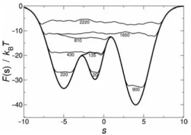
(18) Chapter 1 Theoretical Foundation. Topological approaches are based on a priori chemical knowledge of the system and its symmetry. This method was developed at the beginning by Wells [10] [11] [12] [13] and it is still used to define networks that correspond to real or hypothetical crystal structures. However, selecting the most reasonable crystal structure among all the possible topologies, which depends strongly on the interatomic interaction considered and the structure groups taken into account, is not easy. Using the concept of topological crystal structure representation, it is possible to consider all possible topologies and subsequently reach to those that might correspond to the given crystal structure. The analysis starts from a complete representation of the crystal structure, where all atoms and all possible interatomic interactions, even the weakest, are considered as nodes and edges on a graph, respectively. It is assumed that this representation contains all the information on the crystal. For a particular system, a three-step method for simplification is proposed to reach the desired partial representation [14]. Although the above methods have proven their usefulness and are still used, in one way or another, their use is conditioned to a previous knowledge of the system symmetry and empirical results. In order to obtain more unbiased results in the prediction of crystal structures, the abinitio computational approach has been fundamental, essentially because of the following two reasons among others [1]: - The computational approach allows to calculate explicitly the physical quantity desired (e. g. the energy) - Given the fact that no empirical information is used, the searching techniques can explore the whole energy landscape with virtually no bias and eventually provide unexpected results such as previously unknown crystal structures. The computational techniques developed so far consider the crystal structure prediction as an optimization problem, in which the aim is to find the energy landscape’s global minimum. To do that, these techniques seek deformations inside the energy landscape and follow them, trying to find the low energy regions, which are associated with dynamically stable structures. These low energy regions are usually close to each other, and they form energy funnels of different sizes and shapes, as shown in figure 1.2.. Page 5.

(19) Chapter 1 Theoretical Foundation. Figure 1.2. Energy landscape. It contains kinetics traps and energy barriers. Taken from [15].. Taking into account that in real chemical systems, there are only a few (sometimes even one) energy funnel, the efficiency of the searching can be significantly improved. Some of the techniques that use this fact are: Random Sampling, Simulated Annealing, Metadynamics, Molecular Dynamics and Evolutionary Algorithms. In the following sections we present and overview of these methods one by one.. RANDOM SAMPLING Random sampling is a stochastic method used to explore the energy surface of a system [16]. Eventually this technique was refined [17] [18] [19] [20] until it reached a wide accepted general procedure: given certain details of the system, e. g. the stoichiometry of a crystal or a protein sequence, the algorithm generates randomly the structure of the system, and by applying some local optimization algorithms, the total energy of a local minimum is calculated. This procedure is carried out until a satisfactory solution is achieved [21], as shown in figure 1.3. Page 6.

(20) Chapter 1 Theoretical Foundation. Figure 1.3. Simplified version of a Random Sampling algorithm.. Chris J. Pickard and Richard Needs have applied widely this technique in several crystal molecular systems and semiconductors using DFT, such as: SiH4 [22], CaC6 [23], AlH3 [24], H2O [25], hydrogen [26], nitrogen [27], iron [28] and lithium [29]. Some of these systems have up to 24 atoms per cell, but most of them contain less than 12 atoms per cell. Some studies have combined this technique with others [30] [31] [32]. Also, Random Sampling has been applied for study small organic molecules for comparative effects [33] [34].. SIMULATED ANNEALING The simulated annealing algorithm is mostly based on Monte Carlo Metropolis algorithm, which describes a random path at constant temperature, using an acceptance criterion. When the temperature is no longer constant in the algorithm, the simulated annealing method is obtained [35] [36]. While the temperature is decreasing, the variation in the random path will be, in average, lower due to the constant decrease of energy. At the end of the process, the system is. Page 7.

(21) Chapter 1 Theoretical Foundation. expected to reach the global energy minimum, but this depends on a well set up cooling process [37]. A simple way to understand the fundamentals of this algorithm is to imagine a hermetic box that contains an irregular surface inside and a sphere that is located at any point on that surface, as shown in figure 1.4.. Figure 1.4. Schematic representation of simulated annealing. Taken from [38].. The goal is to move the sphere to the lowest point of the surface inside the box. At the beginning of the process the system temperature is high and some perturbations are applied to make the sphere get the energy to jump easily the peaks of the surface. While the temperature is decreasing, the sphere finds harder to jump those peaks, so it is expected that at the end of the process the sphere will be located at the lowest point of the surface, or in a worse-case scenario in a region near to the lowest point [38].. MOLECULAR DYNAMICS Molecular dynamics is a technique that aims to calculate the equilibrium dynamical properties of an N body physical system at a given set of temperatures. Although the behavior of all the particles could be described by Quantum Mechanics, Molecular Dynamics assumes, in principle, that atomic nuclei obey the Classical Mechanics laws, In fact, it doesn’t take into account. Page 8.

(22) Chapter 1 Theoretical Foundation. relativity or Quantum Mechanics for the nuclei [39] and this approximation has worked properly for several materials [40]. However, when it’s necessary, semi-classical corrections can be applied to the desired system [41].. Figure 1.5. Particle trajectory in Molecular Dynamics simulation. Taken from [42].. Molecular Dynamics is based on determining the movement of the particles of the system resolving Newton’s laws of motion. To achieve this, numerical integration is used on every particle, step by step, during certain period of time. The description of the particle trajectory, as shown in figure 1.5, has been described using several algorithms [43], which are detailed in table 1.2. Table 1.2. Several algorithms used in Molecular Dynamics.. Page 9.

(23) Chapter 1 Theoretical Foundation. Ab-initio Molecular Dynamics has been widely developed by Michele Parrinello and Roberto Car, who made possible an efficient unification of this technique with Density Functional Theory, creating the Car – Parrinello algorithm [44] [45].. METADYNAMICS Metadynamics is an improvement on Molecular Dynamics which aims to reconstruct the free energy of complex systems using. artificial dynamics. Taking into account that the free energy. surface has many local minima separated by high barriers, the spontaneous transition from one local minimum to another is not easy to achieve. The algorithm first defines the dynamic variables (also called degrees of freedom) of the system inside a vector: ̃ = (ℎ11 , ℎ22 , ℎ33 , ℎ44 , ℎ55 , ℎ66 )𝑇 𝒉. (3). Following the generic metadynamic algorithm [46][26], the discrete dynamic of the system is defined:. ̃ 𝑡+1 = 𝒉 ̃ 𝑡 + 𝛿ℎ 𝒉. 𝝓𝑡 |𝝓𝑡 |. 𝑤ℎ𝑒𝑟𝑒: 𝝓𝑡 = −. ̃ ) = 𝐺(𝒉 ̃ ) + ∑ 𝑊𝑒 𝐺 𝑡 (𝒉. −. ̃ −𝒉 ̃ 𝑡′ | |𝒉 2𝛿ℎ2. 𝜕𝐺 𝑡 ̃ 𝜕𝒉. (4). 2. (5). 𝑡 ′ <𝑡. ̃ ) includes a Gaussian term that is added to each new point 𝒉 ̃ 𝑡′ in The Gibbs potential, 𝐺 𝑡 (𝒉 order to mark the points inside the free energy surface that have been already visited and avoid them in future iterations, by doing this the system is forced to leave one energy minimum while the simulation is going forward, due to the Gaussian contributions to the energy that are progressively filling the low potential regions allowing the system to go to other local minima and eventually covering the entire free energy surface. This process is shown in figure 1.6.. Page 10.

(24) Chapter 1 Theoretical Foundation. Figure 1.6. Schematic representation of the progressive filling of the underlying potential (thick line) by means of the Gaussian contributions deposited along the trajectory. The sum of the underlying potential and of the metadynamics bias is shown at different times (thin lines). Taken from [47].. EVOLUTIONARY ALGORITHMS This type of algorithm uses mechanisms inspired on biological evolution, such as reproduction, mutation, recombination and selection [48]. The possible solutions of the optimization problem are treated as individuals inside a population that evolves under the terms mentioned earlier and the quantity of individuals that will survive is determined by a fitness solution. The algorithm itself can be implemented as follows [4] [5]: first of all, an accurate representation of the problem must be chosen. The quality of this representation has a direct impact in the effectiveness of the algorithm. Once the representation is set up, the first generation is created and the quality of life of each individual is determined by the fitness function. The best individuals of this generation are selected as parents of the next generation. The offspring will be ruled by the same fitness function, and the best individuals will create the third generation. These steps will be repeated until the convergence criteria is achieved.. Page 11.

(25) Chapter 1 Theoretical Foundation. THE ELECTRONIC PROBLEM Matter can be described (in very simplistic terms) as a set of atoms that interact with each other, sometimes under the influence of an external field. This arrangement of particles may be in the gas or in a condensed phase, which in turn can be a solid, liquid or amorphous phase. Despite the multiple ensembles that can be formed, all these systems can be described as a set of atomic nuclei and electrons that interact among themselves under the influence of electrostatic forces. Therefore the Hamiltonian of such system can be expressed as: 𝑃. 𝑁. 𝐼=1. 𝑖=1. 𝑃. 𝑃. 𝑁. 𝑁. ℏ2 2 ℏ2 2 𝑒 2 𝑍𝐼 𝑍𝐽 𝑒2 1 ̂ ℋ = −∑ ∇𝐼 − ∑ ∇𝑖 + ∑ ∑ + ∑∑ 2𝑀𝐼 2𝑚 2 |𝑹𝐼 − 𝑹𝐽 | 2 |𝒓𝑖 − 𝒓𝑗 | 𝑃. 𝐼=1 𝐽≠𝐼. 𝑁. 2. − 𝑒 ∑∑ 𝐼=1 𝑖=1. 𝑍𝐼 |𝑹𝐼 − 𝒓𝑖 |. 𝑖=1 𝑗≠𝑖. (6). Where 𝑹 = {𝑹𝐼 , 𝐼 = 1 … 𝑃} and 𝒓 = {𝒓𝑖 , 𝑖 = 1 … 𝑁} are a set of P nuclear coordinates and N electronic coordinates. ZI and MI are the nuclear charges and masses respectively. The first and second term represent the kinetic energy of the P nuclei and the N electrons of the system. The third term represents the interaction between nuclei; this potential can be reduced to an additive constant when an approximation is used in order to resolve the electronic problem. The last two terms correspond to the interaction between electrons and the interaction between nuclei and electrons, respectively. Before continuing, there are some considerations about the Hamiltonian expressed in equation (6) that have to be taken into account: - The kinetic energy calculated in the first and second terms, and the motion of nuclei and electrons, are treated strictly in a non-relativistic way. - The definition of each term of the Hamiltonian implies that the nuclei are treated as point particles, characterized only by their mass, charge and magnetic moment. - The interaction between charged particles, calculated in the last three terms, is given by the instantaneous and spin-independent Coulomb interaction.. Page 12.

(26) Chapter 1 Theoretical Foundation. - The equation (6) shows a free-field system Hamiltonian. However, an electromagnetic field can be indicated when necessary, and this field can be either static or time-dependent. In principle, all the properties of this system can be derived by solving the time-independent Schrödinger equation: ̂ 𝜓𝑛 (𝑹, 𝒓) = 𝜀𝑛 𝜓𝑛 (𝑹, 𝒓) ℋ. (7). Where 𝜀𝑛 are the energy eigenvalues and 𝜓𝑛 (𝑹, 𝒓) are the eigenstates, or wave functions. Since the electrons are fermions, the wave function must be antisymmetric with respect to the exchange of the electronic coordinates r, and symmetric or antisymmetric with respect to the exchange of the nuclear coordinates R, having into account that different nuclear species are distinguishable but the statistics used for systems made only of one type of atom depends on the nuclear spin of it. However, in general this problem is practically impossible to solve analytically within the full quantum mechanics formalism: the system is a many-body system, where each particle position is described by three spatial coordinates. In addition, the Coulomb interaction is the result of pairwise terms, so the Schrödinger equation cannot be separated. As a result of this limitation, we have to deal in principle with a 3(P+N) degrees of freedom problem. Nevertheless, several approximations have been proposed and refined in order to reduce the complexity of the electronic problem, one such approximation is the Born-Oppenheimer Approximation.. BORN – OPPENHEIMER APPROXIMATION The first step towards the solution of equation (6) is to partially decouple the electronic and the nuclear motion. This can be achieved due to the difference between the electrons’ and nuclei’s time-scales. Inside the classical scheme and under typical conditions, the velocity of an electron is much larger than the proton’s, because the mass of the proton is approximately 1836 times larger than the. Page 13.

(27) Chapter 1 Theoretical Foundation. electron’s. Taking that into account, Max Born and J. Robert Oppenheimer proposed in 1927 a way to separate the nuclear motion from the electronic motion [49]. Every time the nuclei move, the electrons adjust their positions very fast; therefore their wave function is always adjusted to the nuclear wave function almost instantaneously. Then the equation (7) can be solved with a factorized wave function that contains a nuclear component and an electronic component of the form:. 𝜓(𝑹, 𝒓, 𝑡) = ∑ Θ𝑛 (𝑹, 𝑡)Φ𝑛 (𝑹, 𝒓). (8). 𝑛. Where Θ𝑛 (𝑹, 𝑡) are the wave functions that describe the evolution of the nuclear movement and Φ𝑛 (𝑹, 𝒓) are the electronic eigenstates. These terms satisfy the time-independent Schrödinger equation: ℎ̂𝑒 Φ𝑛 (𝑹, 𝒓) = 𝐸𝑛 (𝑹)Φ𝑛 (𝑹, 𝒓). (9). This equation represents a stationary eigenvalue problem for a given set of parameters R, which corresponds to the 3P nuclear coordinates and acts as a parameter of the equation. Therefore, the electronic problem has to be solved for a set of electronic positions r that depend on a particular nuclear configuration. Finally, the electronic Hamiltonian, according to the equation (6), is defined as follows: 𝑃. ̂ +∑ ℎ̂𝑒 = ℋ 𝐼=1. 𝑃. 𝑃. ℏ2 2 𝑒 2 𝑍𝐼 𝑍𝐽 ∇𝐼 − ∑ ∑ 2𝑀𝐼 2 |𝑹𝐼 − 𝑹𝐽 | 𝐼=1 𝐽≠𝐼. ̂ − 𝑇̂𝑛 − 𝑉̂𝑛𝑛 = 𝑇̂ + 𝑈 ̂𝑒𝑒 + 𝑉̂𝑒𝑛 ℎ̂𝑒 = ℋ. (10). Solving the time-independent Schrödinger equation will provide the key for understanding matter. However, in order to study the structure of matter, most of the time we only care about. Page 14.

(28) Chapter 1 Theoretical Foundation. the ground electronic states. This does not imply that excited states are less important2, but the complexity of the solution is higher than the one for ground states.. HARTREE AND HARTREE – FOCK APPROXIMATIONS Finding the ground state in an inhomogeneous system composed by N particles such as electrons, is one of the most important problems in the quantum many–body theory. Using the Dirac’s Notation3 and the electronic Hamiltonian defined in the equation (10), the ground state energy is given by: ̂𝑒𝑒 |Φ⟩ = ⟨Φ|𝑇̂|Φ⟩ + ⟨Φ|𝑉̂𝑒𝑥𝑡 |Φ⟩ + ⟨Φ|𝑈 ̂𝑒𝑒 |Φ⟩ 𝐸 = ⟨Φ|𝑇̂ + 𝑉̂𝑒𝑥𝑡 + 𝑈. (11). Where |Φ⟩ is the N-electron ground state wave function, 𝑇̂ is the kinetic energy operator, 𝑉̂𝑒𝑥𝑡 is a generalized form of the term 𝑉̂𝑒𝑛 (electron–nucleus interaction defined in equation (10)), that ̂𝑒𝑒 is corresponds to the interaction with fields that are external to the electronic system, and 𝑈 the electron-electron interaction. These terms can be written as follows:. 𝑇 = ⟨Φ|𝑇̂|Φ⟩ =. −ℏ2 ⟨Φ| ∑𝑁 𝑖=1 2𝑚. 𝑁. ∇2𝒊. −ℏ2 |Φ⟩ = ∑⟨Φ|∇2𝒊 |Φ⟩ 2𝑚 𝑖=1. 2. 𝑇=. −ℏ ∫[∇2𝒊 𝜌1 (𝒓, 𝒓′)]𝒓=𝒓′ 𝑑𝒓 2𝑚. (12) 𝑁. 𝑉𝑒𝑥𝑡 = ⟨Φ|𝑉̂𝑒𝑥𝑡 |Φ⟩ =. ⟨Φ| ∑𝑁 𝑖=1 𝑣𝑒𝑥𝑡 (𝒓𝑖 ) |Φ⟩. = ∑⟨Φ|𝑣𝑒𝑥𝑡 (𝒓𝑖 )|Φ⟩ 𝑖=1. = ∫[𝑣𝑒𝑥𝑡 (𝒓)𝜌1 (𝒓, 𝒓′ )]𝒓=𝒓′ 𝑑𝒓 𝑉𝑒𝑥𝑡 = ∫ 𝑣𝑒𝑥𝑡 (𝒓)𝜌(𝒓)𝑑𝒓. (13). Excited electronic states allow the study of phenomena like electronic transport, optical properties and photodissociation. 3 For more detailed information on Dirac’s Notation and Second Quantization, please remit to Appendix A. 2. Page 15.

(29) Chapter 1 Theoretical Foundation. 𝑁. 𝑈𝑒𝑒. 𝑁. 1 1 1 𝑁 1 ̂𝑒𝑒 |Φ⟩ = ⟨Φ| ∑𝑁 = ⟨Φ|𝑈 |Φ⟩ = ∑ ∑ ⟨Φ| |Φ⟩ 𝑖=1 ∑𝑗≠𝑖 2 2 |𝒓𝑖 − 𝒓𝑗 | |𝒓𝑖 − 𝒓𝑗 | 𝑖=1 𝑗≠𝑖. 1 𝜌(𝒓)𝜌(𝒓′) 𝑈𝑒𝑒 = ∬ 𝑑𝒓𝑑𝒓′ |𝒓 − 𝒓′| 2. (14). Introducing the two-body direct correlation, 𝑔(𝒓, 𝒓′ ), as: 𝜌2 (𝒓, 𝒓′ ) = 𝜌(𝒓)𝜌(𝒓′ )𝑔(𝒓, 𝒓′ ). (15). We have that for an uncorrelated system 𝑔(𝒓, 𝒓′ ) = 1, therefore the electron-electron interaction can be re-written as: 1 𝜌2 (𝒓, 𝒓′ ) 𝑈𝑒𝑒 = ∬ 𝑑𝒓𝑑𝒓′ |𝒓 − 𝒓′| 2. (16). In this term the two-body interaction is reduced to a classical electrostatic interaction. This is known as the Hartree Approximation. In order to build a more realistic model, the effect of the repulsion force produced by two electrons that are located at positions r and r’, respectively, and are close to each other, has to be taken into account. This can be solved adding a term that includes both exchange and correlation effects: 1 𝜌2 (𝒓, 𝒓′ ) 1 𝜌2 (𝒓, 𝒓′ ) [𝑔(𝒓, 𝒓′ ) − 1]𝑑𝒓𝑑𝒓′ 𝑈𝑒𝑒 = ∬ 𝑑𝒓𝑑𝒓′ + ∬ |𝒓 − 𝒓′| |𝒓 − 𝒓′| 2 2. (17). In the Hartree approximation the electrons are treated as distinguishable particles. However, electrons are indistinguishable spin-1/2 fermions, so, their many-body wave function has to be anti-symmetric in order to obey Pauli’s Exclusion Principle, but Hartree’s approximation doesn’t take this into account, as a consequence, the model that describes the electronic part of the atomic system is incomplete.. Page 16.

(30) Chapter 1 Theoretical Foundation. Pauli’s Exclusion Principle can be easily introduced by proposing an anti-symmetrized manybody wave function in the form of a Slater determinant. Once we have done this, we are in the Hartree-Fock scheme: 𝜑1 (1) 𝜑2 (1) 1 𝜑1 (2) 𝜑2 (2) Φ𝐻𝐹 (𝒙1 , 𝒙2 , … , 𝒙𝑁 ) = [ ⋮ ⋮ √𝑁! 𝜑1 (𝑁) 𝜑2 (𝑁). ⋯ 𝜑𝑁 (1) ⋯ 𝜑𝑁 (2) ] ⋱ ⋮ ⋯ 𝜑𝑁 (𝑁). (18). Where 𝜑𝑖 (𝑗) is the i-th one-electron spin orbital, which is composed of spatial and spin components that are condensed in a single variable (𝒙𝑗 = (𝒓𝑗 , 𝜎𝑗 ) and is the result of Hartree’s assumption that the many-electron wave function can be expressed as a product of one-electron orbitals: 𝑁. Φ(𝒓) = ∏ 𝜑𝑖 (𝒓𝑖 ). (19). 𝑖=1. Once we have set the wave function, we are able to determine the Hartree-Fock energy by calculating the one-electron contribution: 𝑁. 𝐸. (1). = ∫Φ. ∗ (𝒓). 𝑁. (∑ ℎ̂𝑖 (𝑖)) Φ(𝒓)𝑑𝒓 = ∑ 𝐸𝑖𝑖 𝑖=1. 𝑤ℎ𝑒𝑟𝑒: ℎ̂𝑖 (𝑖) = −. (20). 𝑖=1 2. ℏ 2 ∇ + 𝑣𝑒𝑥𝑡 (𝑹, 𝒓𝑖 ) 2𝑚 𝒓𝑖. (21). And the two-electron contribution to the energy: 𝑁. 𝐸. (2). = ∫Φ. ∗ (𝒓). 𝑁. 𝑁. 𝑁. 1 1 ( ∑ ∑ 𝑣̂2 (𝑖, 𝑗)) Φ(𝒓)𝑑𝒓 = ∑ ∑(𝐽𝑖𝑗 − 𝐾𝑖𝑗 ) 2 2 𝑖=1 𝑗≠𝑖. 𝑤ℎ𝑒𝑟𝑒: 𝑣̂2 (𝑖, 𝑗) =. (22). 𝑖=1 𝑗≠𝑖. 1 |𝒓𝑖 − 𝒓𝑗′ |. (23). Where the Coulomb and exchange integrals are defined as:. Page 17.

(31) Chapter 1 Theoretical Foundation. 𝐽𝑖𝑗 = ∬ 𝜑 ∗ (𝑖)𝜑 ∗ (𝑗)𝑣̂2 (𝑖, 𝑗)𝜑(𝑖)𝜑(𝑗)𝑑𝒙𝑖 𝑑𝒙𝑗. (24). 𝐾𝑖𝑗 = ∬ 𝜑 ∗ (𝑖)𝜑 ∗ (𝑗)𝑣̂2 (𝑖, 𝑗)𝜑(𝑗)𝜑(𝑖)𝑑𝒙𝑖 𝑑𝒙𝑗. (25). Finally the Hartree-Fock energy is: 𝑁. 𝐸𝐻𝐹 = 𝐸. (1). +𝐸. (2). 𝑁. 𝑁. 1 = ∑ 𝐸𝑖𝑖 + ∑ ∑(𝐽𝑖𝑗 − 𝐾𝑖𝑗 ) 2 𝑖=1. (26). 𝑖=1 𝑗≠𝑖. The Hartree-Fock approximation, or Self-Consistent Field (SCF), is described in the following algorithm:. Figure 1.7. Self-Consistent Field (SCF) algorithm. Adapted from [50].. Page 18.

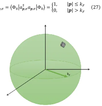
(32) Chapter 1 Theoretical Foundation. Even when the determinant satisfies Pauli’s Exclusion Principle, the wave function doesn’t contain the correlation term that results from the interaction between electrons, or Coulomb interaction, but this can be solved by constructing the wave function Φ𝐻𝐹 (𝒙1 , 𝒙2 , … , 𝒙𝑁 ) with more than one determinant in what is known as a Configuration Interaction (CI) scheme.. THOMAS – FERMI THEORY By the same time when Hartree and Fock proposed their approach, L.H. Thomas and Enrico Fermi proposed a method for calculating the energy of an electronic system that depended only on the electronic density. Fermi said that in the ground state of a gas of N free electrons, |Φ0 ⟩, the particle states with wave number up to 𝑘𝐹 were occupied and lied within the Fermi sphere, as showed in figure 1.8. The zero temperature expectation value of the particle number operator in the momentum space is determined as: 1, † 𝑛𝒑,𝜎 = ⟨Φ0 |𝑎𝒑,𝜎 𝑎𝒑,𝜎 |Φ0 ⟩ = { 0,. |𝒑| ≤ 𝑘𝐹 |𝒑| > 𝑘𝐹. (27). 2𝜋 3. Figure 1.8. The Fermi sphere with an infinitesimal volume of 𝑑𝒑3 in the real space, or ( ) in the K-space. 𝐿. Page 19.

(33) Chapter 1 Theoretical Foundation. The total particle number can be calculated as: 𝑘𝐹. 𝑁 = ∑ 𝑛𝒑,𝜎 𝒑,𝜎. 𝑘𝐹. 𝑑𝒑3 𝐿3 𝑉 4𝜋𝑘𝐹 3 𝑉𝑘𝐹 3 3 = 2 ∑ 1 = 2∫ = ∫ 𝑑𝒑 = 3 = (2𝜋⁄𝐿)3 4𝜋 3 4𝜋 3 3𝜋 2 𝒑≤𝑘𝐹. 0. (28). 0. Then, the mean particle density is: 𝑁 𝑘𝐹 3 𝜌= = 2 𝑉 3𝜋. (29). Where 𝑘𝐹 is the Fermi wave vector, the Fermi momentum is defined as 𝑝𝐹 = ℏ𝑘𝐹 , and the Fermi energy, that is the energy of the top-most filled level in the ground state of the N free-electron system, is defined as 𝜖𝐹 =. (ℏ𝑘𝐹 )2 2𝑚. . Now, the mean particle density 𝜌 in terms of the Fermi energy. is: 3⁄ 2. 1 2𝑚 𝜌 = 2( ) 3𝜋 ℏ. 𝜖𝐹. 3⁄ 2. (30). Fermi proposed an expression for the total electronic energy for an inhomogeneous system from the definition of kinetic, exchange and correlation contributions in the homogeneous gas:. 𝐸𝛼 [𝜌] = ∫ 𝜌(𝒓)𝜀𝛼 [𝜌(𝒓)]𝑑𝒓. (31). Where 𝜀𝛼 contains the kinetic, exchange and correlation energy density contributions, calculated locally at every point in space. This was the first attempt to obtain a Local Density Approximation (LDA) to the electronic problem. As a remark, in the original Thomas-Fermi method, they neglected the exchange and correlation between electrons. The local approximation for exchange was introduced later by Dirac. Therefore, with the inclusion of that term the theory is now called Thomas-Fermi-Dirac. Then, the energy functional for an electron in an external potential 𝑣𝑒𝑥𝑡 (𝒓) is defined as:. Page 20.

(34) Chapter 1 Theoretical Foundation. 𝐸𝑇𝐹𝐷 [𝜌] = 𝐶1 ∫ 𝜌(𝒓). 5⁄ 3 𝑑𝒓. + 𝐸𝐶 [𝜌]. 1 𝜌(𝒓)𝜌(𝒓′) 4 + ∫ 𝜌(𝒓)𝑣𝑒𝑥𝑡 (𝒓)𝑑𝒓 + ∬ 𝑑𝒓𝑑𝒓′ + 𝐶2 ∫ 𝜌(𝒓) ⁄3 𝑑𝒓 |𝒓 − 𝒓′| 2. (32). The first term is the LDA kinetic energy with 𝐶1 = 3 3. 1⁄ 3. the local exchange with 𝐶2 = − 4 (𝜋). 3 10. (3𝜋 2 ). 2⁄ 3. = 2.871𝑎. 𝑢.; the fourth term is. = 0.739𝑎. 𝑢.; and the last term is the correlation:. 𝐸𝐶 [𝜌] = −0.056 ∫. 𝜌(𝒓) 0.079 + 𝜌(𝒓). 1⁄ 𝑑𝒓 3. (33). It is easy to realize that equation (32) only depends on the electronic density, that’s the reason why it is said that this is a functional of the density. Nevertheless, the formal mathematical framework for this type of functional was developed by Hohenberg and Kohn more than thirty years after Thomas, Fermi and Dirac developed their idea of a density functional.. HOHENBERG – KOHN THEOREMS The approach of Hohenberg and Kohn was to formulate the density functional theory as an exact theory of many-body systems. Their theorems can be applied to any system of interacting particles in an external potential 𝑣𝑒𝑥𝑡 (𝒓). They also established a set of relations that are represented as:. Figure 1.9. Schematic representation of Hohenberg-Kohn Theorem. Adapted from [51].. Page 21.

(35) Chapter 1 Theoretical Foundation. Where the thin arrows represent the usual solution of the Schrödinger equation, where the potential 𝑣𝑒𝑥𝑡 (𝒓) determines all the states of the system Φ𝑖 ({𝒓}), including the ground state Φ0 (𝒓) and the density ground state 𝜌0 (𝒓). The Hohenberg-Kohn theorems complete the cycle. The following two theorems [51] are the foundation of the Density Functional Theory: Theorem I:. For any system of interacting particles in an external potential 𝑣𝑒𝑥𝑡 (𝒓), the potential 𝑣𝑒𝑥𝑡 (𝒓) is determined uniquely, except for a constant, by the ground state particle density 𝜌0 (𝒓). Proof: 1 (𝒓) 2 (𝒓), Suppose that we have two different external potentials 𝑣𝑒𝑥𝑡 and 𝑣𝑒𝑥𝑡. which differ by more than a constant. Each potential leads to a different ̂1 and ̂ Hamiltonian 𝐻 𝐻 2 , which have different ground state wave function Φ1 and Φ2 , which are hypothesized to have the same ground state density 𝜌0 (𝒓). ̂1 , we have: Since Φ2 is not the ground state of 𝐻 ̂1 |Φ1 ⟩ < ⟨Φ2 |𝐻 ̂1 |Φ2 ⟩ 𝐸1 = ⟨Φ1 |𝐻 ̂1 |Φ2 ⟩ can be rewritten as: ⟨Φ2 |𝐻 ̂1 |Φ2 ⟩ = ⟨Φ2 |𝐻 ̂ 2 |Φ2 ⟩ + ⟨Φ2 |𝐻 ̂1 − 𝐻 ̂ 2 |Φ2 ⟩ ⟨Φ2 |𝐻 1 (𝒓) 2 (𝒓)]𝑑𝒓 = 𝐸 2 + ∫ 𝜌0 (𝒓)[𝑣𝑒𝑥𝑡 − 𝑣𝑒𝑥𝑡. Replacing:. 1 (𝒓) 2 (𝒓)]𝑑𝒓 𝐸1 < 𝐸 2 + ∫ 𝜌0 (𝒓)[𝑣𝑒𝑥𝑡 − 𝑣𝑒𝑥𝑡. Making the same procedure for 𝐸 2 we have:. Page 22.

(36) Chapter 1 Theoretical Foundation. 2 (𝒓) 1 (𝒓)]𝑑𝒓 𝐸 2 < 𝐸1 + ∫ 𝜌0 (𝒓)[𝑣𝑒𝑥𝑡 − 𝑣𝑒𝑥𝑡 1 (𝒓) 2 (𝒓)]𝑑𝒓 = 𝐸1 − ∫ 𝜌0 (𝒓)[𝑣𝑒𝑥𝑡 − 𝑣𝑒𝑥𝑡. Adding the two inequalities: 𝐸1 + 𝐸 2 < 𝐸1 + 𝐸 2 This result is absurd, therefore is not possible that two different potentials can lead to the same ground density. Corollary I:. Since the Hamiltonian is thus fully determined, except for a. constant shift of the energy, it follows that the many-body wave functions for all states (ground and excited) are determined. Therefore, all the properties of the system are completely determined given only the ground state density 𝜌0 (𝒓). Theorem II:. An universal functional for the energy 𝐸[𝜌] in terms of the density 𝜌(𝒓) can be defined, valid for any external potential 𝑣𝑒𝑥𝑡 (𝒓). For any particular 𝑣𝑒𝑥𝑡 (𝒓), the exact ground state energy of the system is the global minimum value of this functional and the density 𝜌(𝒓) that minimizes the functional is the exact ground state 𝜌0 (𝒓). Proof: Since all properties of the system are uniquely determined if 𝜌(𝒓) is specified, then the total energy functional can be expressed as:. 𝐸𝐻𝐾 [𝜌] = 𝑇[𝜌] + 𝑈𝑒𝑒 [𝜌] + ∫ 𝜌(𝒓)𝑣𝑒𝑥𝑡 (𝒓)𝑑𝒓 = 𝐹𝐻𝐾 [𝜌] + ∫ 𝜌(𝒓)𝑣𝑒𝑥𝑡 (𝒓)𝑑𝒓. Let’s consider a system with ground state density 𝜌01 (𝒓), which corresponds to the 1 (𝒓). potential 𝑣𝑒𝑥𝑡 The Hohenberg-Kohn functional (𝐹𝐻𝐾 [𝜌]) is equal to the. Page 23.

(37) Chapter 1 Theoretical Foundation. expectation value of the Hamiltonian in the unique ground state which has wave function Φ1 . ̂1 |Φ1 ⟩ 𝐸1 = ⟨Φ1 |𝐻 Now, let’s consider a different density 𝜌02 (𝒓) which corresponds to a different wave function Φ2 . Then: ̂1 |Φ2 ⟩ > ⟨Φ1 |𝐻 ̂1 |Φ1 ⟩ = 𝐸1 𝐸 2 = ⟨Φ2 |𝐻 Therefore the energy evaluated by 𝐹𝐻𝐾 [𝜌] is greater for any 𝜌(𝒓) different from the ground state density 𝜌0 (𝒓). Corollary II:. The functional 𝐸[𝜌] alone is sufficient to determine the exact. ground state energy and density. In general, excited states of the electrons must be determined by other means. In conclusion, 𝐹𝐻𝐾 [𝜌] is an universal functional which does not depend explicitly on the external potential, it depends only on the electronic density, and by knowing it we can know the solution of the full many-body Schrödinger equation.. KOHN – SHAM METHOD Nowadays, Density Functional Theory is one of the most used techniques for electronic structure calculations. This is because of the practical approach proposed by Kohn and Sham [52]. One good strategy, in order to solve the electronic problem, is to separate the different energy contributions. For instance, as discussed before, the separation of the Hartree term from the exchange and correlation contributions. Therefore, the electron-electron interaction is divided into three terms: Hartree, exchange, and correlation. The Hartree term is just the classical electrostatic energy, which is exact. The exchange term can be calculated exactly inside the Hartree-Fock scheme, however, due to computational reasons most of the time it is an. Page 24.

(38) Chapter 1 Theoretical Foundation. approximate term. Finally, the correlation term, the smallest contribution to the energy, contains all of the unknowns about the many body problem. The Kohn-Sham method reuses the idea of separation of elements: they replace the original many-body problem with a different auxiliary system that is easier to solve. The key of their idea is to assume that the ground state density of the interacting system is equal to the density of some chosen non-interacting system. As a consequence, a new set of particle-independent equations is defined for the non-interacting system and once they are solved we can find the ground state density and energy of the original system, with an error margin reduced to the approximation used in the exchange-correlation functional. At this point, the main problem is with the kinetic energy term 𝑇 = ⟨Φ|𝑇̂|Φ⟩, because its explicit expression in terms of the electronic density is unknown. In the Thomas-Fermi scheme, the kinetic energy is calculated locally, but this approach introduces an error into the model, given the nonlocal nature of this operator. Kohn and Sham realized that a system of non-interacting electrons is exactly described by an anti-symmetrized wave function of the Slater determinant type, made of one-electron orbitals. Then, the ground state density matrix 𝜌1 (𝒓, 𝒓′) is given by: ∞. 𝜌1 (𝒓, 𝒓′) = ∑ 𝑓𝑖 𝜑𝑖 (𝒓)𝜑𝑖∗ (𝒓′). (34). 𝑖=1. Where 𝜑𝑖 (𝒓) are the one-electron orbitals and 𝑓𝑖 are the occupation numbers corresponding to those orbitals. Then, the exact expression of the kinetic energy of non-interacting electrons can be set as: ∞. ℏ2 𝑇=− ∑ 𝑓𝑖 ⟨𝜑𝑖 |∇2 |𝜑𝑖 ⟩ 2𝑚. (35). 𝑖=1. Nevertheless, this expression is not the exact kinetic energy of the interacting system. The missing part is due to fact that the true many-body wave function is not a Slater determinant, therefore. Page 25.

(39) Chapter 1 Theoretical Foundation. there is a correlation contribution to the kinetic energy that is not taken into account and must be included in the correlation term. For now on, the equations defined here are in the equivalent non-interacting scheme. The noninteracting system made of N electrons and density 𝜌(𝒓) is described by the Hamiltonian: 𝑁. ̂𝑅 = ∑ [− ℋ 𝑖=1. ℏ2 2 ∇ + 𝑣𝑅 (𝒓𝑖 )] 2𝑚 𝑖. (36). ̂𝑅 equals 𝜌(𝒓). If Where 𝑣𝑅 (𝒓) is the reference potential in which the ground state density of ℋ that's so, the equivalence between the ground state energy and the energy of the interacting system is ensured by Hohenberg-Kohn's Theorem. Given the nature of the electrons, the occupation number of each orbital is 2, where the total number of electrons is 𝑁 = 𝑁 ↑ + 𝑁 ↓ and 𝑁𝑆 = 𝑁⁄2 is the number of orbitals with double occupancy. With these considerations, the density reads: 𝑁𝑆. 𝜌(𝒓) = ∑ ∑|𝜑𝑖𝜎 (𝒓)|2. (37). 𝜎 𝑖=1. The kinetic energy term is: 𝑁𝑆. 𝑁𝑆. ℏ2 ℏ2 𝑇𝑅 [𝜌] = − ∑ ∑⟨𝜑𝑖𝜎 |∇2 |𝜑𝑖𝜎 ⟩ = − ∑ ∑|∇2 𝜑𝑖𝜎 (𝒓)|2 2𝑚 2𝑚 𝜎 𝑖=1. (38). 𝜎 𝑖=1. And the Hartree term can be expressed as: 1 𝜌(𝒓)𝜌(𝒓′) 𝐸𝐻𝑎𝑟𝑡𝑟𝑒𝑒 [𝜌] = ∬ 𝑑𝒓𝑑𝒓′ |𝒓 − 𝒓′| 2. (39). Page 26.

(40) Chapter 1 Theoretical Foundation. Now, the universal density functional can be rewritten as: 𝐹[𝜌] = 𝑇𝑅 [𝜌] + 𝐸𝐻𝑎𝑟𝑡𝑟𝑒𝑒 [𝜌] + 𝐸̃𝑋𝐶 [𝜌] 𝑁𝑆. ℏ2 1 𝜌(𝒓)𝜌(𝒓′ ) 𝐹[𝜌] = − 𝑑𝒓𝑑𝒓′ + 𝐸̃𝑋𝐶 [𝜌] ∑ ∑|∇2 𝜑𝑖𝜎 (𝒓)|2 + ∬ |𝒓 − 𝒓′ | 2𝑚 2. (40). 𝜎 𝑖=1. The term 𝐸̃𝑋𝐶 [𝜌] does not only contain the exchange and correlation energy defined in equation 17, but also takes into account the kinetic correlation ignored in 𝑇𝑅 [𝜌]. Finally, we get the total energy functional:. 𝐸𝑣 [𝜌] = 𝐸𝐾𝑆 [𝜌] = 𝐹[𝜌] + ∫ 𝜌(𝒓)𝑣𝑒𝑥𝑡 (𝒓)𝑑𝒓 = 𝑇𝑅 [𝜌] + 𝐸𝐻𝑎𝑟𝑡𝑟𝑒𝑒 [𝜌] + 𝐸̃𝑋𝐶 [𝜌] + ∫ 𝜌(𝒓)𝑣𝑒𝑥𝑡 (𝒓)𝑑𝒓. (41). If the universal 𝐸̃𝑋𝐶 [𝜌] was known, then the exact ground state energy and density of the manybody problem could be found by solving the Kohn-Sham equations for a non-interacting system.. EXCHANGE AND CORRELATION IN DFT In order to solve the electronic problem, the strategy used was to separate the total energy into a number of different contributions: 𝐸[𝜌] = 𝑇𝑅 + 𝑣𝑒𝑥𝑡 + 𝐸𝐻 + 𝐸𝑋 + 𝐸̃𝐶. (42). In order of appearance there are: non-interacting kinetic energy, the interaction of the electrons with an external field, the classical electron-electron interaction, the exchange energy, and the coupling constant averaged correlation term.. Page 27.

(41) Chapter 1 Theoretical Foundation. This correlation energy is the central query. For instance, the exchange energy, as defined in equation 25 is very accurate: this calculation demands a lot of computer resources and usually several approximations are used in order to estimate its value, even when some error is introduced in the calculation. However, there isn’t an expression for the correlation energy with a level of accuracy comparable to that of the exchange energy. One way to address this issue is to consider the exchange and the correlation energy contributions, not independently, but as a sum of both terms 𝐸𝑋 + 𝐸̃𝐶 . The idea is now to find an approximation for both exchange and correlation, where they can be treated in a similar way. As seen before, one of the starting points for these approaches is the homogeneous gas and some approximations have been developed so far [53] [54] [55].. Local Density Approximation – LDA Local Density Approximation (LDA) was first formally introduced by Kohn and Sham [52], however the idea was used by Thomas, Fermi and Dirac in their theory. Basically LDA approach is to consider the inhomogeneous electronic system as a local homogeneous electron gas in which the exchange-correlation hole for this system is very accurate. The local energy is calculated at every point r with electronic density 𝜌(𝒓). Therefore, the exchange-correlation energy can be written in terms of the average energy 𝐿𝐷𝐴 [𝜌]: density 𝜖̃𝑋𝐶. 𝐿𝐷𝐴 [𝜌] 𝐿𝐷𝐴 [𝜌(𝒓)]𝑑𝒓 𝐸̃𝑋𝐶 = ∫ 𝜌(𝒓)𝜖̃𝑋𝐶. (43). 𝐿𝐷𝐴 (𝒓, 1 𝜌̃𝑋𝐶 𝒓′) ∫ 𝑑𝒓′ |𝒓 − 𝒓′| 2. (44). With. 𝐿𝐷𝐴 [𝜌(𝒓)] 𝜖̃𝑋𝐶 =. 𝐿𝐷𝐴 (𝒓, Where 𝜌̃𝑋𝐶 𝒓′) is the exchange-correlation hole and is defined as:. Page 28.

(42) Chapter 1 Theoretical Foundation. 𝐿𝐷𝐴 (𝒓, 𝜌̃𝑋𝐶 𝒓′) = 𝜌(𝒓){𝑔̃ℎ [|𝒓 − 𝒓′|, 𝜌(𝒓) ] − 1}. (45). With 𝑔̃ℎ [|𝒓 − 𝒓′|, 𝜌(𝒓) ] as the pair correlation function of the homogeneous gas. In practice the 𝐿𝐷𝐴 [𝜌] exchange-correlation energy is calculated according to equation 43 but using 𝜖̃𝑋𝐶 =. 𝜖𝑋𝐿𝐷𝐴 [𝜌] + 𝜖̃𝐶𝐿𝐷𝐴 [𝜌] as illustrated in table 1.3. Table 1.3. Expressions used to calculate the exchange-correlation energy in LDA. Adapted from [56].. [57] [58] [59]. As a final remark, the main limitations of LDA are [56]: - The inhomogeneities in the electronic density are not taken into account. - The self-interaction present in the Hartree term is not completely cancelled by the LDA exchange-correlation term. - LDA does not include non-local exchange and correlation effects. - Strong local correlation effects cannot be reproduced.. Generalized Gradient Approximation – GGA The Generalized Gradient Approximations (GGAs) were the way to try to solve LDA’s issues, especially regarding the inhomogeneities in the electronic densities. These approximations. Page 29.

(43) Chapter 1 Theoretical Foundation. propose an expansion of the density in terms of the gradient and other higher order derivatives, this expansion leads to the following exchange-correlation energy:. 𝐸𝑋𝐶 [𝜌] = ∫ 𝜌(𝒓)𝜀𝑋𝐶 [𝜌(𝒓)]𝐹𝑋𝐶 [𝜌(𝒓), ∇𝜌(𝒓), ∇2 𝜌(𝒓), … ] 𝑑𝒓. (46). Where 𝐹𝑋𝐶 is a factor that modifies the LDA expression, according to the variation of the density in the vicinity of one specific point. As a consequence, the energy is not calculated locally, but semi-locally. However, this approach is deficient when non-local effects have to be taken into account. The second order gradient expansion of the exchange energy correspond to an expression of the type:. 𝐸𝑋𝐶 [𝜌] =. 4 ∫ 𝐴𝑋𝐶 [𝜌(𝒓)]𝜌(𝒓) ⁄3 𝑑𝒓. +∫. 𝐶𝑋𝐶 [𝜌(𝒓)]|∇𝜌(𝒓)|2 𝜌(𝒓). 4⁄ 3. 𝑑𝒓. (47). Nevertheless, each term of the gradient expansion must be addressed very carefully, because some of them tend to violate at least one of the exact conditions required for the exchange and correlation holes, such as the normalization condition, the negativity of the exchange density or the self-interaction cancellation [56]. With these limitations in mind, there are two approaches to obtain GGAs: - The first one is to obtain the GGA via theoretical methods, where the coefficients are set up in such a way that the exact results of certain known parameters can be reproduced, like sum rules and long-range decay. - The second method is to fit the parameters in order to reproduce a set of experimental results. Typical parameters are formation energies, thermochemical data and structural parameters. Several gradient expansions have been proposed, mostly between the 80’s and mid 90’s. Three of the most used are summarized in table 1.4.. Page 30.

(44) Chapter 1 Theoretical Foundation. Table 1.4. Summary of several GGA functionals. Adapted from [56].. [60] [61] [62] [63]. The development of several GGAs marked an improvement over LDA in different aspects such as binding energies, atomic energies, bond lengths and angles. However, there are some other features that need to be enhanced [56]: - LDA describes better semiconductors than GGA. - The improvement of GGA over LDA for 4d – 5d transition metals and the gap energy is either not clear or not substantial in several cases. - GGA does not satisfy some known asymptotic behaviors, e. g. isolated atoms. - GGA functionals still do not compensate satisfactorily the self-interaction present in the Hartree term.. PSEUDOPOTENTIALS AND BASIS SETS Since the early stages of quantum mechanics, the solution of the many-body quantum problem is the main mathematical problem in electronic structure theory. The two main methodologies. Page 31.

(45) Chapter 1 Theoretical Foundation. proposed to address this problem, Hartree-Fock and Kohn-Sham, provide a tractable way to deal with this problem, but they are approximates schemes. The solution either of the Hartree-Fock or Kohn-Sham equations, regardless their approximated nature, requires two important choices [56]: - How to treat the electron-nuclear interaction. - Find a mathematical way to represent the single particle orbitals. Pseudopotentials The electron-nuclear interaction is given by the Coulomb potential defined as: 𝑃. 𝑁. 2. 𝑣𝑒𝑥𝑡 (𝒓) = −𝑒 ∑ ∑ 𝐼=1 𝑖=1. 𝑍𝐼 |𝑹𝐼 − 𝒓𝑖 |. (48). However, and as a manner of speak, there’s exist a distinction between three different classes of electrons4: Core electrons: they are tightly bound to the nuclei and are not involved in chemical bonding. Also they can be treated as frozen orbitals. Valence electrons: they are extended and participate actively in chemical bonding. Semi-core electrons: usually, they do not contribute directly to chemical bonding, due to their localized nature. However, they are close enough in energy to the valence states to feel the presence of the environment, therefore they cannot be treated as frozen orbitals. Since the core electrons are not fundamental for the description of the chemical bonding, it is possible to replace the charge of the atomic nuclei, which is treated point-like, with an effective nucleus charge of: 𝑍𝑣 = 𝑍 − 𝑍𝑐𝑜𝑟𝑒. (49). All electrons are the same, but this language abuse is used to indicate single-particle electronic states rather than electrons themselves. 4. Page 32.

(46) Chapter 1 Theoretical Foundation. Where 𝑍𝑐𝑜𝑟𝑒 is the charge associated to the core electrons. This effective core potential, or pseudopotential, represents the nucleus with its core electrons and it reduces significantly the number of degrees of freedom of the electron gas because the number of electrons treated explicitly is smaller, thus the number of required electronic states and the size of the basis set is also reduced. When the valence wave functions inside the core region can be neglected, these can be replaced with a smooth, nodeless pseudo-wave function as shown in figure 1.10:. Figure 1.10. Schematic illustration of all-electron (solid lines) and pseudoelectron (dashed lines) potentials and their corresponding wave functions. The radius at which all-electron and pseudoelectron values match is designated rc. Taken from [64].. The pseudopotentials have to be constructed very carefully in order to reproduce accurately the bonding properties of the all-electron potential, but maintaining the nodeless shape inside the core radius 𝑟𝑠 , and the construction is described in figure 1.11.. Page 33.

(47) Chapter 1 Theoretical Foundation. Figure 1.11. Flow chart describing the construction of an ionic pseudopotential for an atom. Taken from [64].. Finally, the most used pseudopotentials are non-conserving [65] [66] [67] [68] [69] and ultrasoft [70].. Basis Sets In order to solve the electronic problem in practice, it is necessary to find a mathematical representation for the one-electron orbitals. One possibility is to represent them in real space using a three-dimensional grid and then solve the partial differential equations using finite differences. Since the beginning of quantum mechanics, several basis sets have been developed for the Hilbert space based on the general characteristics and specific features of the system under study. Nowadays, the representation of the Kohn-Sham orbitals can be classified into four groups [56]:. Page 34.

(48) Chapter 1 Theoretical Foundation. - Extended basis sets: they are delocalized basis functions, either centered at the nuclear position or independent of them. Their most important feature is that they cover the whole space, therefore they are mostly used for condensed phases like solids and liquids. - Localized basis sets: as the name says, they are localized mainly at the atomic positions, but they can be centered in bonds. They are mostly used for molecular systems. - Mixed basis sets: they combine features from the extended and localized basis sets. However, their weakest point is the amount of technical issues when implemented. - Augmented basis sets: they are atomic like wave functions that augment and extended or localized basis set in spherical regions around the nuclei. The main feature is their high level of accuracy, but, from the technical point of view, they are much more complicated to implement. In this work we will be dealing mainly with a basis set of the extended type, i.e. plane waves.. REFERENCES [1] A. Oganov, «Introduction: Crystal Structure Prediction, a Formidable Problem,» from Modern Methods of Crystal Structure Prediction, New York, WILEY-VCH Verlag & Co. KGaA, 2011, pp. xi - xxi. [2] J. Maddox, «Crystals from first principles,» Nature, vol. 335, nº 6187, p. 201, 1988. [3] P. Erk, «Crystal Design,» de Crystal Engineering: From Molecules and Crystals to Materials, Springer Netherlands, 1999, pp. 143 - 161. [4] A. R. Oganov and C. Glass, «Crystal structure prediction using ab initio evolutionary techniques: Principles and applications,» Journal of Chemical Physics, vol. 124, nº 24, p. 244704, 2006. [5] C. W. Glass, A. R. Oganov and N. Hansen, «USPEX—Evolutionary crystal structure prediction. Computer Physics Communications,» Computer Physics Communications, vol. 175, nº 11 - 12, pp. 713 - 720, 2006. [6] G. N. Lewis, «The atom and the molecule,» Journal of the American Chemical Society, vol. 38, nº 4, pp. 762 - 785, 1916. [7] L. Pauling, «The Principles Determining the Structure of Complex Ionic Crystals,» Journal of the American Chemical Society, vol. 51, nº 4, pp. 10010 - 1026, 1929.. Page 35.

(49) Chapter 1 Theoretical Foundation. [8] I. D. Brown, «Bond valences—a simple structural model for inorganic chemistry,» Chemical Society Reviews, vol. 7, nº 3, pp. 359 - 376, 1978. [9] I. D. Brown, The Chemical Bond in Inorganic Chemistry: The Bond Valence Model, New York: OUP Oxford, 2006. [10] A. F. Wells, «The geometrical basis of crystal chemistry. Part 1,» Acta Crystallographica, vol. 7, nº 8 - 9, pp. 535 -544, 1954. [11] A. F. Wells, «The geometrical basis of crystal chemistry. Part 2,» Acta Crystallographica, vol. 7, nº 8 - 9, pp. 545 - 554, 1954. [12] A. F. Wells, «The geometrical basis of crystal chemistry. Part 3,» Acta Crystallographica, vol. 7, nº 12, pp. 842 - 848, 1954. [13] A. F. Wells, «The geometrical basis of crystal chemistry. Part 4,» Acta Crystallographica, vol. 7, nº 12, pp. 849 - 853, 1954. [14] V. A. Blatov, «A method for hierarchical comparative analysis of crystal structures,» Acta Crystallographica Section A, vol. 62, nº 5, pp. 356 - 364, 2006. [15] K. A. Dill and H. S. Chan, «From Levinthal to pathways to funnels,» Nature Structural Biology, vol. 4, nº 1, pp. 10 - 19, 1997. [16] R. L. Anderson, «Recent Advances in Finding Best Operating Conditions,» Journal of the American Statistical Association, vol. 48, nº 264, pp. 789 - 798, 1953. [17] L. A. Rastrigin, «The convergence of the random search method in the extremal control of a many parameter system,» Automation and Remote Control, vol. 24, nº 11, pp. 1337 - 1342, 1963. [18] D. C. Karnopp, «Random search techniques for optimization problems,» Automatica, vol. 1, nº 2 - 3, pp. 111 - 121, 1963. [19] J. C. Spall, Introduction to Stochastic Search and Optimization, New Jersey: John Wiley & Sons, 2003. [20] A. Zhigljavsky and A. Zilinskas, Stochastic Global Optimization, New York: Springer, 2008. [21] W. Tipton and R. Henning, «Random Search Methods,» from Modern Methods of Crystal Structure Prediction, New York, WILEY-VCH Verlag & Co. KGaA, 2011, pp. 55 - 66. [22] C. J. Pickard and R. J. Needs, «High-Pressure Phases of Silane,» Physical Review Letters, vol. 97, nº 4, p. 045504, 2006.. Page 36.

(50) Chapter 1 Theoretical Foundation. [23] G. Csányi, C. J. Pickard, B. D. Simmons and R. J. Needs, «Graphite intercalation compounds under pressure: A first-principles density functional theory study,» Physical Review B, vol. 75, nº 8, p. 085432, 2007. [24] C. J. Pickard and R. J. Needs, «Metallization of aluminum hydride at high pressures: A firstprinciples study,» Physical Review B, vol. 76, nº 14, p. 144114, 2007. [25] C. J. Pickard and R. J. Needs, «When is H2O not water?,» Journal of Chemical Physics, vol. 127, nº 24, p. 244503, 2007. [26] C. J. Pickard and R. J. Needs, «Structure of phase III of solid hydrogen,» Nature, vol. 3, nº 7, pp. 473 - 476, 2007. [27] C. J. Pickard and R. J. Needs, «High-Pressure Phases of Nitrogen,» Physical Review Letters, vol. 102, nº 12, p. 125702, 2009. [28] C. J. Pickard and R. J. Needs, «Stable phases of iron at terapascal pressures,» Journal of Physics: Condensed Matter, vol. 21, nº 45, p. 452205, 2009. [29] C. J. Pickard and R. J. Needs, «Dense Low-Coordination Phases of Lithium,» Physical Review Letters, vol. 102, nº 14, p. 146401, 2009. [30] M. S. Bailey, N. T. Wilson, C. Roberts and R. L. Johnson, «Structures, stabilities and ordering in Ni-Al nanoalloy clusters,» The European Physical Journal D, vol. 25, nº 1, pp. 41 - 55, 2003. [31] H. A. Scheraga, «Recent developments in the theory of protein folding: searching for the global energy minimum,» Biophysical Chemistry, vol. 59, nº 3, pp. 329 - 339, 1996. [32] D. J. Wales and H. A. Scheraga, «Global Optimization of Clusters, Crystals, and Biomolecules,» Science, vol. 285, nº 5432, pp. 1368 - 1372, 1999. [33] J. P. Lommerse, W. D. Motherwell, H. L. Ammon, J. D. Dunitz, A. Gavezzotti, D. W. Hofmann, F. J. Leusen, W. T. Mooij, S. L. Price, B. Schweizer, M. U. Schmidt, B. P. Van Eijck, P. Verwer and D. E. Williams, «A test of crystal structure prediction of small organic molecules,» Acta Crystallographica Section B, vol. 56, nº 4, pp. 697 - 714, 2000. [34] W. D. Motherwell, H. L. Ammon, J. D. Dunitz, A. Dzyabchenko, P. Erk, A. Gavezzotti, D. W. Hofmann, F. J. Leusen, J. P. Lommerse, W. T. Mooij, S. L. Price, H. Scheraga, B. Schweizer, M. U. Schmidt, B. P. Van Eijck, P. Verwer and D. E. Williams, «Crystal structure prediction of small organic molecules: a second blind test,» Acta Crystallographica Section B, vol. 58, nº 4, pp. 647 - 661, 2002.. Page 37.

(51) Chapter 1 Theoretical Foundation. [35] S. Kirkpatrick, C. D. Gelatt Jr. and M. P. Vecchi, «Optimization by Simulated Annealing,» Science, vol. 220, nº 4598, pp. 671 - 680, 1983. [36] V. Černý, «Thermodynamical approach to the traveling salesman problem: An efficient simulation algorithm,» Journal of Optimization Theory and Applications, vol. 45, nº 1, pp. 41 - 51, 1985. [37] J. Schön and J. Martin, «Predicting Solid Compounds Using Simulated Annealing,» from Modern Methods of Crystal Structure Prediction, New York, WILEY-VCH Verlag & Co. KGaA, 2011, pp. 67 - 105. [38] S. Ledesma, G. Aviña and R. Sánchez, «Practical Considerations for Simmulated Annealing Implementation,» de Simulated Annealing, New York, I-Tech Education, 2008, pp. 401 420. [39] D. Rapaport, The art of molecular dynamics simulation, New York: Cambridge University Press, 2004. [40] D. Frenkel and B. Smith, Understanding molecular simulation, Amsterdam: Amsterdam Academic Press, 2002. [41] G. C. Maitland, Intermolecular forces: their origin and determination, Michigan: Clarendon Press, 1981. [42] H. Czichos, T. Saiato and L. Smith, Springer Handbook of Materials Mesaurement Methods, Würzburg: Springer, 2006. [43] M. P. Allen and D. J. Tildesley, Computer Simulation of Liquids, New York: Oxford University Press, 1991. [44] R. Car and M. Parrinello, «Unified Approach for Molecular Dynamics and Density-Functional Theory,» Physical Review Letters, vol. 55, nº 22, pp. 2471 - 2474, 1985. [45] R. Car and M. Parrinello, «The unified approach to density functional and molecular dynamics in real space,» Solid State Communications, vol. 55, nº 6, pp. 403 - 405, 1987. [46] A. Laio and M. Parrinello, «Escaping free-energy minima,» Proceedings of the National Academy of Sciences of the United States of America, vol. 99, nº 20, pp. 12562 - 12566, 2002. [47] A. Barducci, M. Bonomi and M. Parrinello, «Metadynamics,» WIREs Computational Molecular Science, vol. 1, nº 5, pp. 826 - 843, 2011.. Page 38.

(52) Chapter 1 Theoretical Foundation. [48] A. Lyakhov, A. Oganov and M. Valle, «Crystal Structure Prediction using Evolutionary Approach,» de Modern Methods of Crystal Structure Prediction, New York, WILEY-VCH Verlag & Co. KGaA, 2011, pp. 147 - 180. [49] M. Born and J. R. Oppenheimer, «On the Quatum Theory of Molecules,» Annalen der Physik, vol. 20, nº 457 - 484, p. 389, 1927. [50] A. Szabo and N. Ostlund, Modern Quantum Chemistry: Introduction to Advanced Electronic Structure Theory, Dover Publications, 1996. [51] R. Martin, Electronic Structure: Basic Theory and Practical Methods, New York: Cambridge University Press, 2004. [52] W. Kohn and L. J. Sham, «Self-Consistent Equations Including Exchange and Correlation Effects,» Physical Review, vol. 140, nº 4A, pp. A1133 - A1138, 1965. [53] U. Von Barth and L. Hedin, «A local exchange-correlation potential for the spin polarized case. i,» Journal of Physics C, vol. 5, nº 13, p. 1629, 1972. [54] S. H. Vosko, L. Wilk and M. Nusair, «Accurate spin-dependent electron liquid correlation energies for local spin density calculations: a critical analysis,» Canadian Journal of Physics, vol. 58, nº 8, pp. 1200 - 1211, 1980. [55] J. P. Perdew and A. Aunger, «Self-interaction correction to density-functional approximations for many-electron systems,» Physical Review B, vol. 23, nº 10, pp. 5048 5079, 1981. [56] J. Kohanoff, Electronic Structure Calculations for Solids and Molecules: Theory and Computational Methods, Cambridge: Cambridge University Press, 2006. [57] M. Gell-Mann and K. A. Brueckner, «Correlation Energy of an Electron Gas at High Density,» Physical Review, vol. 106, nº 2, pp. 364 - 368, 1957. [58] S. Misawa, «Ferromagnetism of an Electron Gas,» Physical Review, vol. 140, nº 5A, pp. A1645 - A1648, 1965. [59] D. M. Ceperley and B. J. Alder, «Ground State of the Electron Gas by a Stochastic Method,» Physical Review Letters, vol. 45, nº 7, pp. 566 - 569, 1980. [60] D. C. Langreth and M. J. Mehl, «Easily Implementable Nonlocal Exchange-Correlation Energy Functional,» Physical Review Letters, vol. 47, nº 6, pp. 446 - 450, 1981. [61] A. D. Becke, «Density-functional exchange-energy approximation with correct asymptotic. Page 39.