Effects of Foreign Aid on Income through International Trade

Texto completo

(1)Politics and Governance (ISSN: 2183–2463) 2019, Volume 7, Issue 2, Pages 29–52 DOI: 10.17645/pag.v7i2.1830 Article. Effects of Foreign Aid on Income through International Trade Inmaculada Martínez-Zarzoso 1,2 1 2. Department of Economics, University of Goettingen, 37073 Goettingen, Germany; E-Mail: [email protected] Institute of International Economics, University Jaume I, 12080 Castelló, Spain. Submitted: 15 November 2018 | Accepted: 4 February 2019 | Published: 5 June 2019 Abstract This article presents a review of recent studies that estimate the trade effects of foreign aid. It also provides new results obtained using panel data techniques to estimate the direct effects of aid on international trade accounting for countries’ participation in free trade agreements, and the indirect effects that aid exerts on income through trade. A structural gravity model of trade augmented with aid and free trade agreement variables is estimated for a cross-section of 33 donor countries and 125 recipient countries over the period 1995 to 2016. In a second step, the indirect effect of aid on income is estimated using a control function approach and instrumental variable techniques. The main results indicate that development aid has a robust direct effect on donor exports (the effect on recipient exports, however, is not robust). It also has an indirect positive effect on income levels in the recipient countries. The effects are heterogeneous and vary by region. Keywords bilateral aid; development aid; exports; foreign aid; free trade agreements; income; international trade Issue This article is part of the issue “Aid Impact and Effectiveness”, edited by Rachel M. Gisselquist and Finn Tarp (UNU-WIDER, Finland). © 2019 by UNU-WIDER; licensee Cogitatio (Lisbon, Portugal). This article is licensed under a Creative Commons Attribution 4.0 International License (CC BY).. 1. Introduction Rich countries have traditionally used foreign aid as a means of advancing their foreign policy aims in developing countries. Although each donor country has its own policies concerning aid distribution, donors tend to give bilateral aid to countries with which they have past or current colonial links, to countries that have the same official language and to those with which they have cultural and historical links (Nilsson, 1997). Political and economic interests have also influenced donors’ aid policies and in many cases these strategic interests have been related to commercial aims (Arvin & Baum, 1997). Over the years, the link between foreign aid and trade has generated significant academic interest and has been analyzed in a number of different contexts (Cadot, Fernandes, Gourdon, Matto, & de Melo, 2014). In general, the existing literature points towards a positive relationship between trade and foreign aid; this relationship is robust to various controls in the case of recipient imports, but not in the case of recipient exports (Martínez-Zarzoso, Nowak-Lehmann, & Klasen, 2014;. Nowak-Lehmann, Martínez-Zarzoso, Herzer, Klasen, & Cardozo, 2013; Wagner, 2003; Pettersson & Johansson, 2013; Silva & Nelson, 2012). Most related studies focus on foreign aid and its link with trade, but do not address the link with bilateral or regional trade policies; there is thus scope for investigating the latter association. Therefore, this article, after presenting a review of recent studies that estimate the trade effects of foreign aid, examines the extent to which aid policies help promote recipient countries’ imports from and exports to donors, thereby contributing to the development process. Moreover, it examines whether bilateral aid and trade policies are complementary and explores the indirect effects that aid exerts on economic development through trade. This article makes two novel contributions with respect to the previous literature, which has mainly focused on the trade-aid nexus (Nowak-Lehmann, Martínez-Zarzoso, Herzer, Klasen, & Cardozo, 2013; Martínez-Zarzoso et al., 2014). First, in addition to the aid-trade link, it explores the interaction between trade agreements and bilateral aid. To that end, this article estimates a gravity model of trade using data for a 22-year period and for trade be-. Politics and Governance, 2019, Volume 7, Issue 2, Pages 29–52. 29.

(2) tween developed and developing countries, augmented with the interaction between bilateral aid and free trade agreements (FTAs). Second, it estimates and discusses the effect of aid on developing countries’ total exports, and presents estimates of the indirect effects that aid exerts on income through international trade. The main results indicate that bilateral aid has a direct effect on donor exports and an indirect positive effect on the income levels in the recipient countries. With respect to FTAs, the results indicate that the direct effect of aid on donor exports is mainly observed for recipient countries that do not have an FTA with the donor. The rest of the article is structured as follows. Section 2 presents a summary of the related literature. Section 3 presents the main empirical strategy used to evaluate the links between foreign aid and donor exports, recipient exports, FTAs and, in turn, recipient output. Section 4 discusses the main results and Section 5 concludes.. This section reviews the recent literature on the link between development aid, international trade and FTAs. There are several channels through which foreign aid can foster exports from donors to recipients at the bilateral level: First, donors can use foreign aid as an ‘openingdoor policy’ to establish or reinforce official relationships and to present the country as a trustworthy exporter. Second, when a donor gives aid for trade that is dedicated to infrastructure, to enhancing production capacity or to trade facilitation in general, these measures should reduce trade costs and hence boost exports. Third, under the premise that aid promotes trade, and trade influences income, aid can be seen as having an indirect effect on income. Tied aid has also been used to promote donor exports by linking the transfer to the purchase of goods and services from the donor (Arvin & Baum, 1997; Arvin & Choudhry, 1997). Finally, a long-term aid relationship can foster goodwill towards the donor, incentivizing firms in the recipient country to buy goods from the donor country (Arvin & Baum, 1997). Recipient countries perceive aid as additional income that will eventually lead to an increase in demand and in imports (Temple & Van de Sijpe, 2017). For instance, development aid can be used to overcome financing constraints (Chenery & Strout, 1966). Aid transfers might also affect the recipient country’s income in the medium to long term. In particular, private domestic savings could be substituted by external savings that come in the form of foreign aid (Doucouliagos & Paldam, 2006, 2008; Griffin & Enos, 1970; Griffin & Enos, 1970; White, 1992). Development aid could also be used by political leaders to substitute public revenue with external savings, in order to gain voter support (Crivelli & Gupta, 2017; Morrisey, 2001, 2005; White, 1992; among others). Turning to the empirics, the gravity model of trade provides a suitable theoretical framework to evaluate the determinants of bilateral trade and, more specifically,. to evaluate the trade-aid relationship. First used to estimate the determinants of bilateral trade by Tinbergen (1962), this model holds that bilateral trade is directly proportional to the Gross Domestic Products (GDPs) of the trading countries and inversely proportional to the distance between them. The model has been widely used in the empirical trade literature to estimate the effect of a number of trade policies on bilateral trade. Starting with Anderson (1979), the theoretical literature has shown that gravity models can be derived from a range of trade theories (Anderson & van Wincoop, 2003; Bergstrand, 1985, 1989; Head & Mayer, 2014). This model is today considered a workhorse for empirical analysis of the international trade effects of policy measures, such as trade agreements, trade facilitation initiatives, tariff and non-tariff barriers reductions, etc. Head and Mayer (2014) summarize the recent literature and state that the estimation of theoretically-based gravity models requires the inclusion of proxies for the relative trade costs between a given country and its potential trading partners—the so-called multilateral resistance terms (MRT). The research that uses the gravity model to examine the effect of development aid on trade is summarized below. Other modeling frameworks have already been reviewed in Zarin-Nejadan, Monteiro and Noormamode, (2008, Table 3.1). Jepma (1991), Arvin and Baum (1997) and Arvin and Choudhry (1997) analyzed the relationship between bilateral aid and bilateral exports, distinguishing between tied and untied aid, and found that both have a similar effect on promoting exports. In more recent years, there has been a gradual reduction in the tying of aid, partly due to pressure from the Development Assistance Committee of the OECD (OECD-DAC). Nilsson (1997) was the first author to use the gravity model framework to investigate the relationship between bilateral aid and EU exports to developing countries. Estimating the traditional gravity model with data from 1975 to 1992, he showed that US$1 of aid increased EU exports by an average of US$2.60. Other authors have found similar effects for other countries (Pettersson & Johansson, 2013; Silva & Nelson, 2012; Wagner, 2003), while smaller effects have been found when applying panel data techniques and estimating a theoretically-based gravity model that accounts for MRT (Martínez-Zarzoso et al., 2014; Nowak-Lehmann et al., 2013; Silva & Nelson, 2012). Silva and Nelson (2012) used the bonus vetus OLS method proposed by Baier and Bergstrand (2009) to model multilateral resistance. Martínez-Zarzoso et al. (2014) investigated whether bilateral aid promoted bilateral exports to recipient countries during the period 1988–2007. The authors applied advanced panel data techniques considering timevariant MRT and endogeneity controls, and providing donor-specific export/aid elasticities. Overall, the findings showed a positive effect of bilateral aid on exports, which varied over time and across donors, and which depended on the extent to which donors tied aid to exports.. Politics and Governance, 2019, Volume 7, Issue 2, Pages 29–52. 30. 2. Literature Review.

(3) The effect appeared to have decreased substantially over the period of study and was no longer statistically significant by the 2000s, indicating that donors had responded to the OECD-DAC’s recommendations concerning the untying of aid. Pettersson and Johansson (2013) used bilateral exports between 180 countries to investigate thirdcountry effects and the effects of aid on recipient exports, but did not control for the endogeneity of the aid variable and for time-varying MRT. Examples of single-donor studies are MartínezZarzoso, Nowak-Lehmann, Klasen and Larch (2009), Nowak-Lehmann, Martínez-Zarzoso, Klasen, and Herzer (2009) and Martínez-Zarzoso, Nowak-Lehmann, Klasen and Johannsen (2016) for Germany; Hansen and Rand (2014) for Denmark; Martínez-Zarzoso, Nowak-Lehmann and Klasen (2017) for the Netherlands; Zarin-Nejadan et al. (2008) for Switzerland; Otor (2017) for Japan; and Liu and Tang (2018) for China and the US. The main results obtained in those studies are summarized in Table A.1 in the Appendix, which is a more up-to-date and comprehensive version of Table 1 in Hansen and Rand (2014, p. 19). A few of the abovementioned articles disaggregated exports in some way (Nowak-Lehmann et al., 2013; Martínez-Zarzoso, Nowak-Lehmann, & Klasen, 2017; Pettersson & Johansson, 2013). The findings indicated that the effects of aid on trade also differ by sector and seem to be more pronounced in sectors where the exporter has a comparative advantage. Regarding the effect of aid on recipient exports, thus far only Pettersson and Johansson (2013) and NowakLehmann et al. (2013) have investigated this effect. The first study found a positive and significant effect of aid on recipient exports, whereas the second found that the long-term impact of bilateral aid on recipient exports is not statistically significant. Pettersson and Johansson (2013) did not use bilateral fixed effects, which capture time-invariant pair heterogeneity, and reported that using bilateral fixed effects instead of country dummies yielded much weaker though still significant effects of aid. The use of a full gravity model (Silva & Nelson, 2012) rather than just donor-recipient trade flows (MartínezZarzoso et al., 2014) to study the effects of bilateral aid on trade does not significantly change the results of the export/aid elasticity. Moreover, the results appear to be only slightly affected by not including zero trade or zero aid flows in the estimations. Notably, the way in which time-invariant unobserved heterogeneity is controlled for in the models seems to be the main source of differences in the results. In fact, the inclusion of trading-pair fixed effects (FE) to control for this type of endogeneity weakens the relationship between aid and recipient exports, but not the one between aid and donor exports. In the last decade, more attention has been given to how aid can be used to promote exports from developing countries—the so-called ‘aid for trade’ principle (Morrisey, 2006). Aid for trade research has been at the forefront of the trade-and-aid literature since the. mid-2000s, with most such studies using aid for trade data to investigate the effect of aid on recipient exports. Cadot et al. (2014) presents a summary of this growing literature, the main findings of which are mixed. For instance, this literature reports small effects of aid on trade for recipient countries that receive specific types of aid, mainly aid assigned to economic infrastructure or aid for building production capacity; moreover, these effects are found only for medium to large exporters (MartínezZarzoso, Nowak-Lehmann, & Rehwald, 2017). The bilateral relationship between donor and recipient countries could also be used to promote FTAs. FTAs can reduce or eliminate artificial trade barriers between member countries, particularly tariffs and non-tariff barriers. Since the 1970s, most aid recipients have benefited from lower tariffs due to their Most Favored Nation status and their participation in the Generalized System of Preferences; however, these trade preferences are nonreciprocal and apply only to exports but not imports of capital goods. Moreover, there are other ways, besides the elimination of tariffs, in which being a signatory to a trade agreement can stimulate trade. FTAs and Customs Unions (CUs) are of particular interest in this regard, because they eliminate all tariff and non-tariff barriers between members and resolve uncertainty with respect to trade preferences. The difference between an FTA and a CU is that in the former members maintain their own trade policies with respect to third countries, whereas in the latter the members have a common external policy. For this reason, FTA member exporters must comply with the rules of origin for goods that originate in third countries and are in turn traded within the area. Some donors have common external policies that simultaneously incorporate bilateral trade and aid policies, and treat them as complementary. In some cases, donors give aid to countries with which they have weak trade links, with the aim of establishing closer relations. The nexus between giving aid and forming FTAs has only been investigated in specific contexts, namely in the aid for trade literature (Vijil, 2014) and in research on trade flows between EU and North African countries (Martínez-Zarzoso, Nowak-Lehmann, & Johannsen, 2012). Vijil (2014) found complementarities between aid for trade and regional economic integration, while Martínez-Zarzoso et al. (2012) found that both aid and FTA/CU agreements promote trade in North African countries, and that the two measures complement each other. In this article, we extend this literature by focusing on North-South bilateral aid and regional trade agreements (RTAs), including FTAs and CUs, to investigate whether the complementarities found in previous literature are more generally applicable. Finally, it should be noted that the body of research on the effect of trade and foreign aid on economic growth and economic development is very large, and a comprehensive review of the entire literature is beyond the scope of this article. Therefore, the main arguments are outlined here and a number of highly influential ar-. Politics and Governance, 2019, Volume 7, Issue 2, Pages 29–52. 31.

(4) ticles are highlighted. This literature has followed two parallel paths. On the one hand, authors that have focused on the effect of openness on economic growth have tended not to include foreign aid in the growth regressions (Alcalá & Ciccone, 2004; Dollar & Kraay, 2003; Frankel & Romer, 1999; Singh, 2010, for a review, among others). On the other hand, a number of articles investigating the effect of foreign aid on economic growth have included openness as a control and in many cases as part of an index that included several policy variables (Burnside & Dollar, 2000; Collier & Dollar, 2001; Dalgaard & Hansen, 2000). We refer readers to Addison, Morrisey and Tarp (2017) for an overview of the macroeconomics of aid, in which they describe five generations of aid research and the main controversies surrounding the aidgrowth debate. Starting in the late 1990s and early 2000s, the aid and growth literature mostly focused on analyzing whether aid was effective only when accompanied by a number of “good” economic policies in the recipient countries—the so-called conditionality argument. After the seminal article by Burnside and Dollar (2000), many scholars focused on validating the findings of that research, obtaining mixed evidence at best, as summarized in McGillivray, Feeny and Hermes and Lensink (2006, Table A.2). In the 2010s, research showed that despite the shortcomings and complexities involved in the development aid process, foreign aid has been effective when an extended time frame is considered (Arndt, Jones, & Tarp, 2010, 2015, 2016). For a more in-depth discussion of the aid-growth debate in recent decades, we refer readers to Hansen and Tarp (2000, 2001) and to the literature reviews in Dalgaard, Hansen and Tarp (2004), Doucouliagos and Paldam (2008, 2015), Edwards (2005); Rajan and Subramanian (2008) and Arndt et al. (2015, 2016). 3. Empirical Strategy This section describes the data, sources and variables and presents the main results concerning the bilateral trade and aid link, the complementarity of aid and trade policies, as well as the links between aid and total exports from recipients to donors and between aid and recipients’ income level. 3.1. Data, Sources and Variables The data and variables used cover the period 1995 to 2016 for a cross-section of 33 donors and 125 recipients (see Table A.2 for a list of variables and sources and Table A.3 for a list of countries). Official Development Assistance (ODA) data are from the OECD1 . We consider net ODA disbursements, in current USD, because we are interested in the funds that were actually dis-. bursed to the recipient countries in a given year. Disbursements record the actual international transfer of financial resources, or the transfer of goods or services, valued at the cost to the donor. Aid commitments are also used as proxies for the willingness to give aid. Bilateral exports are obtained from the UN-COMTRADE database2 . Data on income and population variables are drawn from The World Bank (World Development Indicators Database, WDI-2018). Gravity variables such as distance between capital cities, common language, colonial relationship and common border are from the Centre d’Études Prospectives et d’Informations Internationales (CEPII). The variable RTA and currency unions are constructed from De Sousa (2012) and updated using data from the World Trade Organization (WTO) and Central Banks. The additional variables used in the aggregate exports and income models—namely, population, consumer price index, gross capital formation, foreign direct investment and remittances—are also from the WDI-2018. Summary statistics of the main variables are presented in Table 1. 3.2. Model Specification The main modeling framework is the gravity model of trade, and in this context we use a control function approach to investigate the effect of aid on donor and recipient exports. This approach shares some features with the standard approaches based on Instrumental Variables (IV), which are also used as robustness checks. Most of the panel data applications we reviewed used models that are linear in the parameters (log-linearized version of the gravity model) and were estimated using IV methods with two-stage least squares (2SLS), Generalized Methods of Moments (GMM) or dynamic Ordinary Least Squares (OLS) to account for the endogeneity of the aid variable. The control function approach is an alternative proposed by Wooldridge (2010), which relies on similar identification conditions to the IV approach. The main advantage of the control function approach is that, unlike IV methods, it can be used in combination with the most recent techniques proposed to estimate gravity models of trade with panel data, which require the inclusion of three sets of multidimensional fixed effects (Correia, 2017). In our specification, exports from country i to country j at year t in natural logs (lxijt ) is the response variable, bilateral aid in natural logs from country i to country j (laidijt ) is the endogenous explanatory variable and Z is the 1 × L vector of exogenous variables (Z1 is a 1 × L1 strict sub-vector of Z). This can be specified as: lxijt = Z1 𝛿1 + 𝛼1 laidijt + uijt ,. (1). 1. The countries selected are all those for which the OECD-DAC reports data on ODA, and which have been giving aid over the analyzed period. All recipient countries in the sample engage in bilateral trade with the donors although there are 3,815 non-reported data on exports, which could be potential zero trade flows. Those represent only 10 percent of the observations used in the regressions. 2 UN-COMTRADE has incomplete data for 2017 as some countries report with a lag of 2 years. For this reason our sample ends in 2016.. Politics and Governance, 2019, Volume 7, Issue 2, Pages 29–52. 32.

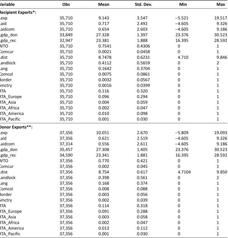
(5) Table 1. Summary statistics. Variable. Obs. Mean. Std. Dev.. Min. Max. Recipient Exports*: Lexp Laid Laidcom Lgdp_don Lgdp_rec WTO Comcur Ldist Landlock Lang Comcol Border Smctry RTA RTA_Europe RTA_Asia RTA_Africa RTA_America RTA_Pacific. 35,710 35,710 35,710 33,849 32,947 35,710 35,710 35,710 35,710 35,710 35,710 35,710 35,710 35,710 35,710 35,710 35,710 35,710 35,710. 9.143 0.717 0.654 27.328 23.381 0.7541 0.0021 8.7478 0.4112 0.1642 0.0075 0.0032 0.0016 0.116 0.096 0.004 0.002 0.010 0.001. 3.547 2.492 2.603 1.397 1.888 0.4306 0.0458 0.6231 0.5659 0.3704 0.0861 0.0567 0.0399 0.320 0.294 0.059 0.047 0.098 0.030. −5.521 −4.605 −4.605 23.376 16.395 0 0 4.710 0 0 0 0 0 0 0 0 0 0 0. 19.517 9.326 9.186 30.523 28.592 1 1 9.846 2 1 1 1 1 1 1 1 1 1 1. Donor Exports**: Lexp Laid Laidcom Lgdp_don Lgdp_rec WTO Comcur Ldist Landlock Lang Comcol Border Smctry RTA RTA_Europe RTA_Asia RTA_Africa RTA_America RTA_Pacific. 37,356 37,356 37,314 35,457 34,590 37,356 37,356 37,356 37,356 37,356 37,356 37,356 37,356 37,356 37,356 37,356 37,356 37,356 37,356. 10.051 0.621 0.556 27.308 23.341 0.770 0.002 8.754 0.398 0.168 0.008 0.003 0.002 0.114 0.091 0.003 0.002 0.013 0.001. 2.670 2.519 2.611 1.405 1.881 0.421 0.045 0.617 0.561 0.374 0.088 0.056 0.039 0.318 0.288 0.058 0.047 0.112 0.030. −5.809 −4.605 −4.605 23.376 16.395 0 0 4.7104 0 0 0 0 0 0 0 0 0 0 0. 19.093 9.326 9.186 30.523 28.592 1 1 9.850 2 1 1 1 1 1 1 1 1 1 1. Notes: * Dataset used in Tables 2 and A.5 and first part of Tables A.7 and A.8. ** Dataset used in Tables 3 and A.6 and second part of Tables A.7 and A.8. L denotes natural logs.. where aid denotes net bilateral official development aid (disbursements). The Z1 variables are the natural logs of GDPs for the donor and recipient countries as well as the standard gravity variables; namely, distance between trading countries and dummy variables for common language, past or current colonial relationship and RTA (we omit subscripts for simplicity). In the preferred panel data specification, the effect of the bilateral time-invariant gravity variables will be subsumed in the dyadic fixed effects and the effect of GDPs on the timevariant MRT.. Politics and Governance, 2019, Volume 7, Issue 2, Pages 29–52. First, consider the exogeneity assumption: E(Z′1 uijt ) = 0.. (2). The reduced form for laid is: laidijt = Z𝜋2 + 𝜀ijt ,. (3). where Z includes (in addition to the exogenous variables in Z1 ) aid commitments (aid commitments were lagged two periods to avoid endogeneity concerns), and country-specific fixed effects as exclusion variables.. 33.

(6) The linear projection of uijt on 𝜀ijt is: uijt = 𝜌2 𝜀ijt + eijt .. for each recipient and time period: resxjt = 􏾜 Exp(û ijt ).. (4). Now plugging (4) into (1), we obtain: lxijt = Z1 𝛿1 + 𝛼1 laidijt + 𝜌2 𝜀ijt + eijt .. (6). i. (5). resaidjt = 􏾜 Exp(𝜀̂ijt ).. (7). i. The two-step procedure consists of first regressing bilateral aid on all the exogenous variables to obtain the reduced form residuals 𝜀̂ijt , and then regressing exports on a subset of the exogenous variables, bilateral aid and 𝜀̂ijt . We use the same two-step procedure for recipient exports and for donor exports (recipient imports). The OLS estimate from the second step in (5) is a control function estimate and gives consistent estimates. A simple test for the null of exogeneity is a t-statistic on the statistical significance of 𝜀̂ijt . We combine this control function approach with the use of panel data and three sets of fixed effects. These are bilateral fixed effects that control for the unobservable heterogeneity attached to each trade flow (ij) and donor-and-time (it) and recipient-and-time (jt) fixed effects as controls for MRT, which have to be considered when estimating theoretically-based gravity models using panel data. We use a first-step reduced form regression with aid as the response variable (based on Equation 3). The reduced form is a bilateral aid equation estimated with country fixed effects. For aid flows, the donor dummies reflect, in part, the effect of common aid policies that govern the way in which aid is distributed, while the recipient dummies are proxies for the political and institutional environment in the recipient countries. Reduced form estimations are presented separately for donor and recipient exports. Since we are also interested in the effect of trade policies in combination with aid policies, we add a number of RTA dummies and the interaction between RTA variables and aid to the empirical specification (based on equation 5). For instance, we show estimates for RTA agreements signed between recipient countries (developing countries) and donors in the following regions: Asia, America (North and South America), Africa, Europe and Pacific. The inclusion of interaction terms between the RTA dummies and development aid will allow us to investigate the extent to which trade and aid policies are complementary. The related literature has recognized the importance of evaluating the effects of foreign aid on the trade and economic growth of the recipient countries (Doucouliagos & Paldam, 2006, 2015). One of the main issues in such an analysis is the endogeneity of aid in the trade and growth equations. We tackle this issue as follows: First, we use the results from the estimations of bilateral exports (1) from recipient to donor countries (donor to recipient countries, see Frankel and Romer, 1999) and bilateral aid (3) to obtain the corresponding residuals. Then, we take the exponential of the residuals and aggregate them over all donors to obtain an estimate. Politics and Governance, 2019, Volume 7, Issue 2, Pages 29–52. Finally, these residuals in natural logs are used in a second-step estimation in which the dependent variables are the natural logs of total recipient exports, lxrec, and the natural log of recipient GDP per capita, lgdppc. The corresponding specifications are given by equations (7) and (8): lxrecjt = 𝛿j + 𝛼1 laidjt + 𝛼2 lgdppcjt + 𝛼3 CPIjt + 𝛼4 lxdonjt + 𝜌1 lresaidjt + 𝜌2 lresxdjt. (8). + 𝜃t + ejt . lgdppcjt = 𝛿j + 𝛼1 laidjt + 𝛼2 lpopjt + 𝛼3 lxrecht + 𝛼4 lxdonjt + 𝜌1 lresaidjt + 𝜌2 lresxdjt. (9). + 𝜌3 lresxrjt + 𝜃j + ejt . where l denotes natural logs, aid is bilateral aid, CPI denotes the consumer price index, xdon denotes donors’ exports and xrec recipients’ exports, 𝜃t denotes time fixed effects and 𝛿j denote country fixed effects. Lresxr and lresxd refer to the log of the aggregated exponential residuals from the corresponding gravity models for recipients’ exports and donors’ exports according to (6). The models are also estimated with IV using the second and third lag of aid commitments as instruments. Moreover, dynamic models that include the lagged dependent variables are also estimated as a robustness check. 4. Main Results A gravity model of trade with bilateral fixed effects and MRT is used to estimate the effects of bilateral aid on donor exports and recipient exports. The bilateral fixed effects control for unobservable country-pair heterogeneity as a source of the endogeneity of the aid variable, and the MRT allow us to estimate a theoretically-based structural gravity model, as described in the previous section. The results using this approach are shown in Table 2 for recipient exports and in Table 3 for donor exports. Regarding the target variable, bilateral aid, results indicates that it has a positive but small significant effect on recipient exports to donors (Table 2) and on donor exports to recipients (Table 3). This is also the case when aid is taken as endogenous in columns (4)–(6). The point estimate is 0.022 (Table 2, column 4) for recipient exports and 0.026 (Table 3, column 4) for donor exports, indicating that the effect is stronger for the latter. The estimates for donor exports are similar to those obtained in NowakLehmann et al. (2013) for the period 1988 to 2007 using Dynamic FGLS without MRT, but with leads and lags of the variables in first differences. Similar estimates were. 34.

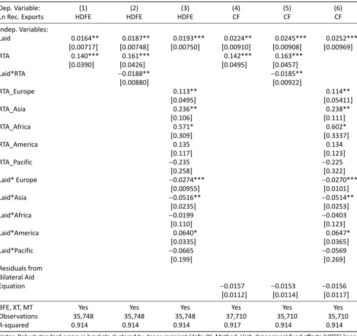
(7) Table 2. Gravity results for recipient exports. Dep. Variable: Ln Rec. Exports Indep. Variables: Laid RTA. (1) HDFE. (2) HDFE. 0.0164** [0.00717] 0.140*** [0.0390]. 0.0187** [0.00748] 0.161*** [0.0426] −0.0188** [0.00880]. Laid*RTA RTA_Europe. (3) HDFE 0.0193*** [0.00750]. (5) CF. 0.0224** [0.00910] 0.142*** [0.0495]. 0.0245*** [0.00908] 0.163*** [0.0457] −0.0185** [0.00922]. 0.113** [0.0495] 0.236** [0.106] 0.571* [0.309] 0.135 [0.117] −0.235 [0.258] −0.0274*** [0.00955] −0.0516** [0.0235] −0.0199 [0.110] 0.0640* [0.0335] −0.0665 [0.199]. RTA_Asia RTA_Africa RTA_America RTA_Pacific Laid* Europe Laid*Asia Laid*Africa Laid*America Laid*Pacific Residuals from Bilateral Aid Equation BFE, XT, MT Observations R-squared. (4) CF. Yes 35,748 0.914. Yes 35,748 0.914. Yes 35,748 0.914. (6) CF 0.0252*** [0.00969]. 0.114** [0.05411] 0.238** [0.111] 0.602* [0.3337] 0.134 [0.123] −0.225 [0.322] −0.0270*** [0.0101] −0.0514** [0.0253] −0.0403 [0.123] 0.0647* [0.0365] −0.0569 [0.269]. −0.0157 [0.0112]. −0.0153 [0.0114]. −0.0156 [0.0117]. Yes 37,710 0.917. Yes 35,710 0.914. Yes 35,710 0.914. Notes: Robust standard errors in brackets clustered by donor-recipient (default). Method: High-dimensional fixed effects (HDFE) linear regression. Fixed effects include: donor-year (XT), recipient-year (MT), donor-recipient (BFE). *** p < 0.01, ** p < 0.05, * p < 0.1. CF denotes Control Function Approach. All models estimated with the Stata command reghdfe from Correia (2017). Bootstrapped standard errors in columns 3–6 (1000 replications).. also obtained for donor exports using GMM in a dynamic setting (as shown in Martínez-Zarzoso et al., 2014). In contrast to Nowak-Lehmann et al. (2013), we also obtain statistically significant coefficients for recipient exports. However, only the results concerning donor exports are robust when a PPML (Poisson pseudo-maximum likelihood) estimator—a technique that tackles several econometric issues, including zero flows, selection bias and heteroskedasticity—is used (see the results in Tables A.5 and A.6). In the case of recipient exports, bilateral aid turns out to be non-statistically significant when PPML is used (Table A.5), in line with previous literature. 3. We add to the model the average effect of RTAs and its interaction with bilateral aid in column (2) and the effects of specific trade agreements and their interactions with bilateral aid in column (3) of Tables 2 and 3. The results show that the interaction between the RTA variable and bilateral aid is negative and statistically significant, indicating that the positive effect found for the aid variable vanishes for countries that have common RTAs. In particular, the partial effect of aid on recipient exports when RTA = 1, calculated using the results in column (2) of Tables (2) and (3)3 , is not statistically significant. Therefore aid is only statistically significant on average when. The marginal effect of aid on trade has been calculated using a test of joint statistical significance (lincom in Stata).. Politics and Governance, 2019, Volume 7, Issue 2, Pages 29–52. 35.

(8) Table 3. Gravity results for donor exports. Dep. Variable: Ln donor exports Indep. Variables: Laid RTA. (1) HDFE 0.0297*** [0.00396] 0.173*** [0.0242]. Laid*RTA. (2) HDFE 0.0338*** [0.00413] 0.204*** [0.0257] −0.0329*** [0.00493]. RTA_Europe. (3) HDFE 0.0344*** [0.00414]. 0.0259*** [0.00488] 0.176*** [0.0242]. (5) CF 0.0296*** [0.00499] 0.207*** [0.0258] −0.0335*** [0.00494]. 0.218*** [0.0307] 0.0801 [0.0797] 0.244 [0.183] 0.121*** [0.0453] −0.903*** [0.242] −0.0409*** [0.00551] 0.0271 [0.0190] 0.0307 [0.0825] −0.0276** [0.0118] −0.695*** [0.188]. RTA_Asia RTA_Africa RTA_America RTA_Pacific Laid*Europe Laid*Asia Laid*Africa Laid*America Laid*Pacific Residuals from Bilateral Aid Equation Observations R-squared. (4) CF. 37,356 0.952. 37,356 0.952. 37,356 0.952. (6) CF 0.0302*** [0.00501]. 0.222*** [0.0307] 0.0803 [0.0797] 0.248 [0.186] 0.121*** [0.0453] −0.905*** [0.241] −0.0414*** [0.00551] 0.0272 [0.0190] 0.0276 [0.0844] −0.0283** [0.0118] −0.699*** [0.188]. 0.0101* [0.00610]. 0.0110* [0.00610]. 0.0111* [0.00610]. 37,314 0.952. 37,314 0.952. 37,314 0.952. Notes: Robust standard errors in brackets clustered by donor-recipient (default). Method: High-dimensional fixed effects (HDFE) linear regression. Fixed effects include: donor-year, recipient-year, donor-recipient. *** p < 0.01, ** p < 0.05, * p < 0.1. CF denotes Control Function Approach. All models estimated with the Stata command reghdfe from Correia (2017). Bootstrapped standard errors in columns 3–6 (1000 replications).. there are no RTAs between the donor and the recipient country. The estimated coefficient for pairs of countries without RTAs indicates that a 10 percent increase in bilateral aid raises recipient exports by about 0.24 percent (column 5, Table 2), whereas for donor exports the corresponding effect is around 0.3 percent (column 5, Table 3). Moreover, the coefficient estimated for the RTA variable indicates that RTAs increase exports by around 17 percent4 for recipients and by 22 percent for donors for country pairs without aid link. These effects decrease with the amount of aid given, as indicated by the negative effect of the interaction variable (Laid * RTA). Results in column (3) of both tables show that the effect is heterogeneous and varies by agreement. For in4. stance, the bilateral RTAs signed mostly between the EU and EFTA (Europe) and recipient countries have a positive and significant effect on recipient exports—and also on donor exports—but this effect decreases with the amount of aid given. This is also the case for RTAs in Asia (see Table A.4 for a list of agreements included). In terms of the RTAs signed by American countries, they seem to exert a statistically significant effect on donor exports only, and this effect also decreases with the amount of aid given. For the agreement involving the Pacific region (Australia–Singapore and TPP: Trans-Pacific Partnership Agreement), no significant effect of the RTAs on recipient exports is found, whereas the effect is negative and significant for donor exports.. The effect is calculated as Exp(0.163 − 1)*100 using the coefficient of the RTA variable in column (5) of Table 2.. Politics and Governance, 2019, Volume 7, Issue 2, Pages 29–52. 36.

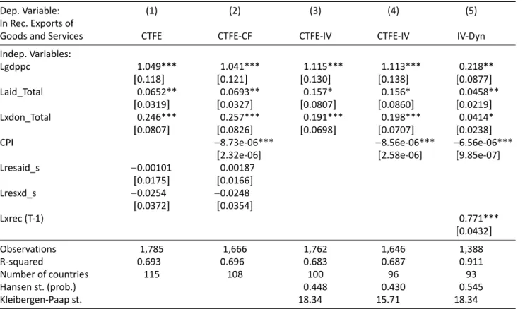
(9) Next, we estimate the effect of aid on aggregate recipient exports and on income per capita in the recipient countries by using the control function approach and alternative IV methods. The main results are presented in Tables 4 (for exports) and 5 (for income). Column (1) shows the FE results and column (2) the results of the control function approach, when the aggregated residuals from the first step estimations of bilateral aid and bilateral exports are added as regressors. In columns (3)–(4), the models are estimated using IV for aid, while column (5) presents the results of a dynamic model that uses IV for aid and for the lagged dependent variable. The results in Table 4 indicate that greater amounts of aid received and more imports from all donors lead to an increase in recipient exports, given that significant and positive effects are shown for foreign aid and for donors’ exports. In particular, a 10 percent increase in ODA raises recipient exports by around 0.6 percent when using the control function approach, and the point estimate increases to 1.6 when using IV; however, the effect is statistically significant only at the 10 percent level. In addition, for each 10 percent increase in donor exports, recipient exports increase by around 2.6 percent (column 2, Table 4). These results are robust to the addition of control variables (column 4) and the lagged dependent variable (column 5) to the model. The long-run effects in. column (5) can be calculated by dividing the point coefficients by (1–0.77), with 0.77 being the coefficient of the lagged dependent variable. Tests for the validity of the instruments are included in the last two rows of Table 4. The Hansen test indicates that we cannot reject the validity of the instruments and the Kleibergen-Paap statistic indicates that the instruments are not weak. Column (1) in Table 5 shows the effect of trade on the recipient’s income per capita. A one percent increase in exports from recipients to donors raises the income per capita in the recipient country by around 0.12 percent. Moreover, the same increase in donors’ exports increases that income level by around 0.2 percent. As in other studies (Nowak-Lehmann et al., 2013), the aid coefficient is not statistically significant in Table 5. However, aid is found to exert an indirect effect on income through trade, given that aggregate aid and imports from the donors are associated with higher recipient exports (Table 4), and higher recipient exports have a positive effect on income (Table 5). The estimated coefficients in columns (1) and (2) of Table 5 are robust to changes in the specification and to the addition to a number of control variables. In particular, column (3) presents the results when population, foreign direct investment, remittances, and gross capital formation are added to the model; the main difference is the reduction in the coeffi-. Table 4. Regression results for aggregate recipient exports. Dep. Variable: ln Rec. Exports of Goods and Services Indep. Variables: Lgdppc Laid_Total Lxdon_Total. (1). (2). (3). (4). (5). CTFE. CTFE-CF. CTFE-IV. CTFE-IV. IV-Dyn. 1.115*** [0.130] 0.157* [0.0807] 0.191*** [0.0698]. 1.113*** [0.138] 0.156* [0.0860] 0.198*** [0.0707] −8.56e-06*** [2.58e-06]. 1.049*** [0.118] 0.0652** [0.0319] 0.246*** [0.0807]. CPI Lresaid_s Lresxd_s. −0.00101 [0.0175] −0.0254 [0.0372]. 1.041*** [0.121] 0.0693** [0.0327] 0.257*** [0.0826] −8.73e-06*** [2.32e-06] 0.00187 [0.0166] −0.0248 [0.0354]. Lxrec (T-1) Observations R-squared Number of countries Hansen st. (prob.) Kleibergen-Paap st.. 0.218** [0.0877] 0.0458** [0.0219] 0.0414* [0.0238] −6.56e-06*** [9.85e-07]. 0.771*** [0.0432] 1,785 0.693 115. 1,666 0.696 108. 1,762 0.683 100 0.448 18.34. 1,646 0.687 96 0.430 15.71. 1,388 0.911 93 0.545 18.34. Notes: Robust standard errors in brackets. *** p < 0.01, ** p < 0.05, * p < 0.1. CFE denotes country fixed effects, CTFE denotes country and time fixed effects, CF Control Function Approach and IV instrumental variables. The definition of the variables can be found in Table A2 and lresaid_s and lresxd_s are obtained from the estimated residuals of the aid and the donors’ exports models, respectively. Hansen st. (prob.) is the probability associated to the Hansen test, which indicate that we cannot reject the validity of the instruments. Kleibergen-Paap statistic is a test for weak instruments, which result indicates that the instruments are not weak.. Politics and Governance, 2019, Volume 7, Issue 2, Pages 29–52. 37.

(10) Table 5. Regression results for recipient income per capita. Dep. Variable: lgdppc Indep. Variables: Laid_Total Lxrec_Total Lxdon_Total. (1) CTFE. (2) CTFE-CF. (3) CTFE_CF. −0.0165 [0.0144] 0.121*** [0.0291] 0.208*** [0.0422]. −0.0145 [0.0156] 0.119*** [0.0289] 0.207*** [0.0424]. −0.00436 [0.0106] 0.0939*** [0.0331] 0.0855*** [0.0286] −0.911*** [0.129] 0.00168 [0.00469] 0.00183 [0.00876] 0.110*** [0.0283] 0.00879 [0.00599] 0.000895 [0.00662] −0.0239 [0.0144]. Lpop Lfdi Lrem Lgcf Lresaid_s. 0.00485 [0.0105] −0.0135 [0.0106] −0.0452** [0.0196]. Lresxr_s Lresxd_s. (4) CTFE-IV 0.00130 [0.0323] 0.121*** [0.0301] 0.223*** [0.0362]. (5) CTFE-IV. (6) IV-Dyn. 0.0261 [0.0218] 0.108*** [0.0333] 0.0782*** [0.0288] −0.960*** [0.142] 0.00210 [0.00449] 0.00223 [0.00872] 0.120*** [0.0274]. 0.00646 [0.00694] 0.0285*** [0.00491] 0.0176* [0.0106] −0.245*** [0.0293]. Lgdppc(T-1) Observations R-squared Number of countries Hansen st. (prob.) Kleibergen-Paap st.. 0.0372*** [0.00811]. 0.799*** [0.0168] 2,248 0.667 126. 2,241 0.670 121. 1,447 0.843 100. 2,235 0.663 122 0.283 19.39. 1,438 0.836 96 0.0239 12.54. 1,697 0.961 110 0.793 20.59. Notes: Robust standard errors in brackets. *** p < 0.01, ** p < 0.05, * p < 0.1. CFE denotes country fixed effects, CTFE denotes country and time fixed effects, CF Control Function Approach and IV instrumental variables. The definition of the variables can be found in Table A2. lresaid_s, lresxr_s and lresxd_s are obtained from the estimated residuals of the aid, the recipients’ exports and the donors’ exports models, respectively. Hansen st. (prob.) is the probability associated to the Hansen test, which indicate that we cannot reject the validity of the instruments. Kleibergen-Paap statistic is a test for weak instruments, which result indicates that the instruments are not weak.. cient of donor exports, which is in part due to the smaller sample of countries for which data are available (121 in column 2 compared to 100 in column 3). In columns (4) and (5), the aid variable is instrumented with the first and second lag of aggregate aid commitments and the results remain similar to those in columns (2) and (3) using the control function approach. Finally, in column (5), the lagged dependent variable of income per capita is added to the model to incorporate dynamics. The coefficient of the lagged income variable is positive and significant, as expected, and the results for recipient exports and donor exports remain positive and significant: the long-run effects are 0.14 and 0.08 for each one percent increase in recipient and donor exports, respectively. As in Table 4, the last two rows of Table 5 include tests for the validity of the instruments and for weak instruments. The control function approach allows us to test for the endogeneity of aid and trade variables in the recipient exports and income equations estimated in Tables 4 and 5.. The corresponding t-tests on the residuals from the firststep equations (for exports and for development aid) indicate that the coefficients of the residuals are generally not statistically significant when the model is estimated with country and time fixed effects, suggesting that the use of panel data mitigates potential endogeneity.. Politics and Governance, 2019, Volume 7, Issue 2, Pages 29–52. 38. 5. Robustness Checks As a first robustness check, we have estimated the gravity models for recipient exports and imports using the usual gravity controls; namely, income in the trading countries and dummy variables for common language, common border, colonial relationship and belonging to the same country in the past. The results are shown in Table A.7. In general, the aid coefficient is positive and significant, and higher in magnitude than in the main results. This is as expected since the models in Table A.7 do not control for time-variant MRT, nor for all the bilateral unobserved.

(11) heterogeneity in the gravity model. We have also run separate models for different regions. Using the World Bank classification, we divide the world into regions as indicated in Table A.8. The results for recipient exports shown in column (1) indicate that it is mainly aid sent to the Latin American and Caribbean region and to South Asian countries that has been effective in increasing recipient exports. Concerning donor exports, the results are shown in column (2) and indicate that aid to East Asia & Pacific, to Europe & Central Asia, to South Asia, and to Sub-Saharan Africa increase exports, whereas the aid coefficient for Latin America & Caribbean and Middle East & North Africa is not statistically significant. The income per capita model was also estimated in first differences with IV to avoid potential issues with spurious correlations, and the results hold (see Table A.9). Finally, the model was also estimated for several lags of the aggregate aid variable and the results indicate that the aid was statistically significant in the income model when using the fifth lag as regressor and the sixth-to-tenth lags as instruments. This is in line with recent reviews of the aid-growth literature (Table A.10).. also grateful to the financial support received from Project ECO2017-83255-C3-3-P (AEI, FEDER, EU) and from project UJI-B2017-33. Conflict of Interests The author declares no conflict of interests. References. I would like to thank the anonymous referees and the editors for their helpful comments and suggestions. I am. Addison, T., Morrisey, O., & Tarp, F. (2017). The macroeconomics of aid: Overview. Journal of Development Studies, 53(7), 987–997. Alcalá, F., & Ciccone, A. (2004). Trade and productivity. The Quarterly Journal of Economics, 119(2), 621–645. Anderson, J. E. (1979). A theoretical foundation for the gravity equation. American Economic Review, 69(1), 106–116. Anderson, J. E., & Van Wincoop, E. (2003). Gravity with gravitas: A solution to the border puzzle. American Economic Review, 93, 170–192. Arndt, C., Jones, S., & Tarp, F. (2010). Aid, growth, and development: Have we come full circle? Journal of Globalization and Development, 1(2), 27. Arndt, C., Jones, S., & Tarp, F. (2015). Assessing foreign aid’s long run contribution to growth and development. World Development, 69, 6–18. Arndt, C., Jones, S., & Tarp, F. (2016). What is the aggregate economic rate of return to foreign aid? World Bank Economic Review, 30, 446–474. Arvin, M., & Baum, C. (1997). Tied and untied foreign aid: Theoretical and empirical analysis. Keio Economic Studies, 34(2), 71–79. Arvin, M., & Choudhry, S. (1997). Untied aid and exports: Do untied disbursements create goodwill for donor exports? Canadian Journal of Development Studies, 18(1), 9–22. Baier, S. L., & Bergstrand, J. H. (2009). Bonus vetus OLS: A simple method for approximating international trade-cost effects using the gravity equation. Journal of International Economics, 77(1), 77–85. Bergstrand, J. H. (1985). The gravity equation in international trade: Some microeconomic foundations and empirical evidence. The Review of Economics and Statistics, 67, 474–481. Bergstrand, J. H. (1989). The generalized gravity equation, monopolistic competition, and the factorproportions theory in international trade. Review of Economics and Statistics, 71(1), 143–153. Burnside, C., & Dollar, D. (2000). Aid, policies, and growth. American Economic Review, 90, 847–868. Cadot, O., Fernandes, A., Gourdon, J., Matto, A., & de Melo, J. (2014). Evaluating aid for trade. A survey of recent studies. The World Economy, 37(4), 516–529. Chenery, H. B., & Strout, A. M. (1966). Foreign assistance and economic development. American Economic Review, 56(4), 679–733. Collier, P., & Dollar, D. (2001). Can the world cut poverty. Politics and Governance, 2019, Volume 7, Issue 2, Pages 29–52. 39. 6. Conclusion This article reviews the recent literature on the bilateral trade and aid link that uses the gravity model as the main analytical framework. Existing studies find a robust positive effect of bilateral aid on bilateral exports from donor to recipient countries. The findings also indicate that there is a small but non-robust effect of bilateral aid on recipient exports. The claim for causality running from aid to exports is supported by use of methods that account for the endogeneity of aid in the bilateral trade equation. This article confirms the abovementioned findings and adds trade policy variables, specifically RTA dummy variables, to the main setting. It has been argued that in some cases, donors will seek to combine closer trade relations with more aid, whereas in other cases, aid and trade regional policies are unrelated. The results of this article support the view that donors give aid to countries with which they have weak trade links with the aim of establishing closer relations. Finally, when studying the effect of total aid on total recipient exports and GDP per capita, we find that the effect of aid on recipient exports is statistically significant and that aggregate exports and imports seems to have a positive and significant effect on the GDP per capita of the recipient countries. Hence, the part of trade that has been incentivized by foreign aid appears to foster economic development. Acknowledgments.

(12) in half? How policy reform and effective aid can meet international development goals. World Development, 29(11), 1787–1802. Correia, S. (2017). Linear models with high-dimensional fixed effects: An efficient and feasible estimator (Working Paper). Retrieved from http://scorreia. com/research/hdfe.pdf Crivelli, E., & Gupta, S. (2017). Does conditionality mitigate the potential negative effect of aid on revenues? Journal of Development Studies, 53, 1057–1074. Dalgaard, C. J., & Hansen, H. (2000). On aid, growth and good policies. Journal of Development Studies, 37(6), 17–41. Dalgaard, C. J., Hansen, H., & Tarp, F. (2004). On the empirics of foreign aid and growth. Economic Journal, 114(496), F191–F216. De Sousa, J. (2012). The currency union effect on trade is decreasing over time. Economics Letters, 117(3), 917–920. Dollar, D., & Kraay, A. (2003). Institutions, trade and growth. Journal of Monetary Economics, 50, 133–162. Doucouliagos, H., & Paldam, M. (2006). Aid effectiveness on accumulation. A meta study. Kyklos, 59, 227–254. Doucouliagos, H., & Paldam, M. (2008). Aid effectiveness on growth: A meta study. The European Journal of Political Economy, 24(1), 1–24. Doucouliagos, H., & Paldam, M. (2015). Finally a breakthrough? The recent rise in the size of the estimates of aid effectiveness. In M. Arvin & B. Lew. (Eds), Handbook on the economics of foreign aid (pp. 325–347). Trent: Edward Elgar Publishing. Edwards, S. (2005). Economic development and the effectiveness of foreign aid: A historical perspective. Kyklos, 68(3), 277–316. Frankel, J. A., & Romer, D. H. (1999). Does trade cause growth? American Economic Review, 89(3), 379–399. Griffin, K. B., & Enos, J. L. (1970). Foreign assistance: Objectives and consequences. Economic Development and Cultural Change, 18, 313–327. Hansen, H., & Rand, J. (2014). Danish exports and Danish bilateral aid. Evaluation study. Copenhagen: Ministry of Foreign Affair of Denmark, Danida. Hansen, H., & Tarp, F. (2000). Aid effectiveness disputed. Journal of International Development, 12, 375–398. Hansen, H., & Tarp, F. (2001). Aid and growth regressions. Journal of Development Economics, 64, 547–570. Head, K., & Mayer, T. (2014). Gravity equations: Workhorse, toolkit, and cookbook. In G. Gopinath, E. Helpman, & K. Rogoff (Eds.), Handbook of international economics (Vol. 4, pp. 131–195). Amsterdam: Elsevier. Jepma, C. (1991). The tying of aid. Paris: OECD. Liu, A., & Tang, B. (2018). US and China aid to Africa: Impact on the donor-recipient trade relations. China Economic Review, 48, 46–65. Martínez-Zarzoso, I., Nowak-Lehmann, F., & Johannsen, F. (2012). Foreign aid, exports and development in. Euromed. Middle East Development Journal, 4(2), 1–24. Martínez-Zarzoso, I., Nowak-Lehmann, F., & Klasen, S. (2014). Does aid promote donor exports? Commercial interest versus instrumental philanthropy. Kyklos, 66, 559–587. Martínez-Zarzoso, I., Nowak-Lehmann, F., & Klasen, S. (2017). Aid and its impact on the donor’s export industry: The Dutch case. European Journal of Development Research, 29(4), 769–786. Martínez-Zarzoso, I., Nowak-Lehmann, F., Klasen, S., & Johannsen, F. (2016). Does German development aid promote German exports and German employment? Journal of Economics and Statistics, 236(1), 71–94. Martínez-Zarzoso, I., Nowak-Lehmann, F., Klasen, S., & Larch, M. (2009). Does German development aid promote German exports. German Economic Review, 10(3), 317–338. Martínez-Zarzoso, I., Nowak-Lehmann, F., & Rehwald, K. (2017). Is aid for trade effective? A panel quantile regression approach. Review of Development Economics, 21(4), e175–e203. McGillivray, M., Feeny, S., Hermes, N., & Lensink, R. (2006). Controversies over the impact of development aid: It works; it doesn’t; it can, but that depends… Journal of International Development, 18, 1031–1050. Morrisey, O. (2001). Does aid increase growth? Progress in Development Studies, 1(1), 37–50. Morrisey, O. (2005). Aid and government fiscal behaviour: Assessing recent evidence. World Development, 69, 98–105. Morrisey, O. (2006). Aid or trade, or aid and trade? Australian Economic Review, 39(1), 78–88. Nilsson, L. (1997). Aid and donor exports: The case of the EU Countries. In Essays on North–South trade (Lund Economic Studies, No. 70, pp. 47–77). Lund: Lund University. Nowak-Lehmann, F., Martínez-Zarzoso, I., Herzer, D., Klasen, S., & Cardozo, A. (2013). Does foreign aid promote recipient exports to donor countries? Review of World Economics, 149(3), 505–535. Nowak-Lehmann, F., Martínez-Zarzoso, I., Klasen, S., & Herzer, D. (2009). Aid and trade: A donor’s perspective. Journal of Development Studies, 45(7), 1184–1202. Otor, S. A. (2017). Japan’s official development assistance and exports to Asian countries: The donor’s perspective. Institutions and Economies, 6(3), 60–91. Pettersson, J., & Johansson, L. (2013). Aid, aid for trade, and bilateral trade: An empirical study. Journal of International Trade and Economic Development, 22(6), 866–894. Rajan, R., & Subramanian, A. (2008). Aid and growth: What does the cross-country evidence really show? The Review of Economics and Statistics, 90(4), 643–665. Silva, S. J., & Nelson, D. (2012). Does aid cause trade? Evi-. Politics and Governance, 2019, Volume 7, Issue 2, Pages 29–52. 40.

(13) dence from an asymmetric gravity model. The World Economy, 35(5), 545–577. Singh, T. (2010). Does international trade cause economic growth? A survey. The World Economy, 33, 1517–1564. Temple, J., & Van de Sijpe, N. (2017). Foreign aid and domestic absorption. Journal of International Economics, 108, 431–443. The World Bank. (2018). World Development Indicators. The World Bank. Washington, D.C.: The World Bank. Retrieved from http://data.worldbank.org/ data-catalog/world-development-indicators Tinbergen, J. (1962). An analysis of world trade flows. In J. Tinbergen (Ed.), Shaping the world economy. New York, NY: Twentieth Century Fund. Vijil, M. (2014). Aid for trade effectiveness: Complemen-. tarities with economic integration. The World Economy, 37(4), 555–566. Wagner, D. (2003). Aid and trade: An empirical study. Journal of the Japanese and International Economies, 17, 153–173. White, H. (1992). The macroeconomic impact of development aid: A critical survey. Journal of Development Studies, 28(2), 163–240. Wooldridge, J. M. (2010). Econometric analysis of cross section and panel data (2nd ed.). Cambridge, MA: MIT Press. Zarin-Nejadan, M., Monteiro, J. A., & Noormamode, S. (2008). The impact of official development assistance on donor country exports: Some empirical evidence for Switzerland. Neuchatel: Institute for Research in Economics, University of Neuchatel.. About the Author Inmaculada Martínez-Zarzoso is Apl. Professor of Economics and board member of the Global Center of Migration (CeMig) at the University of Göttingen in Germany. She is also Professor of Economics at the University Jaume I in Spain and board member of the International Network for Economic Research. She holds a PhD in economics from the University of Birmingham and has advised a number of international and national institutions, including The World Bank, the OECD, the Commonwealth Secretariat, the German Ministry of Development, the Netherlands Ministry of Foreign Affairs, and the Spanish Ministry of Transport and Infrastructure.. Politics and Governance, 2019, Volume 7, Issue 2, Pages 29–52. 41.

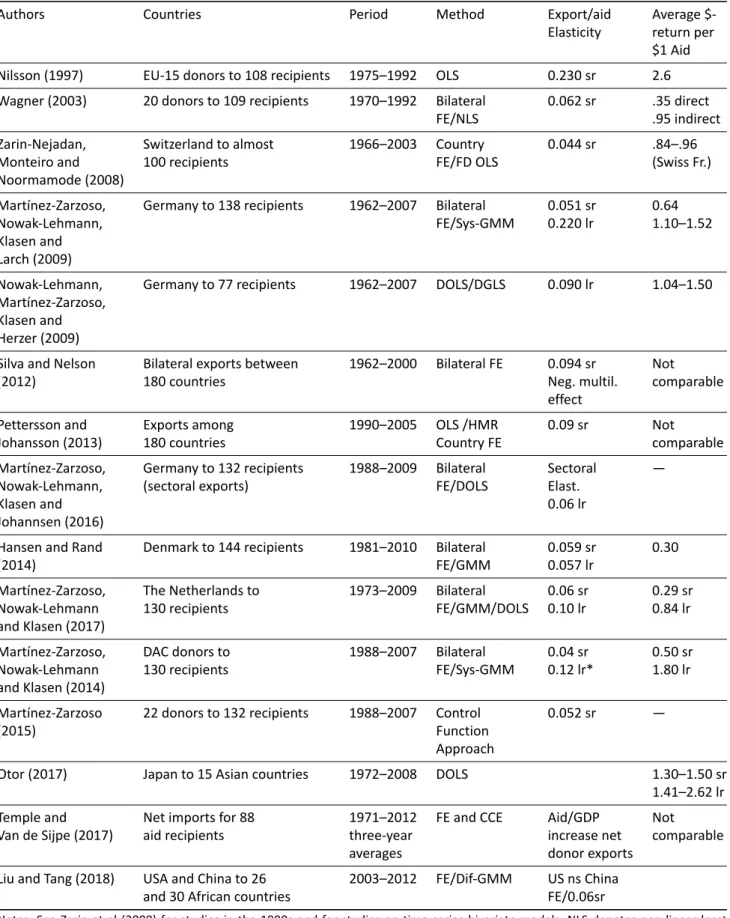
(14) Appendix Table A.1. Overview of studies on the effects of ODA on donor exports. Authors. Countries. Period. Method. Export/aid Elasticity. Average $return per $1 Aid. Nilsson (1997). EU-15 donors to 108 recipients. 1975–1992. OLS. 0.230 sr. 2.6. Wagner (2003). 20 donors to 109 recipients. 1970–1992. Bilateral FE/NLS. 0.062 sr. .35 direct .95 indirect. Zarin-Nejadan, Monteiro and Noormamode (2008). Switzerland to almost 100 recipients. 1966–2003. Country FE/FD OLS. 0.044 sr. .84–.96 (Swiss Fr.). Martínez-Zarzoso, Nowak-Lehmann, Klasen and Larch (2009). Germany to 138 recipients. 1962–2007. Bilateral FE/Sys-GMM. 0.051 sr 0.220 lr. 0.64 1.10–1.52. Nowak-Lehmann, Martínez-Zarzoso, Klasen and Herzer (2009). Germany to 77 recipients. 1962–2007. DOLS/DGLS. 0.090 lr. 1.04–1.50. Silva and Nelson (2012). Bilateral exports between 180 countries. 1962–2000. Bilateral FE. 0.094 sr Neg. multil. effect. Not comparable. Pettersson and Johansson (2013). Exports among 180 countries. 1990–2005. OLS /HMR Country FE. 0.09 sr. Not comparable. Martínez-Zarzoso, Nowak-Lehmann, Klasen and Johannsen (2016). Germany to 132 recipients (sectoral exports). 1988–2009. Bilateral FE/DOLS. Sectoral Elast. 0.06 lr. —. Hansen and Rand (2014). Denmark to 144 recipients. 1981–2010. Bilateral FE/GMM. 0.059 sr 0.057 lr. 0.30. Martínez-Zarzoso, Nowak-Lehmann and Klasen (2017). The Netherlands to 130 recipients. 1973–2009. Bilateral FE/GMM/DOLS. 0.06 sr 0.10 lr. 0.29 sr 0.84 lr. Martínez-Zarzoso, Nowak-Lehmann and Klasen (2014). DAC donors to 130 recipients. 1988–2007. Bilateral FE/Sys-GMM. 0.04 sr 0.12 lr*. 0.50 sr 1.80 lr. Martínez-Zarzoso (2015). 22 donors to 132 recipients. 1988–2007. Control Function Approach. 0.052 sr. —. Otor (2017). Japan to 15 Asian countries. 1972–2008. DOLS. Temple and Van de Sijpe (2017). Net imports for 88 aid recipients. 1971–2012 three-year averages. FE and CCE. Aid/GDP increase net donor exports. Liu and Tang (2018). USA and China to 26 and 30 African countries. 2003–2012. FE/Dif-GMM. US ns China FE/0.06sr. 1.30–1.50 sr 1.41–2.62 lr Not comparable. Notes: See Zarin et al (2008) for studies in the 1990s and for studies on time-series bivariate models. NLS denotes non-linear least squares. FE denotes fixed effects, Sys-GMM denotes System Generalized Method of Moments, DOLS/DGLS denotes dynamic OLS and dynamic generalized least squares. SR denotes short run (from a static model) and LR long run estimates (from a dynamic model). HMR denotes Helpman, Melitz and Rubinstein (2008). *Calculated as an average of the LR coefficients of three periods.. Politics and Governance, 2019, Volume 7, Issue 2, Pages 29–52. 42.

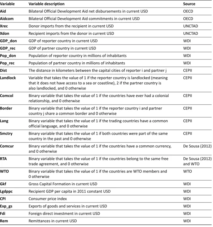
(15) Table A.2. List of variables, definitions and sources. Variable. Variable description. Source. Aid. Bilateral Official Development Aid net disbursements in current USD. OECD. Aidcom. Bilateral Official Development Aid commitments in current USD. OECD. Xrec. Donor imports from the recipient in current USD. UNCTAD. Xdon. Recipient imports from the donor in current USD. UNCTAD. GDP_don. GDP of reporter country in current USD. WDI. GDP_rec. GDP of partner country in current USD. WDI. Pop_don. Population of reporter country in millions of inhabitants. WDI. Pop_rec. Population of partner country in millions of inhabitants. WDI. Dist. The distance in kilometers between the capital cities of reporter i and partner j. CEPII. Landlock. Variable that takes the value of 1 if the reporter country is landlocked (meaning that it does not have access to a sea or coastline), 2 if the partner country is also landlocked, and 0 otherwise. CEPII. Comcol. Binary variable that takes the value of 1 if the countries have ever had a colonial relationship, and 0 otherwise. CEPII. Border. Binary variable that takes the value of 1 if the reporter country i and partner country j share a common border and 0 otherwise. CEPII. Lang. Binary variable that takes the value of 1 if the trading countries have a common official language, and 0 otherwise. CEPII. Smctry. Binary variable that takes the value of 1 if both countries were part of the same country in the past and 0 otherwise. CEPII. Comcur. Binary variable that takes the value of 1 if the countries have a common currency, and 0 otherwise. De Sousa (2012). RTA. Binary variable that takes the value of 1 if the countries belong to the same free trade agreement, and 0 otherwise. De Sousa (2012) and WTO. WTO. Binary variable that takes the value of 1 if the countries are WTO members and 0 otherwise. WTO. Gkf. Gross Capital Formation in current USD. WDI. Lgdppc. Recipient GDP per capita in 2011 constant USD. WDI. CPI. Consumer price index. WDI. Exp_gs. Exports of goods and services in current USD. WDI. Fdi. Foreign direct investment in current USD. WDI. Rem. Remittances in current USD. WDI. Politics and Governance, 2019, Volume 7, Issue 2, Pages 29–52. 43.

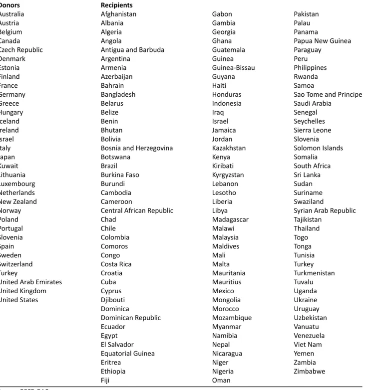
(16) Table A.3. List of countries. Donors Australia Austria Belgium Canada Czech Republic Denmark Estonia Finland France Germany Greece Hungary Iceland Ireland Israel Italy Japan Kuwait Lithuania Luxembourg Netherlands New Zealand Norway Poland Portugal Slovenia Spain Sweden Switzerland Turkey United Arab Emirates United Kingdom United States. Recipients Afghanistan Albania Algeria Angola Antigua and Barbuda Argentina Armenia Azerbaijan Bahrain Bangladesh Belarus Belize Benin Bhutan Bolivia Bosnia and Herzegovina Botswana Brazil Burkina Faso Burundi Cambodia Cameroon Central African Republic Chad Chile Colombia Comoros Congo Costa Rica Croatia Cuba Cyprus Djibouti Dominica Dominican Republic Ecuador Egypt El Salvador Equatorial Guinea Eritrea Ethiopia Fiji. Gabon Gambia Georgia Ghana Guatemala Guinea Guinea-Bissau Guyana Haiti Honduras Indonesia Iraq Israel Jamaica Jordan Kazakhstan Kenya Kiribati Kyrgyzstan Lebanon Lesotho Liberia Libya Madagascar Malawi Malaysia Maldives Mali Malta Mauritania Mauritius Mexico Mongolia Morocco Mozambique Myanmar Namibia Nepal Nicaragua Niger Nigeria Oman. Pakistan Palau Panama Papua New Guinea Paraguay Peru Philippines Rwanda Samoa Sao Tome and Principe Saudi Arabia Senegal Seychelles Sierra Leone Slovenia Solomon Islands Somalia South Africa Sri Lanka Sudan Suriname Swaziland Syrian Arab Republic Tajikistan Thailand Togo Tonga Tunisia Turkey Turkmenistan Tuvalu Uganda Ukraine Uruguay Uzbekistan Vanuatu Venezuela Viet Nam Yemen Zambia Zimbabwe. Source: OECD-DAC.. Politics and Governance, 2019, Volume 7, Issue 2, Pages 29–52. 44.

(17) Table A.4. List of free trade agreements. Europe EU-South Africa EU-Albania EU-Bosnia Turkey-Bosnia&Herz. EU-Slovenia EU-Chile EU-Cameroon EU-Colombia Croatia-Turkey EU-Algeria EFTA-Albania EFTA-Bosnia&Herz. EFTA-Chile EFTA-Colombia EFTA-Costa Rica EFTA-Colombia EFTA-Egypt EFTA-Israel EFTA-Jordan EFTA-Libya EFTA-Morocco EFTA-Mexico EFTA-Panama EFTA-Peru EFTA-Tunisia EFTA-Turkey EFTA-Ukraine EU-Egypt EU-East Africa EU-Canada EU-Fiji EU-Georgia EU-Jordan EU-Libya EU-Morocco EU-Mexico EU-Peru EU-Singapore EU-Syria EU-Tunisia EU-Turkey Turkey-Israel EU-Ukraine EU-CARIFORUM. Asia ASEAN-Australia-New Zealand ASEAN-Japan Japan-Indonesia Japan-Malaysia Japan-Peru Japan-Philippines Japan-Vietnam Malaysia-Australia Malaysia-New Zealand Thailand-Japan Thailand- Australia Thailand-New Zealand Africa Egypt-Turkey Morocco-Turley South Africa CU Syria-Turkey Tunisia-Turkey. America Canada-Chile Canada-Colombia Canada-Costa Rica Canada-Honduras Canada-Jordan Canada-Panama Canada-Peru Chile-Australia Chile-Japan Mexico-Chile Mexico-Japan US-Mex-Can US-Chile US-Colombia USA-Israel US-Jordan US-Morocco US-Oman US-Panama US-Peru USA-CAFTA-Dominican Republic Pacific Australia-Singapore Trans-Pacific EPA. Source: WTO.. Politics and Governance, 2019, Volume 7, Issue 2, Pages 29–52. 45.

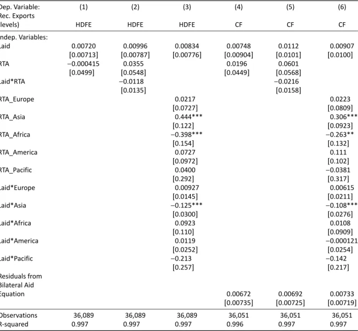
(18) Table A.5. PPML estimates for recipient exports. Dep. Variable: Rec. Exports (levels) Indep. Variables: Laid RTA. (1). (2). (3). (4). (5). (6). HDFE. HDFE. HDFE. CF. CF. CF. 0.00720 [0.00713] −0.000415 [0.0499]. 0.00996 [0.00787] 0.0355 [0.0548] −0.0118 [0.0135]. 0.00834 [0.00776]. 0.00748 [0.00904] 0.0196 [0.0449]. Laid*RTA RTA_Europe. 0.0217 [0.0727] 0.444*** [0.122] −0.398*** [0.154] 0.0727 [0.0972] 0.0400 [0.292] 0.00927 [0.0145] −0.125*** [0.0300] 0.0923 [0.110] 0.0119 [0.0252] −0.213 [0.257]. RTA_Asia RTA_Africa RTA_America RTA_Pacific Laid*Europe Laid*Asia Laid*Africa Laid*America Laid*Pacific Residuals from Bilateral Aid Equation Observations R-squared. 0.0112 [0.0101] 0.0601 [0.0568] −0.0216 [0.0158]. 36,089 0.997. 36,089 0.997. 36,089 0.997. 0.00907 [0.0100]. 0.0223 [0.0809] 0.306*** [0.0923] −0.263** [0.132] 0.111 [0.102] −0.0381 [0.317] 0.00615 [0.0211] −0.108*** [0.0276] 0.0108 [0.0909] −0.000121 [0.0254] −0.142 [0.217]. 0.00672 [0.00735]. 0.00692 [0.00725]. 0.00733 [0.00719]. 36,051 0.996. 36,051 0.997. 36,051 0.997. Notes: Standard errors in brackets. Method: PPML for structural gravity with high-dimensional fixed effects (HDFE). FE included: donoryear, recipient-year, donor-recipient. Clustered standard errors, clustered by donor-recipient (default). *** p < 0.01, ** p < 0.05. CF denotes Control Function Approach. The definition of the variables can be found in Table A2.. Politics and Governance, 2019, Volume 7, Issue 2, Pages 29–52. 46.

(19) Table A.6. PPML estimates for donor exports. Dep. Variable: Donor Exports (levels) Indep. Variables: Laid RTA. (1). (2). (3). (4). (5). (6). HDFE. HDFE. HDFE. CF. CF. CF. 0.00447 [0.00601] 0.181*** [0.0367]. 0.0182*** [0.00614] 0.253*** [0.0377] −0.0293*** [0.00843]. 0.00916** [0.00453] 0.171*** [0.0322]. Laid*RTA. 0.0187*** [0.00511] 0.250*** [0.0355] −0.0270*** [0.00721]. RTA_Europe. 0.0201*** [0.00500]. 0.168*** [0.0364] 0.447*** [0.115] −0.00941 [0.156] 0.429*** [0.0513] −0.391** [0.163] −0.0234*** [0.00693] −0.0681** [0.0266] −0.0974 [0.0830] −0.0455*** [0.0142] −0.334** [0.143]. RTA_Asia RTA_Africa RTA_America RTA_Pacific Laid*Europe Laid*Asia Laid*Africa Laid*America Laid*Pacific Residuals from Bilateral Aid Equation Observations R-squared. 37,879 0.999. 37,879 0.999. 37,879 0.999. 0.0211*** [0.00584]. 0.179*** [0.0377] 0.315*** [0.116] −0.0742 [0.151] 0.470*** [0.0551] −0.682*** [0.191] −0.0277*** [0.00857] −0.0425* [0.0248] −0.0658 [0.0606] −0.0598*** [0.0146] −0.412*** [0.115]. 0.00948* [0.00488]. 0.00949* [0.00498]. 37,837 0.998. 37,837 0.999. 0.00992** [0.00482] 37,837 0.999. Notes: Standard errors in brackets. Method: PPML for structural gravity with high-dimensional fixed effects (HDFE). FE included: donoryear, recipient-year, donor-recipient. Clustered standard errors, clustered by donor-recipient (default). *** p < 0.01, ** p < 0.05, * p < 0.1. CF denotes Control Function Approach. The definition of the variables can be found in Table A2.. Politics and Governance, 2019, Volume 7, Issue 2, Pages 29–52. 47.

(20) Table A.7. Gravity model with additional controls. Recipient exports Dep. Variable: Ln Exports Ind. Variables: Lgdp_rec Lgdp_don Laid RTA Laidrta WTO Comcur Ldist Landlock Lang Comcol Border Smctry Observations R-squared. Donor exports. (1) OLS-TFE. (2) OLS-TCFE. (3) OLS-TFE. (4) OLS-TCFE. 1.206*** [0.0329] 1.229*** [0.0231] 0.0330** [0.0161] 0.386*** [0.0886] 0.0268 [0.0294] 0.329*** [0.0990] 1.279** [0.604] −0.728*** [0.0585] −0.618*** [0.0764] 0.670*** [0.112] 1.009*** [0.266] 0.932** [0.443] 2.280*** [0.414]. 0.778*** [0.117] 0.685*** [0.0775] 0.106*** [0.0140] 0.240*** [0.0770] −0.0211 [0.0227] 0.206** [0.0838] −0.270 [0.474] −1.481*** [0.0803]. 0.822*** [0.0370] 0.0416 [0.0717] 0.159*** [0.00928] 0.183*** [0.0459] −0.0556*** [0.0139] 0.0966* [0.0529] 0.328 [0.554] −1.396*** [0.0515]. 0.479*** [0.102] −0.0278 [0.266] 0.255 [0.466] 1.094** [0.431]. 0.967*** [0.0157] 0.925*** [0.0218] 0.118*** [0.00967] 0.363*** [0.0535] −0.0104 [0.0172] 0.0875 [0.0541] 1.130 [1.057] −0.988*** [0.0378] −0.387*** [0.0469] 0.513*** [0.0711] 0.690*** [0.223] 0.533 [0.442] 0.906*** [0.325]. 33,253 0.628. 33,253 0.757. 35,052 0.767. 0.421*** [0.0665] 0.265 [0.206] 0.289 [0.581] 0.760* [0.443] 35,052 0.844. Notes: Robust standard errors in brackets. *** p < 0.01, ** p < 0.05, * p < 0.1. TFE denotes time fixed effects. TCFE denotes time and country fixed effects. The definition of the variables can be found in Table A2.. Politics and Governance, 2019, Volume 7, Issue 2, Pages 29–52. 48.

(21) Table A.8. Regional specific coefficients for aid. Dep. variable: Indep. Variables: Laid_EAP Laid_ECA Laid_LAC Laid_MENA Laid_SAS Laid_SSA RTA Laid*RTA Residuals from Bilateral Aid Equation Observations R-squared. (1) Ln Recipient Exports. (2) Ln Donor Exports. 0.0233 [0.0161] 0.0333 [0.0211] 0.0436*** [0.0111] 0.00976 [0.0208] 0.0699*** [0.0215] 0.0135 [0.0134] 0.162*** [0.0429] −0.0173* [0.00945]. 0.0328** [0.0142] 0.0398*** [0.0119] 0.00816 [0.00662] 0.0123 [0.00925] 0.0399** [0.0159] 0.0404*** [0.00721] 0.201*** [0.0256] −0.0295*** [0.00510]. −0.0164 [0.0110]. 0.0120** [0.00607]. 35,710 0.914. 37,314 0.952. Notes: Robust standard errors in brackets clustered by donor-recipient (default). Method: High-dimensional fixed effects (HDFE) linear regression. Fixed effects include: donor-year, recipient-year, donor-recipient. *** p < 0.01, ** p < 0.05. Control Function Approach. All models estimated with the Stata command reghdfe from Correia (2017). Bootstrapped standard errors in columns (1000 replications). EAP = East Asia & Pacific; ECA = Europe and Central Asia; LAC = Latin America & Caribbean; MENA = Middle East & North Africa; SAS = South Asia; SSA = Sub-Saharan Africa. The definition of the variables can be found in Table A2.. Politics and Governance, 2019, Volume 7, Issue 2, Pages 29–52. 49.

(22) Table A.9. Income per capita model in first differences. Dep. Variable: D.lgdppc Indep. Variables: D.laid_total D.lxrec_total D.lxdon_total. (1) CTFE-IV. (2) CTFE-IV. (3) IV-Dyn. −0.0540 [0.0381] 0.0408*** [0.00953] 0.0905*** [0.0149]. −0.00860 [0.0205] 0.0203*** [0.00778] 0.0716*** [0.0130] −0.648*** [0.131] 0.00233** [0.00106] 0.000573 [0.00246]. −0.000816 [0.00279] 0.0232*** [0.00814] 0.0526*** [0.0128] −0.429*** [0.0612] 0.00115 [0.000934] 0.00282 [0.00213] 0.649*** [0.0560]. D.lpop D.lfdi D.lrem LD.lgdppc Observations R-squared Number of countries Hansen st. (prob.) Kleibergen-Paap st.. 2,112 0.054 122 0.358 5.850. 1,659 0.227 115 0.294 3.119. 1,441 0.273 112 0.403 21.24. Notes: Robust standard errors in brackets. *** p < 0.01, ** p < 0.05. CTFE denotes country and time fixed effects, IV denotes instrumental variables and Dyn dynamic model. D. denotes variables in first differences. Hansen st. (prob.) is the probability associated to the Hansen test, which indicate that we cannot reject the validity of the instruments. Kleibergen-Paap statistic is a test for weak instruments, which result indicates that the instruments are not weak. The definition of the variables can be found in Table A2.. Politics and Governance, 2019, Volume 7, Issue 2, Pages 29–52. 50.

(23) Table A.10. Income per capita model with aid in previous periods. Dep. Variable: Lgdppc Indep. Variables: Laid_total(t-5) Laid_total(t-10) Lxrec_total Lxdon_total Lpop Lfdi Lgcf Lresaid_s Lresxr_s Lresxd_s Observations R-squared Number of countries Hansen st. (prob.) Kleibergen-Paap st.. (1) CTFE_CF 0.0158** [0.00642] 0.0173* [0.00939] 0.105*** [0.0221] 0.129*** [0.0465] −0.792*** [0.120] −0.00488 [0.00508] 0.0693*** [0.0213] −0.00725 [0.00610] −0.00876 [0.00848] −0.0301 [0.0187] 1,541 0.746 109 . .. (2) CTFE-IV 0.0252*** [0.00963]. 0.0965*** [0.0206] 0.134*** [0.0391] −0.811*** [0.109] −0.00208 [0.00459] 0.0677*** [0.0200]. 1,538 0.738 106 0.314 30.52. Notes: Robust standard errors in brackets. *** p < 0.01, ** p < 0.05, * p < 0.1. CTFE denotes country and time fixed effects, CF denotes control function approach, IV denotes instrumental variables and Dyn dynamic model. Hansen st. (prob.) is the probability associated to the Hansen test, which indicate that we cannot reject the validity of the instruments. Kleibergen-Paap statistic is a test for weak instruments, which result indicates that the instruments are not weak. The definition of the variables can be found in Table A2. lresaid_s, lresxr_s and lresxd_s are obtained from the estimated residuals of the aid, the recipients’ exports and the donors’ exports models, respectively.. Politics and Governance, 2019, Volume 7, Issue 2, Pages 29–52. 51.