Dynamic genome scale metabolic modeling of the yeast Pichia pastoris

Texto completo

(1)1 PONTIFICIA UNIVERSIDAD CATOLICA DE CHILE ESCUELA DE INGENIERIA. DYNAMIC GENOME-SCALE METABOLIC MODELING OF THE YEAST PICHIA PASTORIS. FRANCISCO JAVIER SAITUA. Thesis submitted to the Office of Research and Graduate Studies in partial fulfillment of the requirements for the Degree of Master of Science in Engineering. Advisor: EDUARDO AGOSIN TRUMPER. Santiago of Chile, August, 2016  2016, Francisco Javier Saitua Pérez.

(2) PONTIFICIA UNIVERSIDAD CATOLICA DE CHILE ESCUELA DE INGENIERIA. DYNAMIC GENOME-SCALE METABOLIC MODELING OF THE YEAST PICHIA PASTORIS. FRANCISCO JAVIER SAITUA PÉREZ. Members of the Committee: EDUARDO AGOSIN TRUMPER JOSÉ RICARDO PÉREZ CORREA MARÍA RODRÍGUEZ-FERNÁNDEZ ALEJANDRO MAASS JOSE MIGUEL CEMBRANO PERASSO. Thesis submitted to the Office of Research and Graduate Studies in partial fulfillment of the requirements for the Degree of Master of Science in Engineering Santiago de Chile, August, 2016.

(3) © 2016, Francisco Javier Saitua Pérez The total or partial reproduction of this document, for academic purposes, by any mean or procedure, is authorized with the corresponding citation..

(4) I. To my parents, example of love, compassion and intelligence at the service of others..

(5) ACKNOWLEDGEMENTS. I want to express my sincere gratitude to my supervisor, Prof. Eduardo Agosín, for his support and guidance throughout this process. The entertaining discussions and challenging tasks that emerged from them were crucial for the main findings of this study. I would like to extend this to Professor Ricardo Pérez, who provided mathematical support from the beginning of my work, giving me ideas to overcome several numerical issues. I would also like to thank the rest of the members of the committee, Professors José Miguel Cembrano, María Rodríguez-Fernández and Alejandro Maass, for their time to correct the final manuscript and the thoughtful comments made on it. Furthermore, I want to acknowledge the Graduate Program of the School of Engineering from Pontificia Universidad Católica de Chile for their help in the application for the CONICYT scholarship and for the financial support provided for my assistance to an important congress of my field. This thesis would not have been possible without the help of my friends from the Biotechnology Lab directed by Professor Agosín. Each one of you helped me in some way to fulfill this task, either with your questions during seminars, help during the experiments or nurturing discussions during launch. I would like to give special thanks to Paulina Torres, my friend and co-worker in the P. pastoris group, for her help in the experiments, analysis of results and thoughtful comments on the final manuscript. It is also important for me to acknowledge the personnel of the Department of Chemical and Bioprocess Engineering, who also played a relevant role in the fulfillment of this thesis. I deeply appreciate the technical support provided during the experiments, the clean working environment I found every time I came to the Lab and the help given to rapidly complete administrative tasks. Finally, I would like to thank my family for their love, unconditional support and for giving me the opportunity to get properly educated, I do not take that for granted.. II.

(6) GENERAL INDEX ACKNOWLEDGEMENTS .............................................................................................. II ABSTRACT ..................................................................................................................... XI RESUMEN..................................................................................................................... XII 1.. INTRODUCTION .................................................................................................. 1. 2.. HYPOTHESIS ........................................................................................................ 3. 3.. OBJECTIVES ......................................................................................................... 3. 4.. MATERIALS AND METHODS ............................................................................ 4 4.1.. Genome-scale model selection from literature .................................................... 5. 4.2.. Model construction .............................................................................................. 7. 4.3.. Calibration with experimental data ................................................................... 12. 4.4.. Reparametrization ............................................................................................. 16. 4.5. Cross Calibration of available datasets using candidate robust modeling structures derived from the reparametrization stage. ................................................... 19 4.6.. Robustness check of the chosen modeling structure ......................................... 21. 4.7.. Model validation................................................................................................ 22. 4.8.. Simulation ......................................................................................................... 22. 5.. RESULTS AND DISCUSSION ........................................................................... 26 5.1.. Genome-Scale model selection from literature ................................................. 26. 5.2.. Batch model development ................................................................................. 28. 5.2.1.. Initial calibration ........................................................................................ 28. 5.2.2.. Parametric problems found in the initial batch model structure ................ 30. 5.2.3.. Model reparametrization and cross calibration .......................................... 31 III.

(7) 5.2.4. Robustness check of the chosen reduced modeling structure for glucoselimited, aerobic batch cultures of Pichia pastoris .................................................... 32 5.2.5. 6.2.. Batch model validation .............................................................................. 34. Fed-batch model development .......................................................................... 36. 6.2.1.. Initial Model Calibration ............................................................................ 36. 6.2.2.. Parametric problems found in the initial fed-batch model structure .......... 37. 6.2.3.. Model reparametrization and cross calibration .......................................... 38. 6.2.4. Robustness check of the chosen reduced modeling structure for glucoselimited aerobic fed-batch cultures of Pichia pastoris ............................................... 40 6.2.5. 6.3.. Fed-batch model validation ........................................................................ 42. Applications of the model ................................................................................. 43. 6.3.1. Model manual curation and analysis of the metabolic flux distribution during different stages of a dynamic cultivation ...................................................... 43 6.3.2. Discovery of single knock-outs to improve recombinant Human Serum Albumin production using Minimization of Metabolic Adjustment (MOMA) as objective function to simulate mutant behavior. ....................................................... 49 6.3.3. Bioprocess optimization for the overproduction of Human Serum Albumin 51 7.. CONCLUSIONS AND PERSPECTIVES ............................................................ 53. BIBLIOGRAPHY ............................................................................................................ 57 SUPPLEMENTARY MATERIAL .................................................................................. 65 I. Supplementary Material 1: Modifications performed over the iPP618 model and genome-scale models comparison.................................................................................... 66 II. Supplementary Material 2: Feeding policies used in the optimization of bioprocesses example ....................................................................................................... 71 III. Supplementary Material 3: Batch Model Initial Calibration and Parameter Values............................................................................................................................... 73 IV.

(8) IV. Supplementary Material 4: Parametric issues found in the initial batch model calibrations ....................................................................................................................... 76 V.. Supplementary Material 5: Batch model Cross Calibration Summary ................. 77. VI. Supplementary Material 6: Correlation and Sensitivity Matrixes of the calibration of the batch validation dataset .......................................................................................... 78 VII. Supplementary Material 7: Fed-batch model initial Calibration and Parameter Values............................................................................................................................... 79 VIII. Supplementary Material 8: Correlation and Sensitivity Matrixes of the fed-batch validation dataset calibrated with the candidate robust modeling structure 3. ................ 83 IX. Supplementary Material 9: Glossary for Figure 12, analysis of the metabolic flux distribution throughout a fed-batch Cultivation. .............................................................. 84 X.. Supplementary Material 10: Knockout candidates derived by MOMA .............. 85. XI. Supplementary material 11: Similarity to experimental data of the iMT1026 model and a batch calibration using it.............................................................................. 88. V.

(9) FIGURE INDEX. Figure 1 – Methodology workflow. ................................................................................... 5 Figure 2 - Iterative structure of the model ......................................................................... 7 Figure 3 - Relation between Human Serum Albumin production and growth rate in a glucose limited chemostat taken from Rebnegger et al ................................................... 24 Figure 4 - Experimental and model-predicted specific growth rates using glucose as the only carbon source at different oxygen levels for a P. pastoris wild type strain ............. 27 Figure 5 - Model calibration of a glucose-limited aerobic batch cultivation of Pichia pastoris. ............................................................................................................................ 28 Figure 6 – Robustness check of Structure 1 as modeling framework for aerobic, glucoselimited batch cultures of Pichia pastoris ......................................................................... 33 Figure 7 - Batch model preliminary validation ................................................................ 35 Figure 8 - Example of a model calibration of a fed-batch culture of Pichia pastoris ...... 36 Figure 9 – Robustness check of Structure 3 as a robust representation of aerobic glucoselimited fed-batch cultures of Pichia pastoris .................................................................... 40 Figure 10 - Fed-batch model validation ........................................................................... 42 Figure 11. Biomass, glucose, ethanol and arabitol evolution of a fed-batch culture of Pichia pastoris .................................................................................................................. 43 Figure 12 - Predicted versus experimental fluxes of the central metabolism .................. 45 Figure 13 – Metabolic flux distribution in the Central metabolism for three different stages of the cultivation .................................................................................................... 48 Figure 14 - Final HSA vs. final biomass concentrations of simulated batch cultivations of single knockout-strains ................................................................................................ 50 Figure 15 – Turnover of key amino acids in knock-out strains relative to the parental strain ................................................................................................................................. 51 Figure 16 - Scheme of the bioprocess optimization problem. ......................................... 52. VI.

(10) Figure 17 – D-Arabitol synthesis pathway from D-Ribulose-5-phosphate in Pichia pastoris ............................................................................................................................. 66 Figure 18 - Gas exchange and secondary metabolite prediction from Dataset 2 by the analyzed models ............................................................................................................... 69 Figure 19 - Growth rate prediction in glycerol and glycerol/methanol limited chemostats ........................................................................................................................ 70 Figure 20 - Oxygen Uptake Rate (OUR) and Carbon dioxyde Evolution Rate (CER) in glycerol and methanol limited chemostats ....................................................................... 70 Figure 21 – Constant (left) versus decreasing (right) growth rates during fed-batch culture............................................................................................................................... 71 Figure 22 - Batch model calibration of GS115 culture 1 ................................................. 74 Figure 23 - Batch model calibration of GS115 culture 8 ................................................. 75 Figure 24 - Calibration of fed-batch dataset 1 using the original model structure .......... 80 Figure 25 - Calibration of fed-batch dataset 2 using the original model structure .......... 81 Figure 26 - Calibration of fed-batch dataset 3 using the original model structure .......... 82 Figure 27 - Calibration of a batch cultivation using the iMT1026 genome-scale model of Pichia pastoris ................................................................................................................. 89. VII.

(11) TABLE INDEX Table 1 - Chemostat data used for model selection ........................................................... 6 Table 2 - Parameters of the model ................................................................................... 11 Table 3 - Composition of 1L of the different define media used in this study ................ 14 Table 4 - Values at which problematic parameters were fixed in the cross calibration stage.................................................................................................................................. 20 Table 5 - Main components and usability features of available genome-scale metabolic models of Pichia pastoris ................................................................................................. 26 Table 6 - Average error of model predictions using two datasets from carbon-limited chemostats ........................................................................................................................ 27 Table 7 - Minimum, Mean and Maximum parameter values achieved in batch model calibrations. More details on the calibrations can be found in Supplementary material 5. ....................................................................................................................................... 29 Table 8 - Parametric problems of the initial model structure for batch cultivation ......... 30 Table 9 - Potential Robust Structures Tested in the Cross-Calibration Stage.................. 31 Table 10 – Batch Cross Calibration summary ................................................................. 32 Table 11 - Parameter values achived in the validation of the batch model structure....... 34 Table 12 – Frequency (in %) with which a pair of parameters presented identifiability issues in the initial modeling structure of fed-batch cultures of Pichia pastoris (3 datasets). ........................................................................................................................... 37 Table 13 - Percentage of times a parameter of the model presented sensitivity or significance problems out of a total of three model calibrations ..................................... 38 Table 14 – Potential robust structures for a fed-batch model .......................................... 38 Table 15 - Summary of the Cross Calibration of the fed-batch datasets ......................... 39 Table 16 - Parameter Values achieved in the calibration of the validation dataset of the fed-batch model ................................................................................................................ 41. VIII.

(12) Table 17 - Feeding policies evaluated to improve the production of Serum Albumin in a particular bioreactor setup ................................................................................................ 52 Table 18 - Amino acid requirements to form 1 gram of thaumatin, HSA and FAB fragment in the iPP668 model.. ........................................................................................ 67 Table 19 - RNA requirements for the production of 1 gram of Thaumatin, HSA and Fab fragment codifying RNA.................................................................................................. 68 Table 20 - DNA requirement for the formation of 1 gram of codifying DNA for Thaumatin, HSA and Fab Fragment ................................................................................ 68 Table 21 - Feeding strategies evaluated and productivity indicators ............................... 72 Table 22 - Parameter values achieved in the calibration of data from eight batch cultivations using the initial batch model structure.......................................................... 73 Table 23 - General features of initial model calibration. ................................................. 73 Table 24 - Percentage of calibrations (8 in total) where pairs of parameters show identifiability issues (correlation ≥ 0.95) ......................................................................... 76 Table 25 – Percentage (o Frequency) of calibrations (8 in total) where a parameter presented sensitivity or significance issues ...................................................................... 76 Table 26 - Cross Calibration summary. ........................................................................... 77 Table 27 – Correlation Matrix of the robust parameter set used to calibrate the batch validation dataset .............................................................................................................. 78 Table 28 - Sensitivity Matrix of the robust Parameter set used to calibrate the batch validation dataset. Each cell contains the average sensitivity of a particular parameter over the state variables. .................................................................................................... 78 Table 29 - Parameter Values of the Initial calibrations performed with the complete fedbatch model (14 parameters) ............................................................................................ 79 Table 30 - Correlation Matrix of the calibration of the fed-batch validation dataset ...... 83 Table 31 - Sensitivity Matrix of the calibration of the fed-batch validation dataset........ 83 Table 32 - Knockout candidates for HSA overproduction............................................... 85 Table 33 - Reactions and pathways associated to the deletion candidates ...................... 86 IX.

(13) Table 34 - Average error associated to experimental rate predictions of the iFS670 model versus the iMT1026 model.................................................................................... 88 Table 35 - Parameter values achieved in the calibration of a batch cultivation using the iMT1026 genome-scale metabolic model ........................................................................ 88. X.

(14) ABSTRACT The yeast Pichia pastoris shows physiological advantages for the production of recombinant proteins compared to other commonly used cell factories. This microorganism is mostly grown in dynamic conditions, where the cell’s environment is continuously changing and many variables influence process productivity. In this context, a model capable of explaining and predicting cell behavior for the rational design of bioprocesses is highly desirable. In this work, we developed a dynamic genome-scale metabolic model for glucose-limited, aerobic cultivations of Pichia pastoris. Starting from an initial structure for batch and fedbatch configurations, we performed pre/post regression diagnostics to determine identifiability, significance and sensitivity problems between model parameters. Once identified, the non-relevant parameters were iteratively fixed until an a priori robust modeling structure was found for both types of cultivation. Next, the robustness of these structures was confirmed by calibrating new datasets, where no parametric problems appeared. Finally, the model was validated for the prediction of batch and fed-batch dynamics in the studied conditions. The platform was also used to unravel genetic and process engineering strategies to improve the production recombinant Human Serum Albumin (HSA). The simulation of single knock-outs indicated that the deviation of carbon towards cysteine and tryptophan formation could theoretically improve HSA production. In particular, the deletion of methylene tetrahydrofolate dehydrogenase could potentially increase HSA volumetric productivity by 630%. Also, given specific bioprocess limitations and strain characteristics, the model indicated that a decreasing growth rate in the feed phase of a fed-batch cultivation may improve the volumetric productivity of this protein by 24%. We formulated a dynamic genome scale metabolic model of Pichia pastoris that yields realistic metabolic flux distributions throughout dynamic cultivations. It can be used to calibrate several experimental data and to rationally propose metabolic and process engineering strategies to improve the performance of a cultivation setup. XI.

(15) RESUMEN Pichia pastoris posee ventajas fisiológicas para la producción de proteínas recombinantes en comparación a las factorías celulares convencionales. Esta levadura es comúnmente cultivada en condiciones dinámicas, donde el ambiente extracelular cambia constantemente y numerosas variables inciden en la productividad del proceso. En este contexto, un modelo capaz de explicar y predecir el comportamiento celular para el diseño racional de bioprocesos es altamente deseable. En este trabajo, se ensambló un modelo dinámico a escala genómica de Pichia pastoris para cultivos aeróbicos batch y fed-batch limitados en glucosa. El modelo fue calibrado con datos de fermentaciones, luego de lo cual se realizaron diagnósticos de pre/post regresión para determinar problemas de sensibilidad, significancia e identificabilidad entre sus parámetros. Una vez identificados, los parámetros irrelevantes fueron fijados iterativamente hasta encontrar una estructura de modelación sin problemas paramétricos a priori. La robustez de estas estructuras fue comprobada mediante la calibración de nuevos datos experimentales, donde no aparecieron los problemas antes mencionados. Finalmente, el modelo fue validado para la predicción de dinámicas batch y fed-batch en condiciones similares a las estudiadas. Luego de la validación, el modelo fue utilizado para revelar estrategias de ingeniería genética y de procesos para optimizar la producción de Albúmina Sérica Humana (HSA) recombinante. La simulación de knock-outs indicó que el desvío del carbono hacia la formación de cisteína y triptófano podría mejorar la producción de HSA. En particular, la deleción de la enzima Metilen-tetrahidrofolato deshidrogenasa podría aumentar la productividad volumétrica de la formación de HSA en un 630%. Además, el modelo indicó que es posible mejorar en un 24% la productividad de la formación de HSA mediante una política de tasa de crecimiento decreciente en la fase de alimentación de un cultivo fed-batch. En conclusión, se formuló un modelo dinámico a escala genómica de Pichia pastoris capaz de entregar distribuciones de flujo realistas durante cultivos dinámicos y proponer, XII.

(16) de manera racional, estrategias de ingeniería metabólica y de procesos para mejorar el desempeño de un biorreactor.. Keywords: dFBA, Pichia pastoris, Pre/post regression diagnostics, Sensitivity, Identifiability, Significance, Genome-scale metabolic modeling, fed-batch, MOMA, Bioprocess optimization, Reparametrization.. XIII.

(17) 1. 1.. INTRODUCTION. Recombinant protein production is a multibillion-dollar business mainly comprised by biopharmaceuticals (i.e. recombinant biologic drugs) and industrial enzymes (BCC Research, 2014; Markets and Markets, 2015; Walsh, 2014). These compounds are commonly synthesized in Escherichia coli, Saccharomyces cerevisiae and Chinese Hamster Ovary cells (CHO) (Ferrer-Miralles, Domingo-Espín, Corchero, Vázquez, & Villaverde, 2009; Maccani et al., 2014; Overton, 2014; Walsh, 2014); however, there is a strong pressure to find cost-effective alternatives to overcome technical and economic disadvantages of the aforementioned cell factories, especially in downstream processing (Corchero et al., 2013). Among the unconventional cell factories used for recombinant protein production, the methylotrophic yeast Pichia pastoris (syn. Komagataella phaffii) has driven special attention thanks to its convenient physiology and easy handling (Daly & Hearn, 2005). First of all, commercially available strong promoters (inducible and constitutive) allow the controlled expression of heterologous proteins easily (Daly & Hearn, 2005). Unlike E. coli, P. pastoris naturally performs post-translational modifications such as disulfide bond formation, proteolytic processing and glycosylation (Cereghino & Cregg, 2000; FerrerMiralles et al., 2009). This feature enables the protein being produced to achieve a correct tertiary structure, which is essential for its functionality (Ciofalo, Barton, Kreps, Coats, & Shanahan, 2006; Corchero et al., 2013; Masuda, Ide, Ohta, & Kitabatake, 2010). In contrast to S. cerevisiae, P. pastoris exhibits a Crabtree-negative phenotype, showing a reduced formation of undesirable products, like ethanol, in glucose-limited conditions (Çalık et al., 2015; Mattanovich et al., 2009). It also shows, when compared to other yeasts, a lower basal secretion of proteins, which makes downstream processing easier (Delic et al., 2013; Mattanovich et al., 2009). Finally, it can be efficiently grown up to high cell densities using fed-batch cultivations (Daly & Hearn, 2005), achieving high titers and productivities. For these desirable features, P. pastoris has been widely used for the expression of recombinant proteins, reaching grams per liter concentrations in several cases (Cereghino & Cregg, 2000; Čiplys et al., 2015; Hasslacher et al., 1997; Heyland, Fu, Blank, & Schmid, 2010; Y. Wang et al., 2001). Most remarkably, and as a proof of its.

(18) 2. technical feasibility and adequacy, two recombinant proteins produced in this cell factory have already been approved by the FDA for medical purposes (Ciofalo et al., 2006; Thompson, 2010). Despite its growing acceptance and actual successful applications, recombinant protein production in P. pastoris can be undermined by several cellular processes, with protein folding and secretion being the most recurrent bottlenecks (Delic et al., 2013; Delic, Göngrich, Mattanovich, & Gasser, 2014; Gasser et al., 2013). In addition, limitations may also be caused by the codon usage of the recombinant protein (J.-R. Wang et al., 2015), promoter selection (Prielhofer et al., 2013), carbon and oxygen availability in the culture (Baumann et al., 2008; Heyland, Fu, Blank, & Schmid, 2011) and fed-batch operational parameters (Maurer, Kühleitner, Gasser, & Mattanovich, 2006), seriously hampering protein yield, productivity and the economic feasibility of the process. Industrially, Pichia pastoris is commonly grown in fed-batch cultures (Looser et al., 2015). This configuration allows to reach high titers of a product of interest with limited formation of undesirable compounds in a controlled fashion (Villadsen, Nielsen, & Lidén, 2011). During this type of cultivation, the extracellular medium changes constantly and the cells adapt continuously to the varying concentration of species. In this context, it is important to understand the metabolic impact that process conditions generate in the cell to improve the strain’s performance (Graf, Dragosits, Gasser, & Mattanovich, 2009). This is a complex task since process variables often require significant amounts of time - and money - to characterize and fine-tune (Looser et al., 2015). Therefore, it would desirable to have a computer platform for P. pastoris that allows the simulation of its growth under different experimental setups in order to elaborate rational hypotheses to improve the production of a compound of interest. Systems biology offers a quantitative and comprehensive approach to address this task (Kitano, 2002). In particular, dynamic Flux Balance Analysis (dFBA) (Mahadevan, Edwards, & Doyle, 2002; Varma & Palsson, 1994) is a modeling framework that allows the simulation of non-stationary (batch or fed-batch) cultures of a target microorganism, accounting for its entire metabolism using Genome-Scale Metabolic Models (GSM)..

(19) 3. GSMs are computable structures that represent the entire metabolism of a cell or microbial community (Palsson, 2015; Thiele & Palsson, 2010). Their applications include understanding cellular behavior under different environmental conditions, serving as a scaffold to map over them omics data and determining favorable culture conditions and genetic modifications for a particular metabolic engineering objective in silico (Asadollahi et al., 2009; Park, Lee, Kim, & Lee, 2007). There are five published GSMs of Pichia pastoris (Caspeta, Shoaie, Agren, Nookaew, & Nielsen, 2012; B. K. S. Chung et al., 2010; Irani, Kerkhoven, Shojaosadati, & Nielsen, 2015; Sohn et al., 2010; Tomàs-Gamisans, Ferrer, & Albiol, 2016), all designed to help in the strain optimization process with a special emphasis on recombinant protein production. However, their application for this purpose has been limited (B. K.-S. Chung, Lakshmanan, Klement, Ching, & Lee, 2013; Nocon et al., 2014), since they have mostly been employed to study stationary conditions and little attention has been given to the flux distributions that can be derived from them.. 2.. HYPOTHESIS. The development of a dynamic genome-scale metabolic model of Pichia pastoris will enable the determination of metabolic flux distributions during batch and fed-batch cultivations, which can then be used to unravel metabolic and process engineering strategies for the overproduction of a compound of interest.. 3.. OBJECTIVES. 3.1. General Objective To assemble a dynamic, genome scale metabolic model of Pichia pastoris capable of fitting experimental data without parametric problems and that can be used to generate metabolic and process engineering strategies to improve bioreactor performance..

(20) 4. 3.2. Specific Objectives:. 3.2.1. To assemble a dynamic genome-scale metabolic model for aerobic, glucose-limited dynamic cultivations of P. pastoris.. 3.2.2. To be able to calibrate new data with the model with as few sensitivity, identifiability and significance problems as possible. 3.2.3. To apply the model to (i) obtain metabolic flux distributions during dynamic cultivations and (ii) to unravel genetic and process engineering strategies to improve the production of a recombinant protein.. 4.. MATERIALS AND METHODS. To assemble the dynamic modeling framework (), we started by selecting one of the available genome-scale metabolic models and employed it at the core of the model. Once built, the model was calibrated using experimental data from several batch and fed-batch cultivations. Then, its structure was evaluated in order to determine the presence of parametric problems: lack of significance, low sensitivity or non-identifiability (correlation). If these problems are not properly assessed, they can mask the real value of the parameters, which are inputs of the GSM to obtain flux distributions. Once identified, the aforementioned problems were eliminated by iteratively fixing the non-relevant ones, leaving subsets with no issues a priori. These subsets were used to recalibrate the available data and the one that presented the best fitting capability with the fewest parametric problems was chosen to be validated as a robust modeling structure. To do this, we first demonstrated that the chosen model structure yielded no (of just a few) significance, sensitivity or identifiability problems when calibrating new data. Complementary to this analysis, we determined if the model could predict accurately bioreactor dynamics in both batch and fed-batch configurations..

(21) 5. Finally, we manually curated the chosen metabolic model and performed simulations to demonstrate the potential uses of the model: i). Analysis of the metabolic flux distribution during different stages of a dynamic cultivation. ii). Discovery of knock-out targets for the overproduction of recombinant proteins. iii). Evaluation of different feeding policies in silico to improve recombinant protein production considering specific information about the strain and process setup.. GSM selection. Model Assembly. Calibration with experimental data. Reparametrization Analysis. Cross Calibration. Validation. Simulation Figure 1 – Methodology workflow.. 4.1. Genome-scale model selection from literature Usability and similarity to experimental chemostat data were used as criteria to select the most appropriate genome-scale model for building the dynamic framework. In terms of usability, we verified that the models had an adequate annotation, i.e. balanced equations, intuitive metabolite and reaction names, compartmentalization, functional gene-reaction associations and adequate representation of the central metabolism, among others. We then evaluated model similarity to experimental data from two chemostats (Table 1) using the normalized square differences between experimental and simulated rates (Equation 1): 2. 𝑛. 𝑗=1. 𝑘=1. 2. 𝑗 √(𝑣𝑒𝑥𝑝 − 𝑣𝑚𝑜𝑑 ) 1 𝑘,𝑗 𝑘,𝑗 𝐹𝑖 = ∑ ∙ ∑ 𝑛𝑗 𝑣𝑒𝑥𝑝𝑘,𝑗. (1).

(22) 6. Here, F is the overall fitting relative error of model i, nJ corresponds to the number of predicted rates determined in each dataset (12 in dataset 1 and 30 in dataset 2). Also, 𝑣𝑒𝑥𝑝𝑘 corresponds to the vector of experimental rates of condition k in dataset j and 𝑣𝑚𝑜𝑑𝑘,𝑗 is the model’s estimation of the experimental rates of condition k in dataset j. For each prediction, we first constrained each model with nJ-1 experimental rates. Then, Flux Balance Analysis (FBA) (Orth, Thiele, & Palsson, 2010) was performed using biomass maximization as objective function to predict the remaining one. It is worthy to note that whenever a model yielded an infeasible solution (due to carbon imbalance) or erroneously predicted the production of a compound under certain experimental condition, an error of 100% was assumed for that particular rate. The model that gave best predictions compared to experimental data was chosen as the basis for the dynamic model. We tested four genome-scale metabolic models of Pichia pastoris that were available at the beginning of this study: the iPP669(B. K. S. Chung et al., 2010), the iLC915(Caspeta et al., 2012), the PpaMBEL1254(Sohn et al., 2010) and an updated version of the iPP669 model called iFS670. This model included the D-Arabitol (Cheng et al., 2014) synthesis pathway and equations for the heterologous synthesis of a FAB fragment, Human Serum Albumin (HSA) and thaumatin, according to P. pastoris codon usage (De Schutter et al., 2009) (Supplementary material 1). We also performed this analysis with the latest Pichia pastoris GSM published in January 2016 (TomàsGamisans et al., 2016), to determine if it is worth including it in future versions of the dynamic framework (Supplementary material 11).. Table 1 - Chemostat data used for model selection. Set Type of data. 1. Glycerol- and/or methanol-limited. Rates. Conditions. Reference. 5. 4. (Solà et al.,. chemostats 2. Glucose-limited. 2007) chemostats. different oxygen levels. at. 7. 6. (Carnicer et al., 2009).

(23) 7. 4.2. Model construction The structure of the model was based on an existing dFBA framework developed by Sanchez et al for Saccharomyces cerevisiae (Sánchez, Pérez-Correa, & Agosin, 2014). The model operates under a pseudo-steady state assumption (Mahadevan et al., 2002; Stephanopoulos, Aristidou, & Nielsen, 1998), i.e. considering that intracellular fluxes are several orders of magnitude faster than extracellular rates and, therefore, the former can be disregarded if the FBA model is resolved iteratively in short integration periods. The model is composed by three linked blocks that are solved iteratively; (i) the kinetic block, (ii) the metabolic block and (iii) the dynamic block ().. V0 X0 S0 P0. Dynamic Block. Fin(t) Kinetic Block . Glucose uptake kinetics. . Secondary metabolite production. . . Volume (V). . Biomass (X). . Glucose (S). . Products (P). V(t) X(t) S(t) P(t). Metabolic Block. Maintenance ATP Flux distribution determination: . Bi-objective FBA between biomass maximization and minimization of the sum of total fluxes. Figure 2 - Iterative structure of the model. V refers to culture volume [L], FIN is the feeding policy used in fed-batch cultures, X, S and P are biomass, limiting substrate and Product concentration in [g/L] respectively..

(24) 8. Kinetic block The kinetic block sets the uptake and production rates for all the compounds in the model. First, glucose uptake rate (𝑣𝐺𝑙𝑢𝑐 ) is determined using Michaelis-Menten kinetics (Postma, Verduyn, Scheffers, & Van Dijken, 1989). 𝑣𝐺𝑙𝑢𝑐 =. 𝑣𝑆 𝑀𝑎𝑥 ∙ 𝑆 𝐾𝑆 + 𝑆. (2). Here, S is the glucose concentration in the medium [g/L], 𝑣𝑆 𝑀𝑎𝑥 is the maximum glucose uptake rate and 𝐾𝑆 is the uptake half activity constant of this substrate. Once determined, the glucose uptake rate [mmol/gDCW·h-1] is included as lower bound of the corresponding exchange reaction in the model, which carries a negative flux if glucose is consumed. Then, the lower bounds of the exchange reactions of the remaining compounds are fixed. 𝑙𝑏𝑘 = 𝑣𝑃𝑘. 𝑘 = 1…4. (3). Where lbK is the lower bound of the exchange reaction of compound k, which refers to the four products included: ethanol, pyruvate, arabitol and citrate. These parameters are redefined during the fed-batch phase; therefore, they adopt two values during this type of cultivation. Finally, this block fixes the non-growth associated maintenance ATP (𝑚𝐴𝑇𝑃 , flux through a cytosolic ATP hydrolysis reaction in the model), which accounts for the energy drain caused by cellular processes not related to generating new cell material such as osmoregulation, shifts in metabolic pathways, cell motility etc. (Van Bodegom, 2007; Varela, Baez, & Agosin, 2004). Metabolic block The metabolic block receives a constrained metabolic model from the kinetic block and solves an optimization problem to determine growth rate and the flux distribution in the cell. The Genome Scale Model (GSM) consists on a set of m metabolites and n reactions grouped in a Stoichiometric Matrix S (m x n) that represents the cell’s entire metabolism..

(25) 9. If accumulation of metabolites is neglected, a mass balance can be stated according to the equation (4): 𝑆∙𝑣 =0. (4). 𝑠. 𝑡. 𝑙𝑏 < 𝑣 < 𝑢𝑏. Where v is a vector of metabolic fluxes in [mmol/gDCW·h]. Additionally, lower and upper bounds (𝑙𝑏 𝑎𝑛𝑑 𝑢𝑏) for each component of the flux vector can be stated according to reaction reversibility, along with an objective function to solve the underdetermined system. The metabolic block solves a bi-objective Quadratic Programming (QP) problem between maximization of growth rate and minimization of the total absolute sum of fluxes (Holzhütter, 2004), subjected to the constraints imposed by the stoichiometric matrix (Feng, Xu, Chen, & Tang, 2012): 𝑛. 𝑀𝑖𝑛 𝛼 ∙ ∑ 𝑣𝑖2 − (1 − 𝛼) ∙ 𝜇 𝑖=1. (5). 𝑠. 𝑡. 𝑆∙𝑣 =0 𝑙𝑏𝑖 ≤ 𝑣𝑖 ≤ 𝑢𝑏𝑖. 𝑖 = 1…𝑛. In this formulation, the sub-optimal growth coefficient α is an adjustable parameter from the model and is used to modulate the importance of the two, biologically relevant, competing objectives (Sánchez, Pérez-Correa, et al., 2014; Schuetz, Kuepfer, & Sauer, 2007; Schuetz, Zamboni, Zampieri, Heinemann, & Sauer, 2012). All Flux Balance Analyses (FBA) were solved using the Constraint-Based Reconstruction and Analysis (COBRA) Toolbox (Becker et al., 2007; Hyduke et al., 2011), which employs the programming library libSBML (Bornstein, Keating, Jouraku, & Hucka,.

(26) 10. 2008) and the SBML Toolbox(Keating, Bornstein, Finney, & Hucka, 2006). Finally, Gurobi 6.0.2 was used as optimization software.. Dynamic block The dynamic block consists of a set of ordinary differential equations (ODEs) that account for the volume change of the culture and the mass balances of biomass and the dissolved compounds considered in the model in either batch or fed-batch configuration. 𝑑𝑉 = 𝐹(𝑡) − 𝑆𝑅 𝑑𝑡. (6). 𝑑(𝑉𝑋) = 𝜇 ∙ (𝑉𝑋) 𝑑𝑡. (7). 𝑑(𝑉𝑆) = 𝐹(𝑡) ∙ 𝑆𝐹 − 𝑣𝑆 ∙ 𝑀𝑊𝐺 ∙ (𝑉𝑋) 𝑑𝑡. (8). 𝑑(𝑉𝑃𝑘 ) = 𝑣𝑃𝑘 · 𝑀𝑊𝑃𝑘 ∙ (𝑉𝑋) 𝑑𝑡. (9). Where V is volume [L], t is time [h], F(t) is the feed function for the fed-batch phase in [L/h] and SR is a constant sampling rate [L/h] determined for every fed-batch cultivation included. This was considered to simulate accurately the quantity of substrate added in the feed phase: during the batch phase, we took between 15 to 20% of the reactor volume in samples and the remaining volume was considered in the determination of the feeding rate. X is the biomass concentration [g/L], µ is the specific growth rate [h-1] (obtained from equation 5), S is the extracellular concentration glucose [g/L], SF is the feed’s glucose concentration [g/L], PK is the k-th extracellular product concentration in [g/L], 𝑣𝑃𝑘 is the corresponding production rate [mmol/gDCW·h] and MW accounts for the corresponding molecular weight [g/mmol]. All cultivations had glucose as the limiting substrate, and ethanol, pyruvate, arabitol and citrate as the main metabolic products. Therefore, Equation 9 comprises four differential equations..

(27) 11. The set of equations was solved in Matlab and solver options were the same as the ones used by Sanchez et al (Sánchez, Pérez-Correa, et al., 2014).. Model parameters All the parameters studied, along with their units, lower (LBs) and upper (UBs) bounds and initial values for all optimizations are summarized in (Table 2). The LBs and UBs of 𝑣𝑆 𝑀𝑎𝑥 , KS, and mATP were chosen according to the literature (B. K. S. Chung et al., 2010; van Urk, Postma, Scheffers, & van Dijken, 1989; Villadsen et al., 2011) while the rest of the bounds were selected to ensure that the algorithm had enough search space (upper bounds exceeded previously reported values of production and consumption rates (Carnicer et al., 2009)). Finally, initial values for parameter estimation were chosen to attain an initial feasible simulation.. Table 2 - Parameters of the model. In this table we present the symbol, name, units, lower bounds, initial value and upper bounds of the parameters.. Symbol 𝑣𝑆,𝑚𝑎𝑥 𝐾𝑆. Name Maximum glucose uptake rate Half saturation constant for glucose uptake. Units. LB. Initial value. UB. 𝑚𝑚𝑜𝑙 ⁄𝑔𝐷𝐶𝑊 ℎ. 0. 2.5. 10. 𝑔 ⁄𝐿. 0. 10. -4. 10-3. 𝑣𝐸𝑡𝑂𝐻,𝐵. Ethanol minimum secretion rate (batch). 𝑚𝑚𝑜𝑙 ⁄𝑔𝐷𝐶𝑊 ℎ. 0. 0.5. 3. 𝑣𝑃𝑦𝑟,𝐵. Pyruvate minimum secretion rate (batch). 𝑚𝑚𝑜𝑙 ⁄𝑔𝐷𝐶𝑊 ℎ. 0. 0.1. 2. 𝑣𝐴𝑟𝑎𝑏,𝐵. Arabitol minimum secretion rate (batch). 𝑚𝑚𝑜𝑙 ⁄𝑔𝐷𝐶𝑊 ℎ. 0. 0.2. 2. Citrate minimum consumption rate (batch). 𝑚𝑚𝑜𝑙 ⁄𝑔𝐷𝐶𝑊 ℎ. 0. 0. 2. 𝑣𝐸𝑡𝑂𝐻,𝐹𝐵. Ethanol minimum consumption rate (fed-batch). 𝑚𝑚𝑜𝑙 ⁄𝑔𝐷𝐶𝑊 ℎ. 0. 0. 2. 𝑣𝑃𝑦𝑟,𝐹𝐵. Pyruvate minimum consumption rate (fed-batch). 𝑚𝑚𝑜𝑙 ⁄𝑔𝐷𝐶𝑊 ℎ. 0. 0. 2. 𝑣𝐴𝑟𝑎𝑏,𝐹𝐵. Arabitol minimum consumption rate (fed-batch). 𝑚𝑚𝑜𝑙 ⁄𝑔𝐷𝐶𝑊 ℎ. 0. 0. 2. Citrate minimum consumption rate (fed-batch). 𝑚𝑚𝑜𝑙 ⁄𝑔𝐷𝐶𝑊 ℎ. 0. 0. 2. 𝑣𝐶𝑖𝑡,𝐵. 𝑣𝐶𝑖𝑡,𝐹𝐵 𝛼𝐵. Sub-optimal growth coefficient (batch). [−]. 0. 0. 10-3. 𝛼𝐹𝐵. Sub-optimal growth coefficient (fed-batch). [−]. 0. 0. 10-3. 𝑚𝑚𝑜𝑙 ⁄𝑔𝐷𝐶𝑊 ℎ. 0. 2. 10. ℎ. 20. 25. 32. 𝑚𝐴𝑇𝑃. Non-growth associated ATP. 𝑇𝐹𝑒𝑑. Time when secondary metabolite consumption starts in fed-batch cultures.

(28) 12. 4.3. Calibration with experimental data 4.3.1. Strains Four Pichia pastoris strains were employed in this study: a parental GS115 strain (Invitrogen) and three recombinant strains harboring one, five and eight copies of the Thaumatin gene respectively. The strains were constructed and gently facilitated by the PhD candidate Alexandra Lobos. Despite the strains were transformed, thaumatin was not detected at concentrations higher than 100 ug/L in the cultivations. Therefore, its production was left out of the analysis and no mass balance was established to it.. 4.3.2. Experiments The batch model was calibrated using eight aerobic glucose limited cultivations corresponding to duplicates of the four strains available. On the other hand, the fed-batch configuration of the model was calibrated with three cultures of the strain harboring one copy of the gene under the same environmental conditions of the batch cultivations.. 4.3.3. Cultivation Conditions Each culture started from a 2 [mL] cryotube of the corresponding strain kept at -80 °C. A pre-culture was grown overnight at 30 °C in shake flasks with 50 [mL] of the inoculum medium until it reached 1 OD600, which were then added to 450 [mL] of the batch medium to reach an initial volume of 500 [mL] and 0.1 initial OD600 (in both batch and fed-batch experiments). Culture conditions were kept at 30 °C, pH = 6.0 and DO 2.8 [mg/L]. Aerobiosis was achieved by a triple split-range control action including agitation (200– 800 [RPM]), air flow (0.3–1.2 [L/min]) and pure oxygen flow (0–1.2 [L/min]) (M. Cárcamo et al., 2014). pH was controlled using phosphoric acid 20% [v/v] and ammonium hydroxide 20% [v/v]. Temperature was controlled with a mixture of hot and cold water, using the glass jacket of the reactors. Lastly, foam was controlled manually using silicone antifoam 10% [v/v]. Glucose starvation was detected when a sudden decrease of the CO2.

(29) 13. composition in the off-gas occurred, and confirmed each time using Benedict's reagent. For fed-batch experiments, the feed F(t) was designed to track a predefined time variable growth rate and, therefore, can be calculated from the reactor's glucose and biomass mass balances, as detailed elsewhere (Villadsen & Patil, 2007): 𝐹(𝑡) =. 𝑡 𝜇𝑠𝑒𝑡(𝑡) ∙ 𝑉 𝑋 ∙ exp (∫ 𝜇𝑠𝑒𝑡 (𝑡)𝑑𝑡) 𝑆𝐹 ∙ 𝑌𝑆𝑋 𝑖 𝑖 𝑡𝑖. ( 10 ). with SF the glucose feed concentration [g/L], YSX the experimental glucose-biomass yield [gDCW/g], ti the time at which the feed started for a given cultivation [h], Vi and Xi the volume [L] and biomass [g/L] values at ti, respectively, and μSET(t) the variable growth rate. The latter was defined as follows: 𝜇𝑠𝑒𝑡(𝑡) = (𝜇𝑚𝑎𝑥 − 𝜇𝑚𝑖𝑛 ) ∙ 𝑒 −𝐶𝑡 + 𝜇𝑚𝑖𝑛. ( 11 ). Where μMAX = 0.1 [1/h], μMIN = 0.07 [1/h] and C = 0.07 [1/h]. Therefore, μSET(t) decays exponentially from 0.1 to 0.07 [1/h], which has been found to increase (in contrast to constant growth rates in the feed phase) the final biomass concentration in fed-batch cultivations of E. coli and S. cerevisiae performed in our laboratory (Martín Cárcamo, 2013).. 4.3.4. Culture media The components of the different media used in this study are detailed in Table 3, they were based on the recipe from (Tolner, Smith, Begent, & Chester, 2006). Sodium hydroxide was added until reaching a pH of 6 and the trace element solution was also taken from (Tolner et al., 2006)..

(30) 14. Table 3 - Composition of 1L of the different define media used in this study. Element. Unit. Glucose. Batch model. Fed-batch model. development. development. Inoculum. Batch. Batch. Feed. [g]. 10. 50. 40. 500. (NH4)2SO4. [g]. 1.8. 9. 7.2. -. MgSO4·7H2O. [g]. 2.3. 11.7. 9.3. 9. K2SO4. [g]. 2.9. 14.7. 11.7. -. Histidine. [mg]. 80. 400. 320. 4. Sodium hexametaphosphate. [g]. 5. 25.1. 20. -. Biotin. [mg]. 0.32. 1.6. 1.3. 100. Trace elements. [ml]. 0.8. 4. 3.2. 12.5. 4.3.5. Bioreactor setup The fermenters employed for all cultivations consisted of in-house built 1 L bioreactors (glass purchased from Garg Scientific, India). The main features of the setup, probes, gas detectors and peristaltic pumps are the same as the ones used in Sánchez et al (Sánchez, Pérez-Correa, et al., 2014).. 4.3.6. Analytical procedures Sampling and biomass determination Samples of ~6 mL were periodically collected (every 2-3 hours) from all fermentations. Biomass was measured in OD at 600 nm using an UV-160 UV-visible recording spectrophotometer (Shimadzu, Japan). Biomass concentration was determined using the linear relationship: 1 OD600 = 0.72 [g/L], obtained using the method from (Marx,.

(31) 15. Mecklenbräuker, Gasser, Sauer, & Mattanovich, 2009). Then, samples were centrifuged at 10000 rpm for 3 minutes and the supernatant stored at -80°C for further analysis.. Extracellular metabolite concentration determination Glucose, ethanol, arabitol, citrate and pyruvate extracellular concentrations were quantified in duplicate by High Performance Liquid Chromatography (HPLC). Samples were prepared by adding 360 µL of culture supernatant (or a dilution of it), 40 μL of a 50 g/L pivalic acid solution (used as internal standard) and 0,1 μL of H2SO4 98% [v/v]. Then, 30 μL of the resulting solution were injected to a LaChrom L-7000 HPLC (Hitachi, Japan) equipped with an Aminex HPX-87H anion-exchange column (Bio-Rad, USA) for organic acids, alcohols and sugars separation, working at 35 °C with a 0.45 [mL/min] flow of the 5 [mM] H2SO4 mobile phase. A LaChrom L-7450A diode array detector (Hitachi, Japan) was set at 210 [nm] for detecting organic acids, and a LaChrom L-7490 refraction index detector (Hitachi, Japan) for sugars and alcohols. Finally, each metabolite was quantified normalizing the corresponding area in the chromatogram with the internal standard area and employing an external standard curve.. 4.3.7. Objective Function of Model calibration For model calibration, we formulated a nonlinear programming problem (NLP) with the dFBA embedded as a constraint. This optimization problem minimized the sum of square errors between the experimental data and the simulation output by searching the parameter space using the enhanced scatter search algorithm (eSS) (Egea & Balsa-Canto, 2009), which has been successfully used to solve bioprocessing problems (Balsa-Canto, Rodriguez-Fernandez, & Banga, 2007; Sacher et al., 2011; Sriram, Rodriguez-Fernandez, & Doyle, 2012). The objective function F used in the minimization was also normalized by the maximum corresponding measured variable in order to give all data a similar weight, regardless of their order of magnitude..

(32) 16. 𝑚. 2. 𝑛. ( 12 ). 𝑒𝑥𝑝 𝑚𝑜𝑑 𝑋𝑖𝑗 − 𝑋𝑖𝑗 𝐹 = min ∑ ∑ ( ) 𝑒𝑥𝑝 𝜃 max (𝑋 ) 𝑖=1 𝑗=1 𝑖𝑗 𝑗. With θ representing the parameter space, m the number of measured variables, n the number of measurements per variable, Xijmod the dFBA output of variable i and 𝑒𝑥𝑝 measurement j, Xijexp the corresponding experimental value and max(𝑋𝑖𝑗 ) the 𝑗. maximum value measured for variable i.. 4.4. Reparametrization 4.4.1. Pre/post regression diagnostics First, we briefly explain the regression diagnostics performed in this study, which are the basis of the reparametrization algorithm (Sacher et al., 2011). This section was taken from Sánchez et al (2014). Sensitivity corresponds to the impact of the parameters on the state variables of the model. Here, we calculated the relative sensitivity of parameter k on state variable i (Gik) as: 𝐺𝑖𝑘 (𝑡, 𝜃𝑘 ) =. 𝜃𝑘 𝑑𝑋𝑖 (𝑡) ∙ 𝑋𝑖 (𝑡) 𝑑𝜃𝑘. ( 13 ). Where t is time, Xi(t) is the ith state variable in time t and θk is the kth parameter. With all Gik values, we formed a sensitivity matrix G(t) for each experimental time, in which the kth column denotes the sensitivity of the kth parameter on the state variables. In order to obtain a single normalized score (spanning all experimental times) of each parameter over each variable, we calculated average sensitivities as detailed in Hao et al (Hao, Zak, Sauter, Schwaber, & Ogunnaike, 2006). Therefore, if this score is under 0.01 in each variable for a given parameter, we chose to fix the corresponding parameter..

(33) 17. To calculate identifiability, the MATLAB function corrcoef was used to determine the correlation coefficients between each column of the sensitivity matrices, and stored the information in a correlation coefficients matrix (C). If any of the off-diagonal elements of the matrix take on values over a certain threshold (in our case |Cij| ≥ 0.95), it is considered that the associated parameters are strongly correlated, and therefore one of them should be fixed. To determine parameter significance, and also using the sensitivity matrices, we first calculated the Fisher Information Matrix (FIM) (Petersen, Gernaey, & Vanrolleghem, 2001): 𝑛. 𝐹𝐼𝑀 = ∑ 𝐺𝑗𝑇 𝑄𝑗 𝐺𝑗. ( 14 ). 𝑗=1. Here, Gj is the sensitivity matrix for measurement j, n is the number of measurements, and Qj is the inverse of the measurement error covariance matrix assuming white and uncorrelated noise, which is used as a weighting matrix. Using this matrix, the variances for each estimated parameter (σk2) were calculated as (Landaw & DiStefano 3rd, 1984; Petersen et al., 2001) −1 𝜎𝑘2 = 𝐹𝐼𝑀𝑘𝑘. ( 15 ). With the variances we computed the confidence interval (CI) with 5% significance for the kth parameter as follows: 𝐶𝐼𝑘 = [𝜃̂𝑘 ± 1.96𝜎𝑘 ]. ( 16 ). Here, 𝜃̂𝑘 is the estimated value of the corresponding parameter. Finally, coefficients of confidence (CC) were calculated as follows: 𝐶𝐶𝑘 =. Δ(𝐶𝐼𝑘 ) 3.92𝜎 = 𝜃̂𝑘 𝜃̂𝑘. ( 17 ).

(34) 18. With Δ(CIk), the CI's length. With this metric, we determined that a parameter was not significantly different from zero if the CI contained the zero, therefore if the absolute value of the CC was equal or larger than 2.. 4.4.2. General approach A reparametrization procedure called HIPPO (Sánchez, Soto, Jorquera, Gelmi, & PérezCorrea,. 2014). (Heuristic. Iterative. Procedure. for. Parameter. Optimization,. http://www.systemsbiology.cl/tools/) was applied to address the parametric problems in the model. HIPPO started by performing sensitivity and identifiability tests on the initial calibration results for each dataset. Then, model parameters were iteratively fixed depending if they presented sensitivity and/or identifiability problems in the initial regression. Here, parameters were fixed one by one until the non-fixed subset presented none of the aforementioned problems. Finally, significance was determined for the remaining parameter set, also called reduced model structure, and if all parameters were significantly different from zero it was considered to be an a priori robust candidate for Cross calibration. Due to the heuristic nature of HIPPO, several robust modeling structures were achieved for each experimental dataset (check (Sánchez, Pérez-Correa, et al., 2014) for details on the heuristic employed by the algorithm). These were then ranked using a score called Mean Coefficient of Confidence (MCC), which is the average of the Coefficients of Confidence of each of the parameters of the model: 𝑖 ∑𝑛𝑘=1 𝐶𝐶𝑘 𝑀𝐶𝐶𝑖 = = 𝑛𝑖. 𝑖 ∑𝑛𝑘=1 (. ∆𝐶𝐼𝑘,5% 𝑛𝑖 ) 1 3.92 ∙ 𝜎𝑘 𝜃̂𝑘 = ∙∑ 𝑛𝑖 𝑛𝑖 𝜃̂𝑘 𝑘=1. ( 18 ).

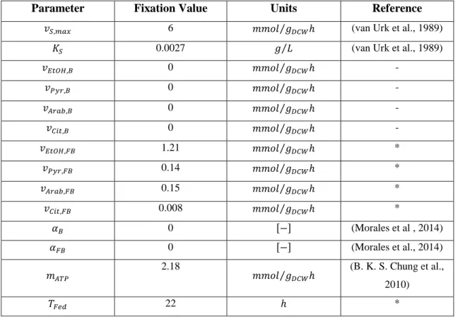
(35) 19. Where 𝑀𝐶𝐶𝑖 is the mean coefficient of confidence for dataset i, CC K the coefficient of confidence of parameter k, ni the number of parameters of the model used to fit dataset i and ∆𝐶𝐼𝑘,5% the length of the 95% Confidence Interval for the parameter k. The modeling structure of each dataset with the lowest MCC was utilized as candidate for the cross-calibration stage.. 4.5. Cross Calibration of available datasets using candidate robust modeling structures derived from the reparametrization stage. After the reparametrization of each dataset, a candidate robust modeling structure was achieved. The latter was employed to recalibrate the rest of the datasets in order to evaluate its robustness. It is worthy to note that the parameters left out of the calibration were either fixed according to values reported in literature, assumed to be zero or fixed at the mean value achieved in the calibrations. This was done in order to avoid assuming a minimum production of compounds in batch cultivations and to ensure model convergence for parameters that had no reported values in literature (feed phase consumption rates) (Table 4). We applied a maximum of 2500 iterations in the scatter search algorithm. The reduced modeling structures were evaluated according to four parameters: I.. Relative difference between objective functions (FDIFF), corresponds to the average relative difference between the objective function achieved with a reduced modeling structure in contrast to the value achieved with the original model structure. This score was determined according to the following expression: 𝑛. 𝐹𝐷𝐼𝐹𝐹. 𝐹𝑖,𝑅𝑒𝑑𝑢𝑐𝑒𝑑 − 𝐹𝑖,𝑂𝑟𝑖𝑔𝑖𝑛𝑎𝑙 1 = ∙∑ 𝑛 𝐹𝑖,𝑂𝑟𝑖𝑔𝑖𝑛𝑎𝑙. ( 19 ). 𝑖=1. Where n corresponds to the number of cultures of each type, 𝐹𝑖,𝑂𝑟𝑖𝑔𝑖𝑛𝑎𝑙 is the fit objective function for dataset i using the original model structure and 𝐹𝑖,𝑅𝑒𝑑𝑢𝑐𝑒𝑑 is.

(36) 20. the fit objective function of dataset i using a reduced, a priori robust, modeling structure.. Table 4 - Values at which problematic parameters were fixed in the cross calibration stage. Parameters marked with ‘-‘ in the reference column indicates that no a priori value was assumed for that particular parameter, which is the case for the batch minimum secretion rates. ‘*’ meant that the value of a particular parameter was fixed at the mean value achieved in the calibrations, because no information about them could be found in literature. It is worthy to mention that fixing these parameters at zero, allowed no consumption of batch by-products and yielded poor fed-batch fittings (data not shown).. Parameter. Fixation Value. Units. Reference. 𝑣𝑆,𝑚𝑎𝑥. 6. 𝑚𝑚𝑜𝑙 ⁄𝑔𝐷𝐶𝑊 ℎ. (van Urk et al., 1989). 𝐾𝑆. 0.0027. 𝑔 ⁄𝐿. (van Urk et al., 1989). 𝑣𝐸𝑡𝑂𝐻,𝐵. 0. 𝑚𝑚𝑜𝑙 ⁄𝑔𝐷𝐶𝑊 ℎ. -. 𝑣𝑃𝑦𝑟,𝐵. 0. 𝑚𝑚𝑜𝑙 ⁄𝑔𝐷𝐶𝑊 ℎ. -. 𝑣𝐴𝑟𝑎𝑏,𝐵. 0. 𝑚𝑚𝑜𝑙 ⁄𝑔𝐷𝐶𝑊 ℎ. -. 𝑣𝐶𝑖𝑡,𝐵. 0. 𝑚𝑚𝑜𝑙 ⁄𝑔𝐷𝐶𝑊 ℎ. -. 𝑣𝐸𝑡𝑂𝐻,𝐹𝐵. 1.21. 𝑚𝑚𝑜𝑙 ⁄𝑔𝐷𝐶𝑊 ℎ. *. 𝑣𝑃𝑦𝑟,𝐹𝐵. 0.14. 𝑚𝑚𝑜𝑙 ⁄𝑔𝐷𝐶𝑊 ℎ. *. 𝑣𝐴𝑟𝑎𝑏,𝐹𝐵. 0.15. 𝑚𝑚𝑜𝑙 ⁄𝑔𝐷𝐶𝑊 ℎ. *. 𝑣𝐶𝑖𝑡,𝐹𝐵. 0.008. 𝑚𝑚𝑜𝑙 ⁄𝑔𝐷𝐶𝑊 ℎ. *. 𝛼𝐵. 0. [−]. (Morales et al , 2014). 𝛼𝐹𝐵. 0. [−]. (Morales et al., 2014). 𝑚𝐴𝑇𝑃 𝑇𝐹𝑒𝑑. II.. 2.18. 22. 𝑚𝑚𝑜𝑙 ⁄𝑔𝐷𝐶𝑊 ℎ ℎ. (B. K. S. Chung et al., 2010) *. Percentage of Significance issues refers to the number of times a parameter was found to be not significantly different from zero out of the total of significance determinations performed for a particular structure. If a model structure had 6 parameters and was used to calibrate 8 datasets, 48 significance determinations were performed for that particular model.. III.. Percentage of Sensitivity issues refers to the number of times one of the estimated parameters showed no impact over state variables (average sensitivity < 0.01) for.

(37) 21. a particular modeling structure out of the total sensitivity determinations performed. IV.. Percentage of Identifiability issues, corresponds to the number of times a pair of parameters presented a strong correlation (≥ 0.95), out of the total parameter pairs of a particular modeling structure. If p is the number of parameters of the model and n is the number of datasets used for calibration, the total of parameter pairs for which identifiability was determined is: 𝑇𝑜𝑡𝑎𝑙 𝑝𝑎𝑖𝑟𝑠 =. 𝑝 ∙ (𝑝 − 1) ∙𝑛 2. ( 20 ). Finally, the modeling structure that presented the lowest FDIFF and fewest parametric problems was used as a candidate robust modeling structure for the corresponding type of culture.. 4.6. Robustness check of the chosen modeling structure Once a candidate robust modeling structure was determined for the batch and fed-batch cases, we tested its robustness (absence of parametric problems) by calibrating new experimental data. If the calibration resulted in a close fit to the data and presented no identifiability, sensitivity or significance problems, the model structure was considered like robust. For the batch model, we employed fermentation data from P. pastoris GS115 strain grown with 40 [g/L] of glucose as carbon source at T° = 25°C and pH = 6. The robustness of the fed-batch model was evaluated with a glucose-limited cultivation consisting of a 60 [g/L] of glucose batch phase and an exponential feed using 500 [g/L] of glucose. The medium was added in the feeding phase in order to achieve an exponentially decreasing growth rate from 0.1 to 0.07 [1/h]..

(38) 22. 4.7. Model validation Finally, the predicting capability of the robust batch and fed-batch models was evaluated for conditions similar to the ones used in the initial calibrations (training set). In the case of the robust batch model, we first calibrated the duplicates of the strain harboring one copy of the thaumatin gene together, obtaining a characteristic parameter set for the strain. Then, we used these parameters to predict the course of a different batch cultivation performed in the same conditions (30°C and pH 6). This procedure was also applied for the fed-batch configuration. Here, we simulated a bioreactor dynamics using the parameters obtained in the best calibration of the training dataset (the one in which the calibration objective function was minimal compared to the rest of the calibrations) using the robust modeling structure chosen previously. This prediction was compared with experimental data of a different fed-batch cultivation.. 4.8. Simulation. 4.8.1. Analysis of the metabolic flux distribution during different stages of a dynamic cultivation After the calibration of the dataset used to check the fed-batch model robustness, we extracted the flux distribution from three metabolically different stages of the cultivation in order to analyze P. pastoris’ central metabolism: i.. Exponential growth during the batch phase. ii.. Ethanol and arabitol consumption during glucose starvation. iii.. Controlled growth during the feeding phase.. In addition, we checked flux directionality against reported values and modified the genome-scale metabolic model until we observed an agreement between experimental and.

(39) 23. predicted fluxes. Finally, we recalibrated the data with the curated model and analyzed the flux distribution of P. pastoris central metabolism in the aforementioned stages.. 4.8.2. Discovery of beneficial knock-out targets for the overproduction of recombinant Human Serum Albumin To demonstrate potential applications of the model, gene targets for the overproduction of the recombinant protein Human Serum Albumin (HSA) were searched by simulating the growth and protein secretion of single knock-out strains of P. pastoris in batch cultivations. To do this, we included in the Metabolic Block a second quadratic programing problem to simulate the behavior of a knock-out strain. The second problem consisted in the Minimization of Metabolic Adjustment (MOMA) algorithm (Segrè, Vitkup, & Church, 2002), which states that, after a genetic perturbation, the cell will attempt to redistribute its metabolic fluxes as similar as possible to the parental strain (equation 22). The hypothetical parental strain was characterized using the parameters obtained in the calibration of the dataset used for the batch model validation plus a reported specific HSA productivity (qP) by P. pastoris growing in glucose (Rebnegger et al., 2014), which depended on the specific growth rate μ (). In every iteration of the model, the minimum HSA production was fixed according to this relation, which was assumed to be a third degree polynomial just of modeling purposes. Other kinetics might be used to represent the qP vs μ relation, but this depends on the strain and protein being produced (Maurer et al., 2006)..

(40) 24. qp Serum Albumin vs. μ 0,2 y = 182,52x3 - 39,406x2 + 3,1725x - 0,0271. qp [mg/gh]. 0,16 0,12 0,08 0,04 0 0. 0,02. 0,04. 0,06. 0,08. 0,1. 0,12. 0,14. 0,16. μ [h-1]. Figure 3 - Relation between Human Serum Albumin production and growth rate in a glucose limited chemostat taken from Rebnegger et al, 2014. Once the constrained model enters the metabolic block, it first solves equation 5, from which it obtains the parental flux distribution v0. Then, the k reactions associated with gene j are blocked:. 𝑙𝑏𝑙,𝑗 = 𝑢𝑏𝑙,𝑗 = 0. 𝑙 = 1…𝑘. ( 21 ). Finally, the MOMA algorithm uses the flux distribution of the parental strain v0 to calculate the knockout distribution vKO as the Euclidean distance between them, considering that the actual model has the corresponding deletion. MOMA: 𝑀𝑖𝑛 (𝑣0 − 𝑣𝐾𝑂,𝑗 ) 𝑠. 𝑡. 𝑆 ∙ 𝑣𝐾𝑂,𝑗 = 0. 2. ( 22 ).

(41) 25. 𝑙𝑏𝑖 ≤ 𝑣𝑖,𝐾𝑂,𝑗 ≤ 𝑢𝑏𝑖. 𝑖 = 1…𝑛. We performed one batch simulation for every gene in the model, which were evaluated in terms of final protein and biomass concentrations and compared its performance against the parental strain. The candidates that reached a higher HSA concentration than the parental strain were manually analyzed and some of them were proposed as candidates to improve HSA production.. 4.8.3. Evaluation of different feeding policies in silico to improve recombinant protein production considering specific information about the strain and process setup We also evaluated feeding policies to improve the volumetric productivity of HSA production, considering information about a strain of interest and process limitations. Simulations were performed using the parameters obtained in the calibration of the fedbatch validation dataset and including HSA biosynthesis in the mass balances. We used the same volumetric productivity (qP) vs growth rate (μ) relation from (Rebnegger et al., 2014) to determine protein production as a function of the growth rate. The process limitations (based in our setup) were a maximum reactor volume of 1 L, and a maximum oxygen transfer rate of 10.9 [g/L·h], given by a k La of 300 h-1 and a driving force of (CO2,SATURATION – CO2,SETPOINT) of 36.2 [mg/L], considering the incorporation of pure oxygen into the bioreactor. If any of these thresholds were violated by either the feeding rate of medium or the oxygen uptake rate (extracted from the model), the integration stopped. We evaluated 13 exponential feeding policies. Five of them maintained a constant growth rate during the feeding phase and the rest considered a decreasing growth rate throughout the culture (Supplementary Material 3). After the simulation, we ranked the strategies according to the volumetric productivity of recombinant HSA and chose the best one as a culture alternative that could potentially improve bioreactor performance..

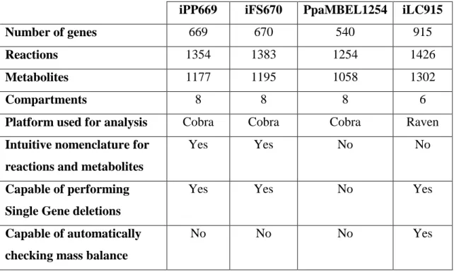
(42) 26. 5.. RESULTS AND DISCUSSION. 5.1. Genome-Scale model selection from literature The main components and the relevant usability features of published GSMs of Pichia pastoris are detailed in Table 5. The PpaMBEL1254 model was discarded due to the lack of intuitive reaction and metabolite names, as well as the absence of gene-protein relations (at least in the online version), hampering the analysis of knock-out strains. All the models share the same structure of the central metabolism, which carries most of the flux entering the cell.. Table 5 - Main components and usability features of available genome-scale metabolic models of Pichia pastoris. iPP669. iFS670. PpaMBEL1254. iLC915. Number of genes. 669. 670. 540. 915. Reactions. 1354. 1383. 1254. 1426. Metabolites. 1177. 1195. 1058. 1302. 8. 8. 8. 6. Platform used for analysis. Cobra. Cobra. Cobra. Raven. Intuitive nomenclature for. Yes. Yes. No. No. Yes. Yes. No. Yes. No. No. No. Yes. Compartments. reactions and metabolites Capable of performing Single Gene deletions Capable of automatically checking mass balance. After the determination of the average relative error between model predictions and experimental data (Carnicer et al., 2009; Solà et al., 2007) (Table 6), we selected the iFS670 model since it has a desirable structure and better reproduces experimental data from P. pastoris chemostats. It is worth mentioning that the inclusion of the arabitol.

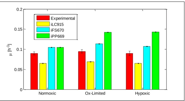
(43) 27. biosynthesis pathway into Chung’s (iPP669) model – resulting in the iFS670 model greatly improved the predictions of specific growth rate, Oxygen Uptake Rate (OUR) and Carbon Dioxide Evolution Rate (CER) in hypoxic glucose-limited chemostats (Supplementary Material 1). Specifically, the deviation of carbon towards arabitol reduced the predicted growth rate in those conditions when compared to the iPP669 model (Figure 4), resulting in a reduction of the difference with the corresponding experimental value.. Table 6 - Average error of model predictions using two datasets from carbon-limited chemostats. In glyceroland/or methanol (MetOH) – limited chemostats, the models were employed to predict specific growth rate µ, Oxygen Uptake Rate (OUR) and carbon dioxide evolution rate (CER) in four different conditions, which gives a total of 12 predictions. In the glucose limited chemostats, the models were used to estimate µ, OUR, CER, ethanol secretion rate and arabitol secretion rate in six conditions, which gives a total of 30 model predictions. Experimental data was taken from (Carnicer et al., 2009; Solà et al., 2007). Carbon Source. iLC915. iFS670. iPP669. Number of predictions. Glycerol/MetOH. 78%. 37%. 38%. 12. Glucose. 85%. 36%. 52%. 30. Overall Error (F). 83%. 36%. 48%. 42. Figure 4 - Experimental and model-predicted specific growth rates using glucose as the only carbon source at different oxygen levels for a P. pastoris wild type strain. Data taken from (Carnicer et al., 2009). 0.2. -1  [h ]. 0.15. Experimental iLC915 iFS670 iPP669. 0.1. 0.05. 0. Normoxic. Ox-Limited. Hypoxic.

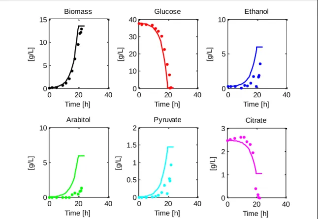
(44) 28. 5.2. Batch model development In this section, we present the steps followed to achieve a robust dFBA modeling structure of aerobic batch cultures of Pichia pastoris, capable of fitting new data with as few parametric problems as possible and predicting bioreactor dynamics.. 5.2.1. Initial calibration The initial structure of the batch model (eight parameters) was capable of fitting different cellular dynamics from eight aerobic batch cultivations (Figure 5 and Supplementary Material 5). 10 Concentration [g/L]. 30 Biomass. 20. Glucose 10 0. Dissolved Oxygen Concentration [mg/L]. Ethanol. 0. 5. 10 15 Time[h]. 20. 10. Arabitol 6 4 2. 0. 5. 10 15 Time[h]. 20. 25. 20. 25. 4. 8 6 4 2 0. 8. 0. 25. Concentration [g/L]. Concentration [g/L]. 40. 0. 5. 10 15 Time[h]. 20. 25. Pyruvate. 3. Citrate 2. 1. 0. 0. 5. 10 15 Time[h]. Figure 5 - Model calibration of a glucose-limited aerobic batch cultivation of Pichia pastoris. Experimental data from two replicates is shown with points and the model fit is presented in continuous lines. Also, the dissolved oxygen profile (in [mg/L]) is included in the bottom left graph..

(45) 29. Production of ethanol and arabitol was detected in the cultivations, which was probably caused by the high initial glucose concentration used in the experiments. Ethanol production during batch cultivations has already been reported (Heyland et al., 2010), however, the formation of these compounds has usually been associated to oxygen scarcity in glucose-limited conditions (Baumann et al., 2010; Carnicer et al., 2009). The mean, minimum and maximum values of the model parameters, calculated for the calibrations, are presented in Table 7. Results show that the initial fittings covered a wide range of values. Here, the suboptimal growth parameter alpha (αB) was always greater than zero, which indicates that the model “prefers” to include the minimization of total fluxes in the objective function, rather than only maximizing specific growth rate. This forces the metabolic block to solve a QP problem, which has the practical benefit of eliminating redundant cycles in the resulting flux distributions, also called Type III Pathways (Price, Famili, Beard, & Palsson, 2002), - which make metabolic pathway analyses cumbersome.. Table 7 - Minimum, Mean and Maximum parameter values achieved in batch model calibrations. More details on the calibrations can be found in Supplementary material 5.. Parameter. Minimum. Mean. Maximum. Units. 𝑉𝑀𝐴𝑋. 1,27. 4,286. 7,948. [mmol/gDCW·h]. 𝐾𝑆. 1e-05. 2,96E-04. 9,80E-04. [g/L]. 𝑣𝐸𝑡𝑂𝐻,𝐵. 0,024. 1,363. 2,968. [mmol/gDCW·h]. 𝑣𝑃𝑦𝑟,𝐵. 0,003. 0,145. 0,248. [mmol/gDCW·h]. 𝑣𝐴𝑟𝑎𝑏,𝐵. 0,088. 0,373. 0,541. [mmol/gDCW·h]. 𝑣𝐶𝑖𝑡,𝐵. 1e-05. 0,177. 1,104. [mmol/gDCW·h]. 𝛼𝐵. 1,454e-06. 2,17E-04. 4,15E-04. [-]. 𝑚𝐴𝑇𝑃. 0,001. 3,064. 10,000. [mmol/gDCW·h].