Classification and modeling of time series of astronomical data

Texto completo

(1)Pontificia Universidad Católica de Chile Facultad de Matemáticas Departamento de Estadı́stica. Classification and Modeling of time series of astronomical data por Felipe Elorrieta López Tesis presentada al Departamento de Estadı́stica de la Pontificia Universidad Católica de Chile para optar al grado de Doctor en Estadı́stica. Octubre, 2018. Director de Tesis: Dr. Susana Eyheramendy Duerr c ⃝Copyright por Felipe Elorrieta López, 2018.

(2) FACULTAD DE MATEMÁTICAS PONTIFICIA UNIVERSIDAD CATÓLICA DE CHILE. INFORME DE APROBACIÓN TESIS DE DOCTORADO. Se informa a la Facultad de Matematı́cas que la Tesis de Doctorado presentada por el candidato Felipe Elorrieta López ha sido aprobada por la Comisión de Evaluación de la Tesis como requisito para optar al grado de Doctor en Estadı́stica, en el examen de Defensa de Tesis rendido el dı́a 12 de Octubre de 2018.. Director de Tesis Dr. Susana Eyheramendy Duerr Comisión de Evaluación de la Tesis Dr. Wilfredo Palma Manriquez Dr. Giovanni Motta Dr. Pablo Estevez Dr. Cristian Meza.

(3) FACULTAD DE MATEMÁTICAS PONTIFICIA UNIVERSIDAD CATÓLICA DE CHILE. Fecha: 12 de Octubre 2018. Autor. :Felipe Elorrieta López. Tı́tulo Departamento Grado Convocación. :Classification and Modelling of time series of astronomical data :Estadı́stica :Doctor :Octubre 2018. Se le concede permiso para hacer circular y copiar, con propósitos no comerciales, el tı́tulo ante dicho para los requerimientos de individuos y/o instituciones.. Firma del Autor. EL AUTOR SE RESERVA LOS DERECHOS DE OTRAS PUBLICACIONES, Y NI LA TESIS NI EXTRACTOS EXTENSOS DE ELLA, PUEDEN SER IMPRESOS O REPRODUCIDOS SIN EL PERMISO ESCRITO DEL AUTOR. EL AUTOR ATESTIGUA QUE EL PERMISO SE HA OBTENIDO PARA EL USO DE CUALQUIER MATERIAL COPYRIGHTED QUE APAREZCA EN ESTA TESIS (CON EXCEPCIÓN DE LOS BREVES EXTRACTOS QUE REQUIEREN SOLAMENTE EL RECONOCIMIENTO APROPIADO EN LA ESCRITURA DEL ESTUDIANTE) Y QUE TODO USO ESTÉ RECONOCIDO CLARAMENTE..

(4) ii. Acknowledgments Un dı́a de marzo de 2014, empezó esta aventura de más de cuatro años. En este momento, cuando al fin entrego mi trabajo de tesis de Doctorado, quiero agradecer a todas las personas que fueron de vital importancia para lograr este objetivo. En primer lugar, quiero agradecer a mi compañera de vida Milka Vescovi, por todo él apoyo y paciencia durante todo este tiempo. Te Amo. A mis hijos Iñigo y Julián por darme la fuerza para no flaquear con los inconvenientes que se presentaron en el camino. A mi madre Jovita López por la formación que me llevo a lograr este objetivo, a mi hermano Pablo Elorrieta por el desinteresado apoyo durante todos mis años de estudio, a mi hermano mayor Gonzalo Elorrieta y a mi padre Julio Elorrieta, que se que habrı́a estado muy orgulloso de este logro y su eterno recuerdo sigue siempre presente en mi. Además, quiero agradecer a mi profesora Guı́a Susana Eyheremandy, en primer lugar por la carta de recomendación para la postulación al programa de Doctorado en Estadı́stica y a la Beca Conicyt. Luego, por darme la oportunidad de desarrollar este tema de Tesis y por toda la orientación entregada durante estos cuatro años. Al profesor Wilfredo Palma, por su crucial apoyo para sacar este tema adelante. A los profesores de la comisión evaluadora por los comentarios realizados, los cuales ayudaron a hacer de este un mejor trabajo. Al profesor Reinaldo Arellano, por guiar mi tesis de Magister y recomendarme al programa de Doctorado en Estadı́stica y a la Beca Conicyt. Finalmente, quisiera hacer una mención especial al profesor Francisco Torres, quien me incentivó a tomar la decisión de seguir el camino del Doctorado en Estadı́stica. Este trabajo está dedicado a su memoria. También, a todos los que fueron parte de mi vida durante estos años. A Francisca y Carolina por brindarme su apoyo y asistir a mi exposición de defensa de grado. A mis amigos de la USACH Eto, Ruy y Diego que pese a las pocas veces que nos reunimos, cada una de ellas fue una inyección de energı́a para terminar este trabajo. Finalmente, quiero agradecer el apoyo del Instituto Milenio de Astrofisica (MAS) y a la Beca de Doctorado CONICYT No. 21140566..

(5) Contents List of Figures. vii. List of Tables. xiii. 1. Introduction xvii 1.1 Purpose of the study . . . . . . . . . . . . . . . . . . . . . . . . . . . . . xx 1.1.1 General objective . . . . . . . . . . . . . . . . . . . . . . . . . . xx 1.1.2 Specific objectives . . . . . . . . . . . . . . . . . . . . . . . . . xx. 2. Literature Review 2.1 Astronomical Background . . . . . . . . . . . . 2.1.1 Light curves . . . . . . . . . . . . . . . 2.1.2 Variable Stars . . . . . . . . . . . . . . . 2.1.3 Astronomical Surveys . . . . . . . . . . 2.2 Time Series Background . . . . . . . . . . . . . 2.2.1 Analysis in Time Domain . . . . . . . . 2.2.2 Analysis in Frequency Domain . . . . . . 2.3 Machine Learning Background . . . . . . . . . . 2.3.1 The General Classification Problem . . . 2.3.2 State-of-the-art Data Mining Algorithms . 2.3.3 Measuring classifier performance . . . .. 3. . . . . . . . . . . .. . . . . . . . . . . .. . . . . . . . . . . .. . . . . . . . . . . .. . . . . . . . . . . .. . . . . . . . . . . .. . . . . . . . . . . .. . . . . . . . . . . .. Light Curves Classification 3.1 Light-curve extraction and pre-processing . . . . . . . . . . . . 3.2 Feature Extraction of Light Curves . . . . . . . . . . . . . . . . 3.2.1 Periodic Features . . . . . . . . . . . . . . . . . . . . . 3.2.2 Non-Periodic Features . . . . . . . . . . . . . . . . . . 3.3 A Machine Learned Classifier for RR Lyrae in the VVV Survey 3.3.1 RRab classification in the VVV . . . . . . . . . . . . . 3.3.2 Classification Procedure . . . . . . . . . . . . . . . . . 3.3.3 Training sets . . . . . . . . . . . . . . . . . . . . . . . iii. . . . . . . . . . . .. . . . . . . . .. . . . . . . . . . . .. . . . . . . . .. . . . . . . . . . . .. . . . . . . . .. . . . . . . . . . . .. xxiii . xxiii . xxiv . xxv . xxvii . xxxi . xxxi . xxxix . xliii . xliii . xliii . lii. . . . . . . . .. lv lvi lviii lix lx lxiii lxiii lxiv lxv. . . . . . . . ..

(6) iv. 3.4. 3.5. 3.3.4 Choice of classifier . . . . . . . . . . . . . . . . . . . Optimization of Classification Algorithms . . . . . . . . . . . 3.4.1 Choice of aperture for photometry . . . . . . . . . . . 3.4.2 Feature selection . . . . . . . . . . . . . . . . . . . . 3.4.3 Sensitivity to training set choice . . . . . . . . . . . . 3.4.4 Final classifier . . . . . . . . . . . . . . . . . . . . . Performance on independent datasets . . . . . . . . . . . . . . 3.5.1 RRab in 2MASS-GC 02 and Terzan 10 . . . . . . . . 3.5.2 RRab in the outer bulge area of the VVV . . . . . . . 3.5.3 Census of RRab stars along the southern galactic disk.. . . . . . . . . . .. . . . . . . . . . .. . . . . . . . . . .. . . . . . . . . . .. . . . . . . . . . .. . . . . . . . . . .. lxvi lxvii lxx lxxiv lxxv lxxvi lxxvii lxxviii lxxix lxxxi. 4. Light Curves Modeling lxxxv 4.1 Irregular Autoregressive (IAR) model . . . . . . . . . . . . . . . . . . . lxxxv 4.1.1 Estimation of IAR Model . . . . . . . . . . . . . . . . . . . . . lxxxviii 4.1.2 IAR Gamma . . . . . . . . . . . . . . . . . . . . . . . . . . . . lxxxix 4.1.3 Simulation Results . . . . . . . . . . . . . . . . . . . . . . . . . xc 4.2 Complex Irregular Autoregressive (CIAR) model . . . . . . . . . . . . . xciv 4.2.1 State-Space Representation of CIAR Model . . . . . . . . . . . . xcvi 4.2.2 Estimation of CIAR Model . . . . . . . . . . . . . . . . . . . . . xcix 4.2.3 Simulation Results . . . . . . . . . . . . . . . . . . . . . . . . . c 4.2.4 Comparing the CIAR with other time series models . . . . . . . . c 4.2.5 Computing the Autocorrelation in an Harmonic Model . . . . . . cii 4.3 Application of Irregular Time Series Models in Astronomical time series . civ 4.3.1 Irregular time series models to detect the harmonic model misspecification . . . . . . . . . . . . . . . . . . . . . . . . . . . . cvii 4.3.2 Statistical test for the autocorrelation parameter . . . . . . . . . . cxi 4.3.3 Irregular time series models to detect multiperiodic variable stars cxii 4.3.4 Classification Features estimated from the irregular time series models . . . . . . . . . . . . . . . . . . . . . . . . . . . . . . . cxv 4.3.5 Exoplanet Transit light-curve . . . . . . . . . . . . . . . . . . . . cxvii 4.4 AITS Package in R . . . . . . . . . . . . . . . . . . . . . . . . . . . . . cxviii 4.4.1 The gentime function . . . . . . . . . . . . . . . . . . . . . . . . cxx 4.4.2 The harmonicfit function . . . . . . . . . . . . . . . . . . . . . . cxx 4.4.3 The foldlc function . . . . . . . . . . . . . . . . . . . . . . . . . cxxi 4.4.4 Simulating the Irregular Time Series Processes . . . . . . . . . . cxxi 4.4.5 Fitting the Irregular Time Series Processes . . . . . . . . . . . . cxxii 4.4.6 Testing the significance of the parameters of the irregular models . cxxvii. 5. Discussion cxxxi 5.1 Future Works . . . . . . . . . . . . . . . . . . . . . . . . . . . . . . . . cxxxiv.

(7) v A Connection Between CAR(1) and IAR process. cxlv.

(8) vi.

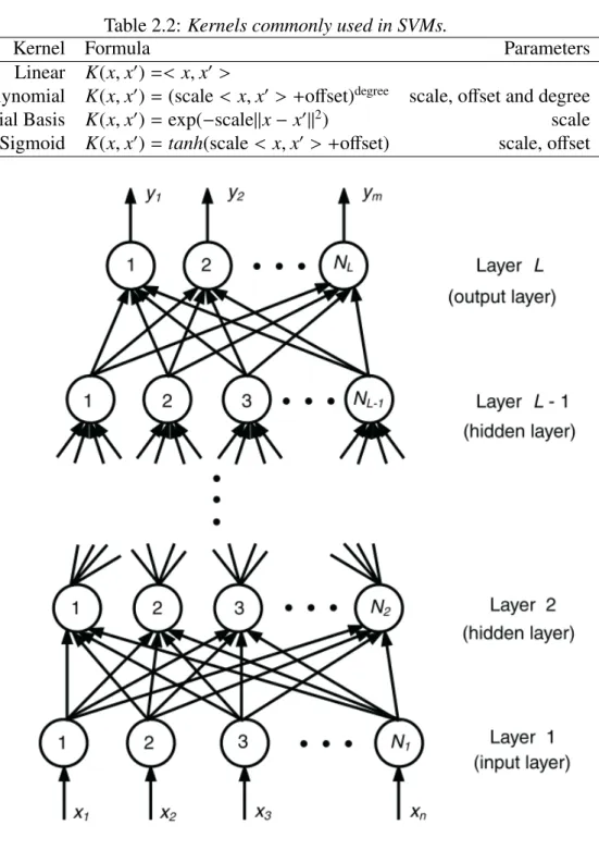
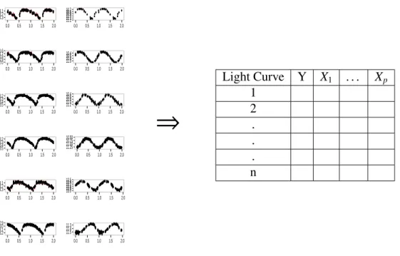
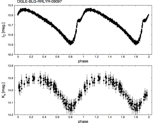
(9) List of Figures 1.1. Statistical challenges in the light curves analysis addressed in this work .. xx. 2.1. ‘Variability tree’ showing the many different types of stellar (and nonstellar) phenomena that are found in astronomy, (from Eyer & Mowlavi, 2008 [29]). . . . . . . . . . . . . . . . . . . . . . . . . . . . . . . . . . xxvi. 2.2. 2MASS map of the inner Milky Way showing the VVV bulge (solid box, −10o < l < +10o and −10o < b < +5o ) and plane survey areas (dotted box, −65o < l < 10o and −2o < b < +2o ), (from Minniti, 2010 [48]). . . . xxix. 2.3. VVV Survey Area Tile Numbers Galactic Coordinates (from Catelan et al. 2013 [17]). . . . . . . . . . . . . . . . . . . . . . . . . . . . . . . . . xxix. 2.4. Workflow of Ensemble Methods (from Utami, et al., 2014) [72]. . . . . . xlv. 2.5. Illustration of the optimal hyperplane in SVC for a linearly separable (from Meyer, 2001) [47]. . . . . . . . . . . . . . . . . . . . . . . . . . . xlix. 2.6. Illustration of multi-layer feed-forward networks (from Zhang, 2000) [75].. 3.1. a) Original light curve of an RRab star observed in B295 field folded in its period. b) Light curve of the RRab star after the elimination of one observation with large magnitude error . c) Light curve of the RRab star after the elimination of two outliers observations. . . . . . . . . . . . . . lvii. 3.2. Illustration of the process in which each light curve in the training set is represented as a vector of features. . . . . . . . . . . . . . . . . . . . . . lviii. 3.3. a) Folded light curve of an RRab star with R1 = 0.46 observed in B295 field of the VVV. b) Folded light curve of an RRab star with R1 = 0.77 observed in B295 field of the VVV . c) Folded light curve of a variable star with R1 = 1.18 observed in B295 field of the VVV. . . . . . . . . . .. l. lxi. 3.4. Example of a known RRab classified by OGLE using an optical IC light curve (upper panel). It shows a very symmetric light curve in the infrared (lower panel, K s light curve from the VVV). . . . . . . . . . . . . . . . . lxiv. 3.5. Flowchart of the classifier building phase. . . . . . . . . . . . . . . . . . lxv vii.

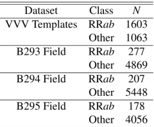
(10) viii 3.6. 3.7. 3.8. 3.9 3.10 3.11 3.12. 3.13. 3.14 3.15. Optimization of the number of variables in each tree (mtry parameter) used in Random Forest. In Figure a) is the F-Measure (y-axis) computed for values of the mtry parameter (x-axis) when all the features are used in the classifier. In Figure b) is the F-Measure (y-axis) computed for values of the mtry parameter (x-axis) when only the 12 selected features are used in the classifier. . . . . . . . . . . . . . . . . . . . . . . . . . . . . . . . lxix Optimization of parameters of Multi Hidden Neural Network. On the left figure is the F-Measure (y-axis) computed for number of Hidden Layers used in the Neural Network (x-axis). On the right figure is the F-Measure (y-axis) computed for the Batch Size used in the Neural Network (x-axis). lxx Optimization of the number of iterations used in the data mining algorithms implemented this work. The red line is the F-Measure computed for Random Forest, the yellow line corresponds to Stochastic Boosting, the green line is for the Deep Neural Network, the light blue line is for the multi hidden neural network. Finally, the blue, violet and pink lines corresponds to the AdaBoost algorithm with coeflearn Breiman, Freund and Zhu respectively. In figure a) the 12 selected features are used and the minError strategy of aperture selection in each classifier. In figure b) all the features are used and the KDC strategy of aperture selection. In figure c) the 12 selected features are used and the KDC strategy of aperture selection. . . . . . . . . . . . . . . . . . . . . . . . . . . . . . . . . . . lxxi Number of light curves with the minimum sum of squared errors at each aperture size. . . . . . . . . . . . . . . . . . . . . . . . . . . . . . . . . lxxii Kernel density estimates of the mean magnitude of curves with the minimum sum of squared errors at each aperture size. . . . . . . . . . . . . . lxxiii Feature importance using the Ada.M1 classifier. Based on this graph, we chose to consider only the 12 most important features in the final classifier. lxxv Histogram of scores obtained by the classifier for the light curves of the sample presented by Alonso-Garcı́a et al. [2]. Shown are the true positives (sources classified by Alonso-Garcı́a et al. [2] as RRab), false positives, and false negatives. . . . . . . . . . . . . . . . . . . . . . . . . . . . . . lxxviii Two sources that were nominally false positives: (a) Terzan10 V113; (b) internal identifier 273508. One of them (a) is a bona fide false positive, while the other (b) is a true positive that was not flagged as such in the work of Alonso-Garcı́a et al. [2] (see text). . . . . . . . . . . . . . . . . lxxix Light curves of RRab stars found by Gran et al. (2016) in the outer bulge area of the VVV which were confirmed by the classifier. . . . . . . . . . lxxx Histogram of scores obtained by the classifier for the outer bulge lightcurves of the sample used by Gran et al. (2016). Shown are the true positives (sources classified by as RRab), false positives, and false negatives.lxxxi.

(11) ix 3.16 Kernel Density estimation of the classification score for RRab (green density) and No RRab (red density) and overall (green density). The blue and black lines correspond to the contamination and precision respectively (from Dekany et al, 2018 [25]). . . . . . . . . . . . . . . . . . . . . . . . lxxxii 4.1. Simulated IAR Time Series of length 300 and ϕ = 0.9. . . . . . . . . . . lxxxvi. 4.2. Comparison of standard deviation of innovations computed using the IAR model and other time series models that assumes regular times. The red line is the standard deviation of the data, the blue and green lines are the standard deviation of innovations computed using the AR(1) and ARFIMA(1,d,0) model respectively. The black line is the mean of the standard deviation of innovation computed using the IAR(1) model. . . . xciii. 4.3. Comparison of root mean squared error at each time of a sequence simulated with the IAR model with parameter ϕR = −0.99, ϕI = 0, c = 0 and length n = 300. The red line corresponds to the standard deviation of the sequence, the blue, green, gray and orange lines correspond to the RMSE computed when the sequence was fitted with IAR(1), AR(1), ARMA(2,1), CAR(1) models respectively. The black line corresponds to the root mean squared error of the CIAR model, where the black dots are the individual RMSE at each time. . . . . . . . . . . . . . . . . . . . . .. cii. 4.4. In the first row are shown on figures (a) and (b) the kernel Distributions of the root mean squared error computed for the fitted models on the 1000 CIAR sequences simulated. In a) each CIAR process was generated using ϕR = −0.99. In b) each CIAR process was generated using ϕR = 0.99. The other parameters of the models were defined as ϕI = 0, c = 0 and length n = 300. In the second row are shown on figures (c) and (d) the RMSE computed for different values of the autocorrelation parameter ϕR of the CIAR model. The red, blue, green, darkgreen and black lines correspond to the RMSE computed for the CIAR, IAR, AR, ARFIMA and CAR models respectively. In Figure (c) the observational times are generated using a mixture of Exponential distribution with λ1 = 15 and λ2 = 2, ω1 = 0.15 and ω2 = 0.85. In figures (a), (b) and (d) the observational times are generated using a mixture of Exponential distribution with λ1 = 130 and λ2 = 6.5, ω1 = 0.15 and ω2 = 0.85. . . . . . . . . . . . . . . . . . . . . ciii. 4.5. Estimated coefficients (y-axis) by the CIAR model in k = 200 harmonic processes generated using frequencies (x-axis) in the interval (0, π). The black line corresponds to the coefficients estimated by the CIAR model. The red line is the theoretical autocorrelation of the process yti . . . . . .. 4.6. cv. Values of the coefficient estimated by the CIAR and IAR models in OGLE and HIPPARCOS light curves. . . . . . . . . . . . . . . . . . . . . . . . cvi.

(12) x 4.7. Kernel Density of the RMSE computed for the residuals of harmonic fit in the light curves when the CIAR coefficient is negative. The red density corresponds to the RMSE computed using the IAR model, and the green density corresponds to the RMSE computed using the CIAR model. . . . cvii. 4.8. Boxplot of the distribution of ϕ, for the light-curves using the correct frequency (on the left) and for the light-curves using the incorrect frequency (on the right). . . . . . . . . . . . . . . . . . . . . . . . . . . . . . . . . cix. 4.9. In the first row, the light curves of a Classical Cepheid, EW and DSCUT are shown on figures (a)-(c) respectively. The continuous blue line is the harmonic best fit. On the second row (figures (d)-(f)), for each of the variable stars, it is depicted on the x-axis the % of variation from the correct frequency, and on the y-axis is the estimate of the parameter ϕ of the IAR model obtained after fitting an harmonic model with the wrong period (except at zero that corresponds to the right period). On the third row (figures (g)-(i)), the distribution of the parameter ϕ of the IAR model is shown when each light curve is fitted with the wrong period. The red triangle corresponds to the value of ϕ when the correct period is used in the harmonic model fitting the light curves. . . . . . . . . . . . . . . . .. cx. 4.10 a) Light curve of a RRc star observed by the HIPPARCOS survey. The continuous blue line is the harmonic best fit. b) Logarithm of the absolute value of the estimated parameter ϕˆR by the CIAR model on the residuals of the harmonic model fitted with different frequencies. In the x-axis are the percentual variation from the correct frequency, in the y-axis are the logarithm of ϕ̂. c) Logarithm of the estimated parameter ϕ̂ by the IAR model on the residuals of the harmonic model fitted with different frequencies. In the x-axis are the percentual variations from the correct frequency, in the y-axis is the logarithm of ϕ̂. . . . . . . . . . . . . . . . cxii 4.11 a) Light curve of a RRab star observed by the VVV survey. The continuous blue line is the harmonic best fit. b) Logarithm of the absolute value of the estimated parameter ϕˆR by the CIAR model on the residuals of the harmonic model fitted with different frequencies. In the x-axis are the percentual variation from the correct frequency, in the y-axis are the logarithm of ϕ̂. c) Logarithm of the estimated parameter ϕ̂ by the IAR model on the residuals of the harmonic model fitted with different frequencies. In the x-axis are the percentual variations from the correct frequency, in the y-axis is the logarithm of ϕ̂. . . . . . . . . . . . . . . . . . . . . . . . cxiii 4.12 (a) Residuals of the best harmonic fit with one frequency for a simulated multiperiodic light curve; (b) Residuals of the best harmonic best fit with two frequencies for the same simulated multiperiodic light curve. . . . . . cxiv.

(13) xi 4.13 In the first column are shown on figures (a) and (c) the residuals after fitting an harmonic model with one period for two double mode Cepheids. On the second column (figures (b) and (d)), the residuals of the same variable stars after fitting an harmonic model with two periods are shown. 4.14 a) Boxplot of the ϕR and the p-value estimated from the CIAR model in the RR-Lyraes variable stars separated by subclasses. b) Boxplot of the ϕR and the p-value estimated from the CIAR model in the Cepheids variable stars separated by subclasses. . . . . . . . . . . . . . . . . . . . . . . . 4.15 (a) Residuals after fitting the model for a transiting exoplanet; (b) The red triangle represents the log(ϕ̂), where ϕ̂ is the parameter of the IAR model. The black line represents the density of the ϕ for the randomized experiment. . . . . . . . . . . . . . . . . . . . . . . . . . . . . . . . . . 4.16 Simulated IAR Time Series of length 300 and ϕ = 0.9. The times was generated by the mixture of exponential distributions with parameters λ1 = 130, λ2 = 6.5, ω1 = 0.15 and ω2 = 0.85. . . . . . . . . . . . . . . . 4.17 Figure a) shows the time series of the Simulated IAR-Gamma Process with length 300 and ϕ = 0.9. The times was generated by the mixture of exponential distributions with parameters λ1 = 130, λ2 = 6.5, ω1 = 0.15 and ω2 = 0.85. Figure (b) shows the histogram of the IAR-Gamma observations . . . . . . . . . . . . . . . . . . . . . . . . . . . . . . . . 4.18 Real part of the simulated CIAR process of length 300, ϕR = 0.9, ϕI = 0.9 and the nuisance parameter c = 1. The times was generated by the mixture of exponential distributions with parameters λ1 = 130, λ2 = 6.5, ω1 = 0.15 and ω2 = 0.85. . . . . . . . . . . . . . . . . . . . . . . . . . . 4.19 Figure a) shows the Density Plot of the log(ϕ), where ϕ was estimated by the IAR model when the time series is fitted using wrong periods. The red triangle is the log(ϕ) estimated when the correct period is used in the harmonic fit. Figure (b) shows the same plot for the CIAR process. . . .. cxvi. cxvii. cxix. cxxiii. cxxv. cxxvii. cxxix.

(14) xii.

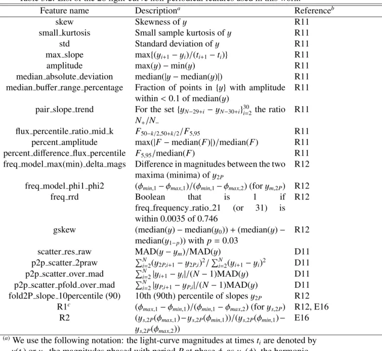
(15) List of Tables 2.1 2.2 2.3 3.1 3.2 3.3 3.4 3.5 3.6 3.7 3.8 4.1. 4.2 4.3. 4.4. 4.5. Most common pulsating variable stars and their amplitudes (in tude) and periods (in days) (from Eyer & Mowlavi, 2008 [29]). Kernels commonly used in SVMs. . . . . . . . . . . . . . . . . Activation functions commonly used in MLP. . . . . . . . . . .. magni. . . . . xxvii . . . . . l . . . . . li. List of the 40 light-curve periodical features used in this work. . . . . . . lx List of the 28 light-curve non-periodical features used in this work. . . . . lxii Number of RRab versus other classes in the training datasets. . . . . . . . lxvi State-of-the-art data mining algorithms used to build the classifier for RRab.lxvii Cross-validation performance of classifiers on the templates+B293+B294+B295 training set, using all features . . . . . . . . . . . . . . . . . . . . . . . . lxviii F1 Measure by Aperture and Classifier Algorithm . . . . . . . . . . . . . lxxiii Cross-validation performance of classifiers on the templates+B293+B294+B295 training set, using the best 12 features . . . . . . . . . . . . . . . . . . . lxxiv F-measure by training set (Adaboost.M1) . . . . . . . . . . . . . . . . . lxxvi Maximum likelihood estimation of simulated IAR series with mixture of Exponential distribution for the observational times, with λ1 = 130 and λ2 = 6.5, ω1 = 0.15 and ω2 = 0.85. . . . . . . . . . . . . . . . . . . . . Maximum likelihood estimation of simulated IAR series of size n, with Exponential distribution mix observation times, λ1 = 300 and λ2 = 10. . Implementation of IAR and CAR models on simulated Gamma-IAR series in R and Python. For the observational times we use a mixture of two Exponential distributions with parameters λ1 = 130 and λ2 = 6.5, w1 = 0.15 and w2 = 0.85. . . . . . . . . . . . . . . . . . . . . . . . . . . . . Maximum likelihood estimation of complex ϕ computed by the CIAR model in simulated IAR data. The observational times are generated using a mixture of Exponential distribution with λ1 = 15 and λ2 = 2, w1 = 0.15 and w2 = 0.85. . . . . . . . . . . . . . . . . . . . . . . . . . . . . . . . Distribution of the forty selected examples by his frequency range and class of variable stars. . . . . . . . . . . . . . . . . . . . . . . . . . . . .. xiii. xci xci. xcii. ci cviii.

(16) Classification and Modeling of time series of astronomical data. Abstract We are living in the era of Big Data, where several tools have been developed to deal with large amount of data. These technological advances have allowed the rise of the astronomical surveys. These surveys are capable to take observations from the sky and from them generate information ready to be analyzed. Among the observations available there are light curves of astronomical objects, such as, variable stars, transients or supernovae. Generally, the light curves are irregularly measured in time, since it is not always possible to get observational data from optical telescopes. This issue makes the light curves analysis an interesting statistical challenge, because there are few statistical tools to analyze irregular time series. In addition, due to the large amount of light curves available in each survey, automated processes are also required to analyze all the information efficiently. Consequently, in this thesis two goals are addressed: the classification of the light curves from the implementation of data mining algorithms and the temporal modeling of them. Regarding the classification of light curves, our contribution was to develop a classifier for RR Lyrae variable stars in the Vista Variables in the Via Lactea (VVV) nearinfrared survey. It is important to detect RR-Lyraes since they are essential to build a three-dimensional map of the Galactic bulge. In this work, the focus is on RRab type ab (i.e., fundamental-mode pulsators). The final classifier is built following eight key steps that include the choice of features, training set, selection of aperture, and family of classifiers. The best classification performance was obtained by the AdaBoost classifier which achieves an harmonic mean between false positives and false negatives of ≈ 7%. The performance is estimated using cross validation and through the comparison with two independent datasets that were classified by human experts. The classifier implemented has already made it possible to identify some RRab in the outer bulge and the southern galactic disk areas of the VVV. In addition, I worked on modeling light curves. I develop new models to fit irregularly spaced time series. Currently there are few tools to model this type of time series. One example is the Continuous Autoregressive model of order one, CAR(1), however some assumptions must be satisfied in order to use this model. A new alternative to fit irregular time series, that we call the irregular autoregressive model (IAR model), is proposed. The IAR model is a discrete representation of the CAR(1) model which provide more flexibility, since it is not limited by Gaussian time series. However, both the CAR(1) and IAR model are only able to estimate positive autocorrelations. In order to fit negatively correlated irregular time series a Complex irregular autoregressive model (CIAR model) was also developed. For both models maximum likelihood estimation procedures are proposed. Furthermore, the finite sample performance of the parameters estimation is assessed by Monte Carlo simulations. Finally, for both models some applications are proposed on astronomical data. Applications include the detection of multiperiodic variable.

(17) xv stars and the verification of the correct estimation of the parameters in models commonly used to fit astronomical light curves. Keywords: light curves, variable stars, RR-Lyrae, irregular time series, autoregressive models, data mining algorithms..

(18) xvi.

(19) Chapter 1 Introduction In the era of Big Data, Astronomy is undergoing a major revolution. Due to the advances in technology the astronomical surveys have evolved from taking observations of small and focused areas of the sky (for example OGLE [68] and HIPPARCOS [28]) to widefield surveys (for example VVV [48]). The Large Synoptic Survey Telescope (LSST) is one of the upcoming big challenge in astronomy. It will take a full picture of the whole sky every three nights. This survey is designed to conduct a ten-year survey of the dynamic universe, from 2022 - 2032. This project will generate a huge amount of data posing important challenges that require the expertise from diverse disciplines such as for example Statistics, Informatics and Astronomy. All this data will be available to the community of astronomers living in Chile. Therefore, in order to face the challenges of the LSST, the Millennium Institute of Astrophysics (MAS) was created. The MAS has gathered over a hundred researchers and students from five prestigious Chilean Universities. The MAS is divided into five research lines, where one of them is Astrostatistics & Astroinformatics. The role of astro-statisticians is to provide models and tools to process large datasets and extract valuable knowledge from them. For example, data mining and machine learning algorithms will allow us to automate processes necessary to analyze all fields observed by a specific astronomical survey in a short time. Some astronomical data available for statistical analysis are light curves, which represent the temporal variations of the brightness of an astronomical object. The light curves can represent the brightness of variable stars, the transit of an extrasolar planet or a supernovae. Light curves analysis offers many astronomical and statistical challenges. For astronomers, light curves analysis allow to study the dynamic properties of an xvii.

(20) xviii object. For example, light curves can differ in the degree of change in magnitude, in the degree of regularity from one cycle to the next and in the length of the cycle (period). These properties can be related to physical properties of the system, like rotation and binary period. These dynamic properties allow the astronomers, for example, to identify the class of a specific variable star only by inspecting the temporal behavior of a star. For statisticians, light curves consist on a time series of the brightness variation of stars. Generally, this time series are irregularly measured in time, since it is not always possible to get observational data from optical telescopes, because its dependency, for example, on clear skies. Working with irregular time series is an important statistical challenge because there are still few robust statistical tools to analyze unequally spaced time series. Some examples are in the estimation of the spectrum of an irregular time series using the Lomb-Scargle periodogram (Zechmeister & Kürster 2009) [74]) or the continuous-time autoregressive moving average (CARMA) models to fit irregular time series (Kelly et al. (2014) [43]). In this thesis my focus is to provide new methods to analyze light curves of variable stars. This is performed following two approaches, the classification of light curves from the implementation of data mining algorithms and the temporal modeling of them. The challenges that will be addressed in both approaches are shown in Figure 1.1. Regarding the classification of variable stars, the main aim is to build automated procedures to classify pulsating variable stars from the VVV survey, such as RR Lyraes and Cepheids. The basic idea is that the classifiers that are implemented must be useful for the astronomers in the process of searching pulsating stars within the VVV observation area. Finding pulsating variable stars in the VVV is particularly interesting, since they are essential to determine the three-dimensional structure of our Galaxy. In order to build the classifier, I followed the procedure proposed by Debosscher et al. (2007) [23], Dubath et al. (2011) [26], Richards et al. (2011) [56]. The basic idea is to compute characteristics or features of the variable stars from an harmonic model fitted to them. Later, the set of features computed for the variable stars in the training set are used as input in the supervised data mining algorithms. Some additional aims in the classifier construction were addressed. First, to provide new features specifically designed to better characterize the temporal behavior of the pulsating classes. Second, the data mining algorithm used generally for classification problems in Astronomy is the Random Forest. I looked for an alternative from a wide variety of state-of-the-art data mining algorithms..

(21) xix Another purpose of this thesis, is to provide new methods to the modeling of irregular time series. Currently, the light curves are fitted using the CARMA family of models. Particularly, using the CAR(1) model is possible to estimate the autocorrelation of a irregularly sampled time series. However, the CAR(1) model have some assumptions, e.g., Gaussian distribution and continuous white noise. In this work, a more flexible alternative to fit irregularly sampled time series is introduced. This model is called the irregular autoregressive model (IAR model), which is a discrete representation of the CAR(1) model. This model is more flexible than the CAR(1) model, since it allows non-Gaussian distributed data. Furthermore, both CAR(1) and IAR models are only able to estimate positive autocorrelation. That is a limitation compared to the regular autoregressive model which can detect both positive and negative time dependencies. In order to address this constraint, a second model, called the complex irregular autoregressive model (CIAR), is proposed. This model is an extension of the irregular autoregressive model that allows to estimate both positive and negative autocorrelation. In this work, these models are applied in the analysis of astronomical light curves. The light curves are generally modeled using a parametric model that assumes independent and homoscedastic errors. However, these assumptions are not necessarily satisfied, since in many cases there remain a temporal dependency structure on the errors. Here the aim of the irregular time series models is to verify whether the parametric model is capable to describe all the temporal structure of the light curves. Consequently, in this thesis we present automated and efficient computational methods under a solid statistical framework applied to solve common problems in the analysis of astronomical data. The structure of this thesis is as follows. In the following section of this chapter the purpose of the study is given. In Chapter 2 the literature on both astronomy and statistical background is reviewed, putting the main emphasis in describing the machine learning algorithms and the methods used currently to model irregular time series. In Chapter 3 I describe the procedure to build a machine learning classifier for the light curves of variable stars. This procedure is presented in eight key steps. The first half corresponds with the data cleaning and the feature extraction steps. The second half of the procedure corresponds to the implementation of two different classifiers, one for the RRab and other for the Cepheids. In both cases, the optimization of machine learning algorithms, the selection of the most important features and assessing the performance of the trained classifier are presented, putting some emphasis in the challenges to build each classifier in the VVV..

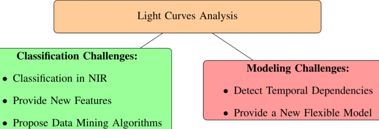
(22) xx. Light Curves Analysis. Classification Challenges: • Classification in NIR • Provide New Features • Propose Data Mining Algorithms. Modeling Challenges: • Detect Temporal Dependencies • Provide a New Flexible Model. Figure 1.1: Statistical challenges in the light curves analysis addressed in this work. In Chapter 4 we present new and flexible methods to model the irregular time series, which are the irregular autoregressive model (IAR) and the Complex irregular autoregressive model (CIAR). In both cases the estimation procedure is described. In addition, the performance of the maximum likelihood estimators is assessed via Monte Carlo simulations. Some applications in astronomical data of both models are also presented. Finally, in Chapter 5, the conclusions and future works are drawn.. 1.1 1.1.1. Purpose of the study General objective. Provide statistical methods with a robust framework to analyze efficiently a large number of light curves for astronomical data observed using surveys such as OGLE, HIPPARCOS and the VVV.. 1.1.2. Specific objectives. 1. To build an automated procedure to classify RR Lyrae type ab stars from the VVV survey. 2. To assess the performance of the classifier on different datasets in which flux measurements do not necessarily follow the same conditions in cadence, depth, etc. as our training set..

(23) xxi 3. To propose an irregular autoregressive time series model to detect time dependencies on the light curves of astronomical data under a solid statistical framework. 4. To extend the irregular autoregressive model to allow the data to come from other statistical distributions and to detect negative time dependencies..

(24) xxii.

(25) Chapter 2 Literature Review 2.1 Astronomical Background Since mankind look at the sky for the first time we have tried to find an explanation to the mysteries of the universe. Over the course of thousand years of our history several scientists, e.g., Aristotle, Nicolaus Copernicus, Johannes Kepler, Galileo, Isaac Newton and Albert Einstein have made significant contributions to explain the astronomical phenomena. These contributions start in the third century when Aristotle believed that the Earth was at the center of the universe. Later Copernicus proposed that the Sun, not the Earth, was the center of the Solar System. In the early 1600s, Kepler proposed three laws that describe the motion of planets around the Sun. Galileo was the first to use systematically a telescope to observe celestial objects, this allows him to discover the phases of Venus. Sir Isaac Newton improves the Kepler laws of motion and developed the theory of universal gravity. Finally, Einstein developed the theory of general relativity in 1915, which describes how mass and space are related to each other. This theory has been fundamental to better understand astronomical phenomena such as the black holes. All these contributions have allowed us to better understand how the universe works. Nowadays, we live in the era of the astronomical surveys. Due to the availability of powerful computers, these surveys are capable to take observations from the sky and from them generate a great amount of information ready to be analyzed by the astronomers. Several scientists from different areas have been attracted by this large amount of information available. Consequently, in this era networks of interdisciplinary collaboration have been created in order to analyze all the available data. These networks are generally composed by astronomers, statisticians, informatics and other related scientists.. xxiii.

(26) xxiv All this available data allows us to study and detect patterns of several astronomical objects that are of interest like the stars, planets, supernovas and other variables phenomena. The statistical challenge here, is to provide methods that allow us to analyze efficiently the available information. Particularly, in this work are addressed two main issues. First, the implementation of an automated procedure to classify variable stars in the VVV survey. The most important challenge related to the classifier is to propose a data mining procedure that considers steps of data cleaning, data transformation and assessment of the implemented classification models. In addition, it is important to test alternative classification methods to the well-known Random Forest algorithm, commonly used to address this problem. Secondly, the modeling of astronomical time series is another important topic to address. In astronomy it is common to find irregular time series because some conditions must be met to take observations of the sky. Nowadays, there are few methods for modeling irregularly sampled time series. In this work has been made a contribution in this sense, providing new models to fit irregularly sampled time series. The details of each method will be discussed in the following chapters of this thesis. However, some important concepts must be explained previously.. 2.1.1. Light curves. Astronomical observations are taken from a region of the sky. From each region observations are obtained several times, which produces a sequence of images in time. Photometry is the technique of astronomy that allows precise measurement of the brightness of an astronomical object from an image. Historically, several methods have been used to perform the photometry. The last revolution in this sense, came with the rise of the CCD technology. Using photometry on a sequence of images taken for an astronomical object, a temporal sequence of the brightness measurements can be obtained. This time sequence of brightness measurements is called the light curve of the astronomical object. Consequently, we can define the light curve as a time series of its brightness variations. The light curve allows to follow the behavior of a specific astronomical object through the time. Additionally, we can define the apparent magnitude as the brightness of an object as it appears to you. Changes in magnitude are in logarithmic scale, i.e., each magnitude means factor of 2.512 in brightness, according to a brightness ranking, originally devel-.

(27) xxv oped by Hipparchos (140 AD). Generally, the light curves are plotted using the apparent magnitude in axis y and the Julian date in axis x. If the astronomical object is periodic, and the period is known, it becomes useful to plot a phased light curve. The phase ϕ of an observation can be computed as, ( ) t − t0 ϕ= − E(t) (2.1.1) p where t0 is the reference time, t is the time when the observation was taken, p is the period of the light curve and E(t) is the integer part of t−tp 0 , sometimes called as the epoch. The phase generally is expressed as the fraction of the star cycle, taking values in the interval [0,1].. 2.1.2 Variable Stars A variable star is a star whose brightness magnitude fluctuates. Historically, variable stars have been the main tool for determining the content and structure of stellar systems and have had a crucial role in the history of Astronomy. Among these stars, we can differentiate two types depending on whether the process creating the observed variability is inherent to the star (intrinsic variation) or not (extrinsic variation.) The General Catalog of Variable Stars (Samus et al. 2009 [58]) lists over 110 classes and subclasses based on a variety of criteria. In Figure 2.1 is shown a ‘Variability tree’ (from Eyer & Mowlavi, 2008 [29]), which gives a visual summary of several of the different types of variable phenomena that may be found in astronomy, in this diagram four division levels are introduced. In the first level are the “classical” division between extrinsic and intrinsic variables. In the second level a distinction is made according to the type of object, being either asteroids, stars, or galaxies. The third level identifies the phenomenon at the origin of the variability. In the group with extrinsic variability, the phenomena considered are the rotation, microlensing effects and eclipses by a companion or by a foreground object. Among the former, are the eclipsing binaries. The eclipsing binaries are a system in which two stars orbiting a common center of mass. This type of variable stars is composed by the classes Ellipsoidal (ELL), Beta Persei (EA), Beta Lyrae (EB) and the W Ursae Maj (EW). Among the intrinsic variable objects one finds the eruptive variables, the cataclysmic variables, the rotational variables and finally the pulsating variables. Arguably the most.

(28) xxvi important group among the intrinsic variables is that of pulsating variables because it contains the RR Lyrae and Cepheids classes, which satisfy a relation between their periods and absolute luminosities that allow to estimate distances, a quantity both fundamental and elusive in Astronomy. For a current review of the physics and phenomenology of pulsating stars, we refer to the recent monograph by Catelan & Smith (2015) [16].. Figure 2.1: ‘Variability tree’ showing the many different types of stellar (and non-stellar) phenomena that are found in astronomy, (from Eyer & Mowlavi, 2008 [29]). Many classes of variable stars can also be divided into subclasses. For example, the RR-Lyraes are divided between RR Lyrae types ab and c (sometimes alternatively termed RR0 and RR1, respectively) if the stars pulsate in the fundamental radial mode or in the first-overtone radial mode respectively. The main difference between these subclasses of RR-Lyrae is that the RRab have longer pulsation periods and asymmetric light curves, while the RRc have shorter pulsation periods and almost sinusoidal light curves. The Cepheids can also be divided in the Classical Cepheids (Type I) and the Type II. The different Cepheids types obey different period-luminosity relations. In general, Type I Cepheids are brighter than Type II Cepheids, if both have the same period..

(29) xxvii In addition, it is well known that the Cepheids and RR-Lyraes have multi-periodic subclasses such as DMCEP (Double-Mode Cepheid) and RRD (Double-Mode RR-Lyrae) respectively (Moskalik, 2014 [49]). Table 2.1 shows a briefly description of the most common variable stars with its respective observational properties,. Table 2.1: Most common pulsating variable stars and their amplitudes (in magnitude) and periods (in days) (from Eyer & Mowlavi, 2008 [29]). Class name Period (Days) Amplitude (mag) Cepheids 2-70 0.1-1.5 RR Lyrae 0.2-1.1 0.2-2 SR-MIRA 50-1000 up to 8 SPB 0.5-5 up to 0.03 RVTau 30-150 1-3 δ-Scuti 0.02-0.25 up to few 0.1 As mentioned in the previous chapter, in this thesis most of the analysis will be done on the light curves of variable stars, so it is very important to have cleared these concepts to understand the subsequent results. The data of the light curves of several stars (variables and non-variables) can be extracted from different astronomical surveys. In this work the information sources that will be used are the OGLE, HIPPARCOS and the VVV survey whose characteristics will be described below.. 2.1.3 Astronomical Surveys 2.1.3.1. OGLE and HIPPARCOS Survey. The Optical Gravitational Lensing Experiment (OGLE) is a ground-based survey from Las Campanas Observatory covering fields in the Magellanic Clouds and Galactic bulge. The OGLE survey began regular sky monitoring on April 12, 1992 as one of the firstgeneration microlensing sky surveys. The project is now in its fourth phase. The first phase of the project (OGLE-1) started in 1992 (Udalski et al, 1992 [67]) and observations were continued for four consecutive observing seasons through 1995. The OGLE-II survey collected data from January 1997 to December 2000 (Udalski et al, 1997 [68]). On June 12, 2001 regular observations of the OGLE-III phase began (Udalski 2003b) and ended in May 2009. Finally, the OGLE-IV survey began regular observations of the sky on the night of March 4/5, 2010 (Udalski et al, 2015 [69])). Since 1997 observations have been conducted with the modern automated 1.3 m Warsaw telescope at the Las Campanas Observatory, Chile..

(30) xxviii Throughout the 25-year history of OGLE it has been discovered hundreds of thousands of pulsating stars. Most of the observations are collected in the I-band filter with a number of collected epochs between 120-150 in OGLE-IV (Udalski, 2017 [70]). Hipparcos (The High Precision Parallax Collecting Satellite) Space Astrometry Mission (Perryman et al. 1997 [28]) was an ESA project designed to precisely measure the positions of more than one hundred thousand stars. Launched in August 1989, Hipparcos successfully observed the celestial sphere for 3.5 years before operations ceased in March 1993. Among the 118218 stars measured by Hipparcos, 11597 were found to be (possibly) variable. Of these more than 8000 were new.. 2.1.3.2. VVV ESO Public Survey. The Vista Variables in the Via Lactea (VVV) is an ESO public survey that is performing a variability survey of the Galactic bulge and part of the inner disk using ESO’s Visible and Infrared Survey Telescope for Astronomy (VISTA), a 4m-class telescope operated by ESO and located at Cerro Paranal, Chile. The VISTA Telescope has started the observations in February 2010 and has finished in October 2015, in this time it took 1929 hours of observation. The sky area covered by the survey was of 520 deg2 (Fig.1 2.2), where there are 109 point sources, an estimated ∼ 106 − 107 variable stars, 33 known globular clusters and approximately 350 open clusters. Unlike optical surveys such as OGLE and HIPPARCOS, the VVV is characterized by using near-infrared filters (Z, Y, J, H and Ks) (NIR). The size of an uniformly covered field (also called a “tile”) is 1,501 deg2 , hence the VVV Survey requires a total of 348 such “tiles” to cover the survey area (see (Fig 2.3)), a total of 196 tiles are needed to map the bulge area and 152 tiles for the disk. Aperture photometry of VVV sources is performed on single detector frame stacks provided by the VISTA Data Flow System (Irwin et al. 2004 [39]) of the Cambridge Astronomy Survey Unit (CASU). A series of flux-corrected circular apertures are used as detailed in previous publications (Catelan et al. 2013 [17]; Dekany et al. 2015 [24]). The smallest√5 apertures, which we denoted as 1, 2, 3, 4, 5, are extracted in aperture radii of √ {0.5, 1/ 2, 1, 2, 2} arcsec. The final products will be a deep NIR atlas in five passbands. One of the main goals is to gain insight into the inner Milky Way origin, structure, and evolution. This will be achieved, for instance, by obtaining a precise three-dimensional map of the Galactic bulge. To achieve this goal, the pulsating stars like Cepheids or RR-Lyrae are of particular importance, for example, there are many RR Lyrae in the direction of the bulge and,.

(31) xxix. Figure 2.2: 2MASS map of the inner Milky Way showing the VVV bulge (solid box, −10o < l < +10o and −10o < b < +5o ) and plane survey areas (dotted box, −65o < l < 10o and −2o < b < +2o ), (from Minniti, 2010 [48]).. Figure 2.3: VVV Survey Area Tile Numbers Galactic Coordinates (from Catelan et al. 2013 [17]). because they are very old, they are fossil records of the formation history of the Milky Way. For a detailed account of the VVV see Minniti et al. (2010) [48], and for a recent status updated with emphasis on variability see Catelan et al. (2014) [18]. With the information extracted from the VVV, OGLE and HIPPARCOS surveys, catalogues of known variable stars have been created, which will be useful to test the classifi-.

(32) xxx cation and modeling methods that will be proposed in this work. The main idea is to have previously certified tools that allows us to be prepared when future synoptic studies such as the Large Scale Synoptic Telescope (LSST, Ivezic et 2008 [40]) become operational. The Large Synoptic Survey Telescope (LSST) is the upcoming big challenge in astronomy, this survey is designed to conduct a ten-year survey of the dynamic universe from 2022 - 2032. Among its main goals is to define more precisely the structure and formation of our home galaxy, the Milky Way and cataloging the solar system..

(33) xxxi. 2.2 Time Series Background In the study of astronomical data, the time series tools have been widely used to explain the temporal behavior of the flux of astronomical objects such as, variable stars, transients or supernovae. This is useful since these objects can be characterized from its temporal behavior. For example, from a suitable time series model, can be derived a set of features able to distinguish between different types of variable stars. The astronomical observations are generally obtained at irregular time gaps due to some conditions must be met to be able to observe in the optical telescopes, for example, that the sky is clear. This implies several statistical challenges because there are few statistical tools specifically developed to work with unequally spaced time series. A time series can be defined as a real valued sequence of observations Yn with n = 1, . . . , N measured in observational times tn such that the sequence t1 , . . . , tN is strictly increasing. A time series is called regular if the distance of consecutive times t j − t j−1 is constant, whereas if this distance is not constant, the time series is called irregular. Another basic distinction can be made between the time series tools depending on the domain in which they operate. First the time domain methods will be reviewed.. 2.2.1 Analysis in Time Domain First, I will introduce some basic ideas of the time series analysis. Among the most important concepts in time series are the following: • Strict stationarity: A stochastic process Yt is strictly stationary (or strongly stationary) if each joint distribution F of a finite sequence of length n (Y1 , Y2 , . . . , Yn ) is invariant to a translation in k times, i.e., F(Yk+1 , Yk+2 , . . . , Yk+n ) = F(Y1 , Y2 , . . . , Yn ) ∀n, k ∈ Z • Weak stationarity: A stochastic process Yt is weakly stationary (or second-order stationarity) if, 1. E[Yt ] = µ < ∞ ∀t ∈ T 2. V[Yt ] = σ2 < ∞ ∀t ∈ T 3. There exists a function γ(.) such that Cov(Yt , Y s ) = γ(t − s) ∀t, s ∈ T.

(34) xxxii It is easy to check that if Yt is strictly stationary and E(Yt2 ) < ∞ ∀t then Yt is also weakly stationary [11]. • Autocovariance function Let Yt be a weakly stationary process. The autocovariance function (ACVF) of Yt at lag k is, γ(k) = Cov(Yt , Yt−k ) • Autocorrelation function The autocorrelation function (ACF) of Yt at lag k is, ρ(k) =. γ(k) γ(0). • White Noise A weakly stationary sequence ϵt is called white noise if all observations of this sequence are uncorrelated. If the mean of ϵt are 0 then the sequence can be denoted ϵt ∼ WN(0, σ2 ). Time series models can be implemented under two scenarios. When the observations are measured regularly or irregularly in time. The basic time series processes are defined in the regular case. The most common model used to fit a weakly stationary time series is the ARMA(p,q) model.. 2.2.1.1. ARMA Models. Yt is an ARMA(p,q) process, if Yt is weakly stationary and can be written as, Yt − ϕ1 Yt−1 − . . . − ϕ p Yt−p = ϵt + θ1 ϵt−1 + . . . + θq ϵt−q. (2.2.1). where ϵt ∼ WN(0, σ2 ). In addition, let Φ(B) = (1 − ϕ1 B − . . . − ϕ p B p ) and Θ(B) = (1 + θ1 B + . . . + θq Bq ) the autoregressive polynomial and the moving-average polynomial respectively. The process is well defined if Φ(B) and Θ(B) have no common factors. A condition for which a stationary solution of 2.2.1 exists is that the zeros of the autoregressive polynomial Φ(B) = (1 − ϕ1 B − . . . − ϕ p B p ) are located outside of the unit circle. Some particular cases of the ARMA models can be defined, for example, • Autoregressive process (AR). If Yt is an ARMA(p,q) process with q = 0, then Yt ∼ AR(p) and can be written as, Yt − ϕ1 Yt−1 − . . . − ϕ p Yt−p = ϵt. (2.2.2).

(35) xxxiii • Moving-Average process (MA). If Yt is an ARMA(p,q) process with p = 0, then Yt ∼ MA(q) and can be written as, Yt = ϵt + θ1 ϵt−1 + . . . + θq ϵt−q. (2.2.3). The ARMA(p,q) process can be estimated by maximum likelihood. Let the observations equally spaced on time Y = (Y1 , . . . , Yn )′ have a Gaussian distribution, with the follow covariance matrix, Γλ = (γ(i − j))ni, j=1 = (Cov(Yi , Y j ))ni, j=1 with λ = (ϕ1 , . . . , ϕ p , θ1 , . . . , θq , σ2 )′ is the parameter vector of the model. The likelihood of Y is, { } 1 ′ −1 −n/2 −1/2 L(λ) = (2π) |Γλ | exp − Y Γλ Y 2 . From Section 5.2 of Brockwell and Davis [11] the maximum likelihood estimator λ̂ is asymptotically normal.. 2.2.1.2. ARFIMA Models. The ARMA model is a particular case of the general linear process. Another particular class of linear time series is called long memory processes. On the contrary of the ARMA models, the long-memory processes are characterized by an autocovariance function not absolutely summable, i.e. , the autocovariance function γ(k) is such that, ∞ ∑. |γ(k)| = ∞. k=−∞. A well-known class of long-memory models is the autoregressive fractionally integrated moving-average (ARFIMA) processes. An ARFIMA process Yt may be defined by, Φ(B)Yt = Θ(B)(1 − B)−d ϵt. (2.2.4). where Φ(B) and Θ(B) are the autoregressive polynomial and the moving-average polynomial respectively. In addition, (1 − B)−d is a fractional differencing operator defined by the binomial expansion, −d. (1 − B). =. ∞ ∑ j=0. η jBj. (2.2.5).

(36) xxxiv where ηj =. Γ( j + d) Γ( j + 1)Γ(d). for d < 12 , d , 0, −1, −2, . . . and ϵt is a white noise sequence with finite variance. If the process (2.2.4) satisfy that d ∈ (−1, 12 ), and the polynomials Φ(B) and Θ(B) have no common zeros, then the stationarity, causality and invertibility of an ARFIMA model can be established. Each time series model reviewed previously may be represented in many different forms. Some examples are the Wold expansion, the autoregressive expansion and the state space systems. Here, I will focus in the state-space system, since it will be very useful later on.. 2.2.1.3. State-Space Systems. A linear state space system may be described by the following equations, Xt = Ft−1 Xt−1 + Vt−1. (2.2.6). Yt = GXt + Wt. (2.2.7). where (2.2.6) is known as the state equation which determines a v−dimensional state variable Xt and the second equation (2.2.7) is called the observation equation, which expresses the w−dimensional observation Yt . In addition, Ft is a sequence of v × v called the transition matrix, G ∈ Rw×v is the observation linear operator of the observation matrix. Finally, Wt ∼ WN(0, Rt ), Vt ∼ WN(0, Qt ) and Vt is uncorrelated with Wt . Properties • Stability A state space system is said to be stable if Ftn converges to zero as n tends to ∞. If λ is an eigenvalue of Ft associated to the eigenvector x, then Ftn x = λn x. Thus, if the eigenvalues of Ft satisfy |λ| < 1 then λn → 0 as n increases. Consequently, F n x also converges to zero as n → ∞. In the stable case the equations (2.2.9) have the unique stationary solution given by Xt =. ∞ ∑ j=0. Ftj Vt− j−1.

(37) xxxv The corresponding sequence of observations. Y t = Wt +. ∞ ∑. GFtj Vt− j−1. j=0. is also stationary. • Hankel Matrix. ∑ Suppose that ψ0 = 1 and ψ j = GF j−1 ∈ R for all j > 0 such that ∞j=0 ψ2j < ∞. Then from (2.2.6)- (2.2.7), the process Yt may be written as the Wold expansion Yt =. ∞ ∑. ψ2j ϵt− j. j=0. This linear process can be characterized by the Hankel matrix given by     H =   .  ψ1 ψ2 ψ3 . . .   ψ2 ψ3 ψ4 . . .   ψ3 ψ4 ψ5 . . .  .. .. .. ..  . . . .. Since the state space representation of a linear regular process is not necessarily unique, one may ask what the minimal dimension of the state vector is. In order to answer this question it is necessary to introduce the concepts of observability and controllability. • Observability Let O = (G′ , Ft′G′ , Ft′2G′ , . . .)′ be the observability matrix. The system (2.2.6)(2.2.7) is said to be observable if and only if O is full rank or, equivalently, O′ O is invertible. The definition of observability is related to the problem of determining the value of the unobserved initial state x0 from a trajectory of the observed process {y0 , y1 , . . .} in the absence of state or observational noise..

(38) xxxvi • Controllability Consider the case where the state error is written in terms of the observation so that Vt = HWt and the state space model can be expressed as,. Xt+1 = Ft Xt + HWt. (2.2.8). Yt = GXt + Wt. (2.2.9). Let C = (H, Ft H, Ft2 H, . . .) be the controllability matrix. The system (2.2.8)- (2.2.9) is controllable if C is full rank or, C′ C is invertible. • Minimality A state space system is minimal if Ft is of minimal dimension among all representations of the linear process (3.3). A state space system is minimal if and only if it is observable and controllable.. The estimation of the state space models can be performed by the following Kalman recursive equations. For the state-space model (2.2.6)- (2.2.7), the one-step predictors X̂t = Pt−1 (Xt ) and their error covariance matrices Σt = E[(Xt − X̂t )(Xt − X̂t )′ ] are unique and determined by the initial conditions X̂1 = P(X1 |Y0 ),. Σ1 = E[(X1 − X̂1 )(X1 − X̂1 )′ ]. And the recursions, for t = 1, . . . Λt = Gt ΩtG′t + Rt. (2.2.10). Θt = Ft ΩtG′t. (2.2.11). ′ Ωt+1 = Ft Ωt Ft′ + Qt − Θt Λ−1 t Θt. (2.2.12). νt = Yt − Gt X̂t. (2.2.13). X̂t+1 = Ft X̂t + Θt Λ−1 t νt. (2.2.14). where {νt } is called the innovation sequence. The optimization of the parameters in Kalman recursion was made by minimizing the reduced likelihood defined as,.

(39) xxxvii ) n ( νt2 1∑ ℓ(ϕ) ∝ log(Λt ) + n t=1 Λt So far, I have introduced the methods to analyze regular time series. Suppose now a sequence of observational times and values (tn , Yn ) such that the series t1 , . . . , tN is strictly increasing and the distance between consecutive times, t j − t j−1 is not constant ∀ j = 1, . . . , N, i.e., henceforth it will be assumed that Y1 , . . . , YN was irregularly measured in time. Generally, when a time series is measured in continuous time, the notation changes slightly, writing Y(t) rather than Yt . An usual approach to fit irregular time series is using the continuous-time autoregressive moving average (CARMA) models 2.2.1.4. CARMA Models. Continuous-time ARMA processes are defined in terms of stochastic differential equations analogous to the difference equations that are used to define discrete-time ARMA processes. The continuous time AR(1) (CAR (1)) process is defined as a stationary solution of the first-order stochastic differential equation. d Y(t) + α0 Y(t) = σν(t) + β (2.2.15) dt where ν(t) is the continuous time white noise, α0 and β are unknown parameters of the model. In addition, ν(t) = dtd B(t), where B(t) is the standard Brownian motion or Wiener process. The derivative of B(t) does not exist in the usual sense, so equation (2.2.15) is interpreted as an Itô differential equation, dY(t) + α0 Y(t)dt = σdB(t) + βdt,. t > 0,. (2.2.16). with dY(t) and dB(t) denoting the increments of Y and B in the interval (t, t + dt) and Y(0) a random variable with finite variance, independent of {B(t)}. The solution of (2.2.16) can be written as, ∫ t ∫ t −α0 t −α0 (t−u) Y(t) = e Y(0) + σ e dB(u) + β e−α0 (t−u) du 0. 0. or equivalently, Y(t) = e. −α0 t. Y(0) + e. −α0 t. I(t) + βe. −α0 t. ∫ 0. t. eα0 u du. (2.2.17). ∫t where I(t) = σ 0 eα0 u dB(u) is an Itô integral satisfying E(I(t)) = 0 and Cov(I(t+h), I(t)) = ∫t σ2 0 e2α0 u du for all t ≥ 0 and h > 0. It can be shown that necessary and sufficient conditions for {Y(t)} to be stationary are α0 > 0, E(Y(0)) = β/α0 and V(Y(0)) = σ2 /(2α0 ). In addition, under these conditions.

(40) xxxviii. E(Y(t)) = β/α0 Cov(Y(t + h), Y(t)) =. σ2 −α0 h e 2α0. ( ) Further, if Y(0) ∼ N β/α0 , σ2 /(2α0 ) , then the CAR(1) process is also Gaussian and strictly stationary. If a > 0 and 0 ≤ s ≤ t, it follows from (2.2.17) that Y(t) can be expressed as, Y(t) = e−α0 (t−s) Y(s) +. ) β ( 1 − e−α0 (t−s) + e−α0 t (I(t) − I(s)) α0. (2.2.18). or equivalently, ( ) β β −α0 (t−s) Y(t) − =e Y(s) − + e−α0 t (I(t) − I(s)) α0 α0. (2.2.19). We can be extending the model (2.2.15) to a standard continuous time autoregressive model of order (p) (CAR(p)) process {Y(t)}: D p Y(t) + α1 D p−1 Y(t) + . . . + α p Y(t) = β0 DB(t). (2.2.20). It is useful to represent this equation in operator notation as α(D)Y(t) = B(t) where, α(D) = D p + α1 D p−1 + . . . + α p−1 D + α p. (2.2.21). A parameterization used by Jones (1981) [41] was based on the zeros r1 , . . . , r p of α(D) such that α(D) =. p ∏. (D − ri ). i=1. The necessary and sufficient condition for the stationarity of the model is that all the zeros have negative real parts. In Belcher et al, (1994) [6] it is defined a new parameterization, where the old parameters αi may be constructed from the new parameters ϕi . The link between the α and ϕ parameters is given by,. β(D) = β0 D p + β1 D p−1 + . . . + β p−1 D + β p =. p ∑. ϕi (1 − D/κ)i (1 + D/κ) p−i. (2.2.22). i=0. where κ is a scale parameter and we take ϕ0 = 1. Thus the βi are linear combinations of the ϕi . Now let α(s) = β(s)/β0 so that αi = βi /β0 . In a CAR(1) model we can prove that (1+ϕ1 ) α1 = κ (1−ϕ . The function car of the R packages cts ([73]) estimates the reparametrized 1).

(41) xxxix autoregressive parameters ϕi . Finally, we define a zero-mean CARMA(p,q) process {Y(t)} (with 0 ≤ q < p) to be a stationary solution of the pth-order linear differential equation, D p Y(t) + α1 D p−1 Y(t) + . . . + α p Y(t) = β0 DB(t) + β1 D2 B(t) + . . . + βq Dq+1 B(t) (2.2.23) where D( j) denotes j-fold differentiation with respect to t. Since the derivatives D j B(t), j > 0, do not exist in the usual sense, we interpret (2.2.23) as being equivalent to the state-space system. As mentioned above, the time series methods can be distinguished according to the domain in which works. As the methods which works in time domain were already revised, now the methods that operate in the frequency domain will be seen. Here also the distinction between regular and irregular time series will be made.. 2.2.2 Analysis in Frequency Domain Frequency-domain methods are based in the discrete Fourier transform. The main difference with the time-domain analysis is that these methods are based on the correlation function, while the Frequency-domain methods analyze the response of the process to given set of frequencies. This type of analysis is also called spectral analysis.. 2.2.2.1. Spectral Analysis in regular case. Let ω denote the frequency, such that −π < ω < π, and let P denote the period, such that P = 2π . Given a time series {Yt }, the spectrum is defined to be the Fourier transform of ω the autocovariance function γy (h) fy (ω) =. ∞ 1 ∑ −ihω e γy (h) 2π h=−∞. Now, if we know the spectrum fy (ω), from Herglotz Theorem we can compute γy (h) using the inverse Fourier transform: ∫π γy (h) =. eihω fy (ω)dω −π. These results show that the Fourier spectrum can be directly mapped onto the timedomain autocovariance function, in this sense the frequency and time domain methods.

(42) xl are closely related. To estimate the spectral density, we may compute the periodogram, which is defined as the squared modulus of the discrete Fourier transform of the autocovariance function, i.e., 2 ∞ 1 ∑ −ihω I(ω) = e γy (h) 2π h=−∞. A sampled data set like 2πn j with j = . . . , −3, −2, −1, 0, 1, 2, 3, . . . contains complete information about all spectral components in a signal Yt , between the low fundamental frequency 2π and the high Nyquist frequency π. n Fourier analysis has restrictive assumptions, for example, equally spaced time series and sinusoidal shaped variations. As mentioned above, these assumptions are rarely achieved in real astronomical data. There are several methods more appropriate to use in this context, as for example the Lomb Scargle Periodogram.. 2.2.2.2. Lomb-Scargle Periodogram. The Lomb-Scargle (LS) periodogram is an extension of the conventional periodogram for unevenly sampled time series. For a time series (ti , Yi ) with zero mean, the normalized LS periodogram can be computed as,  N  N ∑  ∑ 2 2 [ yi sin(ωti − τ)]   [ yi cos(ωti − τ)]  1  i=1 i=1   PLS (ω) = +  N N  ∑ 2σ2  ∑ 2  cos2 (ωti − τ) sin (ωti − τ)  i=1. i=1. where ω = 2π f is the angular frequency, f is the ordinary frequency, τ is the phase and σ2 is the sample variance of yi . The parameter τ is defined by, N ∑. tan(2ωτ) =. sin(2ωti ). i=0 N ∑. cos(2ωti ). i=0. Lomb (1976) [45] showed that PLS is identical to the least-squares fit of a single component stationary sinusoidal model of the form y(t) = A sin(ωt + τ). Consequently, the dominant angular frequency ω is the value that best fit the time series in a least squares sense. This frequency also corresponds to the maximum power in the Lomb-Scargle periodogram. The sinusoidal model can also be expressed by y(t) = a cos(ωt) + b sin(ωt).

(43) xli where the √ amplitude A and the phase ψ can be computed from the estimated parameters as A = a2 + b2 and ψ = atan(a/b) respectively. However, the Lomb-Scargle periodogram have two shortcomings. First, this method assumes that the mean of the data is equivalent to the mean of the fitted sine functions. Second, the Lomb-Scargle periodogram does not take into account the measurement errors. The Generalized Lomb-Scargle (GLS) defined by Zechmeister & Kürster (2009) [74] solves these limitations.. 2.2.2.3. Generalized Lomb-Scargle Periodogram. This method takes in consideration the measurement error by introducing a weighted sum in the original Lomb-Scargle formulation. Additionally, the GLS introduce an offset constant c to overcome the assumption of the mean of the data. Consequently, let Yi be the N measurements of a time series at time ti and measurement errors σi , the GLS performs a full sine waves fitting of the form, y(t) = a cos(ωt) + b sin(ωt) + c where the frequency f is obtained by minimizing the squared difference between the observed data Yt and the model function y(t) as follow, χ2m ( f ) = minθ χ2 ( f ) =. ∑ (Yi −y(ti ))2 i. σ2i. where θ = (a, b, c) is the parameter vector of the model y(ti ). Let χ20 defined by, χ20 = where µ = given by,. ∑ 2 i Yi /σi ∑ . 2 i 1/σi. ∑. 2 i [Yi −µ] σ2i. The normalized Generalized Lomb Scargle (GLS) periodogram is. Pf ( f ) =. χ20 − χ2m ( f ) χ20. (2.2.24). Under Gaussian noise the difference χ20 −χ2m ( f ) is χ2 distributed with 2 degrees of freedom. 2 Alternatively, the periodogram can be normalized by a Gaussian noise level N−1 , so the equation (2.2.25) becomes,.

(44) xlii. N − 1 χ20 − χ2m ( f ) P( f ) = 2 χ20. (2.2.25). P is F-distributed with 2 numerator and N-1 denominator degrees of freedom under the null hypothesis of white noise spectrum (Richards et al. (2011) [56]). Note that the power of the periodogram P f ( f ) is restricted to 0 ≤ P f ( f ) < 1, while the periodogram P( f ) is restricted to 0 ≤ P( f ) < N−1 . 2 An advantage of this generalization with respect to the original Lomb-Scargle periodogram is that the GLS is less susceptible to aliasing, giving more accurate frequencies as a consequence of a better determination of the spectral intensity..

(45) xliii. 2.3 Machine Learning Background The machine learning procedures have received particular interest from the astronomical community, since the constant growth of the astronomical surveys and the amount of data that must be analyzed have forced to consider methods that allow to automate processes in a short time. As mentioned above, in this work one of the most important aims is to build an automated classifier using the machine learning methods. First, it is important to state the general classification problem,. 2.3.1 The General Classification Problem When referring to a classification problem, the first distinction to be made is whether there are in the data available a prior knowledge of the class to be predicted. If the response class is known, it is said that a supervised classification will be made. Therefore, in supervised classification there are a set of explanatory variables which have some influence on a discrete response variable. If the discrete response variable takes values 0 or 1, a binary classification algorithm must be used, while if the response takes finite discrete values, a multiclass classification algorithm must be used. In this work, is addressed a binary classification problem. The binary classification methods implemented in this work will be explained briefly below. I refer to Hastie et al. (2009) [38] for more detailed description of the state-of-the-art data mining algorithms.. 2.3.2 State-of-the-art Data Mining Algorithms 2.3.2.1. Logistic Regression. Suppose Yi ∼ Ber(p) is a binary response variable, which can be explained by a set of features xi = (1, xi1 . . . , xip ). In logistic regression the main aim is to model directly the conditional probability of the response Yi given a set of features xi (i.e., P(Yi = yi |Xi j = xi j )), for that we could assume a particular functional form for link function. The standard logistic function (or Sigmoid) is applied to a linear function of the input features,. P(Yi = 1|Xi j = xi j ) =. 1 1 + exp (−θ′ xi ). where θ = (β0 , . . . , β p ). Let pi = P(Yi = 1|Xi j = xi j ), a simple calculation shows the later expression is equivalent to, log. (. pi 1−pi. ). = exp (−θ′ xi ).