A Radio Continuum Study of Dwarf Galaxies: 6 cm Imaging of LITTLE THINGS

Texto completo

(1)The Astrophysical Journal Supplement Series, 234:29 (69pp), 2018 February. https://doi.org/10.3847/1538-4365/aaa42c. © 2018. The American Astronomical Society. All rights reserved.. A Radio Continuum Study of Dwarf Galaxies: 6 cm Imaging of LITTLE THINGS Luke Hindson1. , Ged Kitchener1 1. , Elias Brinks1 , Volker Heesen2,6, Jonathan Westcott1, Deidre Hunter3 Michael Rupen5,7, and Urvashi Rau5. , Hong-Xin Zhang4,. Centre for Astrophysics Research, University of Hertfordshire, Hatfield, AL10 9AB, UK; [email protected] 2 School of Physics and Astronomy, University of Southampton, Southampton, SO17 1BJ, UK 3 Lowell Observatory, 1400 West Mars Hill Road, Flagstaff, AZ 86001, USA 4 Institute of Astrophysics, Pontificia Universidad Catolica de Chile, Av. Vicuna Mackenna 4860, 7820436 Macul, Santiago, Chile 5 National Radio Astronomy Observatory, 1003 Lopezville Road, Socorro, NM 87801, USA Received 2017 February 12; revised 2017 December 22; accepted 2017 December 25; published 2018 February 1. Abstract In this paper, we examine to what extent the radio continuum can be used as an extinction-free probe of star formation in dwarf galaxies. To that aim, we observe 40 nearby dwarf galaxies with the Very Large Array at 6 cm (4–8 GHz) in C-configuration. We obtained images with 3″–8″ resolution and noise levels of 3–15 μJy beam−1. We detected emission associated with 22 of the 40 dwarf galaxies, eight of which are new detections. The general picture is that of an interstellar medium largely devoid of radio continuum emission, interspersed by isolated pockets of emission associated with star formation. We find an average thermal fraction of ∼50%–70% and an average magnetic field strength of ∼5–8 μG, only slightly lower than that found in larger, spiral galaxies. At 100 pc scales, we find surprisingly high values for the average magnetic field strength of up to 50 μG. We find that dwarf galaxies follow the theoretical predictions of the radio continuum–star formation rate relation within regions of significant radio continuum emission but that the nonthermal radio continuum is suppressed relative to the star formation rate when considering the entire optical disk. We examine the far-infrared–star formation rate relation for our sample and find that the far-infrared is suppressed compared to the expected star formation rate. We discuss explanations for these observed relations and the impact of our findings on the radio continuum–far-infrared relation. We conclude that radio continuum emission at centimeter wavelengths has the promise of being a largely extinction-free star formation rate indicator. We find that star formation rates of gas-rich, low-mass galaxies can be estimated with an uncertainty of ±0.2 dex between the values of 2×10−4 and 0.1 Me yr−1. Key words: galaxies: dwarf – galaxies: magnetic fields – galaxies: star formation – radio continuum: galaxies – radio continuum: ISM The classical scenario leading to the RC–FIR relation assumes that a galaxy behaves as a calorimeter (Völk 1989). This model assumes that galaxies are optically thick to dustheating UV photons which are absorbed by dust within the galaxy that goes on to reradiate the energy gained in the FIR. It also requires that magnetic fields retain all CRe, which eventually produce synchrotron radiation. Since all the energy contained within CRe is radiated, the strength of the magnetic field is irrelevant, i.e., whether the energy contained in the CRe is radiated over 1 Myr in a relatively strong magnetic field or over 1 Gyr in a weaker magnetic field, the total energy emitted is the same. The calorimeter assumption implies that the mean free path of dust-heating photons is less than the galaxy disk scale height, and that the typical energy loss timescale of CRe is less than the diffusion timescale to traverse the scale height. Clearly, the calorimeter model is not perfect. Dust-heating photons are observed to be coming from galaxies, and RCNth emission is observed in the halos of larger spiral galaxies (Heesen et al. 2009). Therefore, for galaxies to follow the RC–FIR relation, the escape of CRe from galactic magnetic fields must be in proportion to the escape of dust-heating photons from the disk (Helou & Bicay 1985). Some of the earliest evidence of this comes from Klein et al. (1991), who stated that the deficiency of RCNth “happens to be balanced” by a lack of dust in a study of Blue Compact Dwarfs (BCDs). This is known as the “conspiracy” between the emission at RC and FIR wavelengths (e.g., Bell 2003; Dale et al. 2009; Lacki et al. 2010). The first paper with a quantitative model of the. 1. Introduction The radio continuum–far-infrared (RC–FIR) relation of galaxies holds over four orders of magnitude in luminosity, irrespective of galaxy type (de Jong et al. 1985; Helou et al. 1985; Yun et al. 2001). It displays a mere 0.26 dex scatter (Yun et al. 2001) and has been observed to hold at least out to a redshift of 3 (Appleton et al. 2004). The radio continuum (RC; see Condon 1992 for a review) and the far-infrared (FIR) have long been attributed to the input of energy following a star formation (SF) event. At 6 cm, the RC is comprised of two main contributions: a thermal component (RCTh) from thermal electrons in H II regions and a nonthermal component (RCNth) generated by cosmic-ray electrons (CRe) accelerated in supernova shocks. The RCTh and RCNth emission both have an unambiguous link to recent SF, while the FIR originates from the modified blackbody radiation of interstellar dust that is heated by the interstellar radiation field (Li et al. 2010). 6. Current address: Hamburger Sternwarte, Gojenbergsweg 112, 21029 Hamburg, Germany. Current address: National Research Council of Canada, Herzberg Astronomy and Astrophysics Programs, Dominion Radio Astrophysical Observatory, PO Box 248, Penticton, BC V2A 6J9, Canada.. 7. Original content from this work may be used under the terms of the Creative Commons Attribution 3.0 licence. Any further distribution of this work must maintain attribution to the author(s) and the title of the work, journal citation and DOI.. 1.

(2) The Astrophysical Journal Supplement Series, 234:29 (69pp), 2018 February. Hindson et al.. relationship among the RC, FIR, and SF rate (SFR) in the dwarf galaxy regime. The study presented here is based on VLA C-band (4–8 GHz) images of the 40 dwarf galaxies corresponding to the LITTLE THINGS sample (Hunter et al. 2012), mainly focusing on the relation of RC emission with SFR indicators. The ultimate aim is to increase our understanding of the RC–SFR relation of lowmass, low-metallicity systems. With the development of the Square Kilometer Array (SKA; Dewdney et al. 2015), calibrating the RC–SFR relation in quiescent/low-SFR galaxies will become more important than ever. The benefit of the RC is that observations can be carried out with ground-based instruments rather than expensive (cryogenically cooled) IR satellites. Our calibration of the RC–SFR relation may provide a better understanding of how this indicator may work at higher redshift, in the domain that will be accessible to the SKA. This paper is organized as follows: in Section 2, we describe the observations, calibration, and imaging of our sample. We present our results (images and integrated emission) in Section 3. We then discuss our results, including the RC–SFR, FIR–SFR, and RC–FIR relations in Sections 4.2–4.4, respectively. We summarize our results in Section 5.. RC–FIR correlation for noncalorimeter galaxies and the “conspiracy” between the processes involved was that by Niklas & Beck (1997), who predicted a slightly nonlinear correlation for the synchrotron emission. To complicate the picture further, heating of the diffuse cold dust by photons may not be sufficient to make the RC–FIR relation as tight as observed; Xu (1990) found that a significant fraction of the heating of diffuse cool dust could not be accounted for by UV radiation in their sample of 40 spiral galaxies. An alternative source to compensate for this insufficient UV heating could be heating by CRe (as, for example, in ultraluminous infrared galaxies; Papadopoulos 2010). It is difficult to disentangle the many factors that lead to the RC–FIR relation. This is especially true in large spiral galaxies where within any kiloparsec-size area the CRe population stemming from recent SF can be contaminated by older CRe from neighboring areas. The interstellar medium (ISM) in spirals likewise is in a constant state of flux with differential rotation and spiral arms transporting material in and out of such a kiloparsec-size region. We argue therefore that dwarf galaxies create a more accessible route to understanding the relationship between the RC and FIR emission and the SF. The low mass of dwarf galaxies leads to SF, which simulations suggest is episodic (e.g., Stinson et al. 2007 liken the SF history of isolated dwarf galaxies to “breathing”). If this is the case, then within a set region, one is only ever receiving emission from one generation of CRe. However, observational evidence suggests that the duration of bursts of SF in dwarf galaxies may actually be quite long in some cases (0.5–1.3 Gyr; McQuinn et al. 2010), which may complicate this interpretation. Dwarf galaxies also contain proportionally less dust than spirals, as confirmed by several authors (e.g., Lisenfeld & Ferrara 1998; Bigiel et al. 2008), and should therefore be fainter in the FIR for a given level of radio emission. Understanding the origin of RCNth emission generated should also be more straightforward in dwarf galaxies. They lack differential rotation (Gallagher & Hunter 1984) and thus lack the associated dynamo action present in larger, grand-design spirals that leads to the amplification of the magnetic field and ordered fields of ∼5 μG between spiral arms (Beck 2009). Observations suggest that dwarf galaxies differ markedly from spirals in terms of their magnetic field strength (e.g., Chyży et al. 2011; Roychowdhury & Chengalur 2012). These features make dwarf galaxies ideal laboratories in which to study the RC–FIR relationship. Historically, spatially resolved studies of the RC in dwarf galaxies have been limited by their intrinsically low surface brightness. To date, resolved observations of dwarf galaxies have been restricted to the few brightest: the near and bright IC 10 (Heesen et al. 2011), IC 1613 (Chyży et al. 2011), NGC 4214 (Kepley et al. 2011), NGC 1569 (Lisenfeld et al. 2004; Kepley et al. 2010; Westcott et al. 2017), and the Magellanic Clouds (e.g., Filipovic et al. 1995; Filipović et al. 1998; Leverenz & Filipović 2013). The NRAO8 Karl G. Jansky Very Large Array (VLA), after recently benefiting from a major upgrade, provided the prospect of routinely delivering quality, good signal-to-noise (S/N) observations of nearby dwarf galaxies. This opportunity is exploited here to revisit the. 2. Observations and Data Reduction 2.1. Observations The LITTLE THINGS sample consists of 40 gas-rich dwarf galaxies within 11 Mpc (see Hunter et al. 2012 for sample details) and is listed in Table 1. The sample spans 4 dex in both SFR and gas mass, and a factor of 50 in metallicity. Observations of the LITTLE THINGS sample were obtained (project ID: 12A-234) with the VLA at C-band (6 cm: 4–8 GHz) and in its C-configuration in nine observing runs between March and May of 2012. All observing runs included one of four NRAO primary calibrators to calibrate the flux scale and a calibrator within 10° of each dwarf galaxy to correct the complex gain on timescales of around 10 minutes. For the details of the various calibrators used, see Table 2. One of the primary goals of these observations is to resolve the faint low surface brightness emission associated with dwarf galaxies. The C-configuration provided the best compromise between resolution and surface brightness sensitivity. We note that IC 1613 is 0.7 Mpc away and so has a large angular size. We utilized archival observations taken in D-configuration (project ID: AH1006) to minimize the effect of missing large-scale emission for this galaxy. At the Cband, we expect a roughly equal mix of RCTh and RCNth emission and sensitivity to spatial scales up to ∼4′. Given that most galaxies have angular sizes smaller than this, we do not expect significant loss of large-scale flux. 2.2. Radio Continuum Calibration and Imaging We calibrated the data using the Common Astronomy Software Applications (CASA9; McMullin et al. 2007) package following standard procedures that we present in the following subsections. 2.2.1. Flagging. Before calibration, we used the TFLAGDATA task to apply two automatic flagging algorithms: TFCROP (Rau & Pramesh 2003) and RFLAG (based on AIPS; Greisen 2011). The TFCROP. 8. The National Radio Astronomy Observatory is a facility of the National Science Foundation operated under cooperative agreement by Associated Universities, Inc.. 9. 2. http://casa.nrao.edu/.

(3) Galaxy. Other Namesa. D (Mpc). MV (mag). E(B − V )c. log10 ΣSFR(Hα) (Meyr−1 kpc−2)d. log10 ΣSFR(FUV) (Meyr−1 kpc−2)d. 12 + log10 O H e. 0.57±0.12 0.41±0.03 1.14±0.06 1.37±0.06 1.10±0.05 1.30±0.13 0.72±0.06 0.68±0.01 0.19±0.01 0.48±0.01 0.22±0.01 1.31±0.12 0.94±0.03 0.87±0.03 1.24±0.09 0.59±0.03 0.15±0.01 2.26±0.08 0.33±0.05 0.82±0.01 0.18±0.01 0.17±0.01 0.54±0.01 0.53±0.03 0.40±0.01 0.58±0.02 0.23±0.02 0.26±0.01 0.38±0.02 1.36±0.04 0.78±0.01 0.27±0.03 0.75±0.01 0.23±0.03 0.27±0.01 0.57±0.03. 0.01 0.05 0.05 0.02 0.02 0.03 0.03 0.01 0.00 0.01 0.02 0.00 0.01 0.00 0.00 0.01 0.01 0.01 0.00 0.00 0.00 0.03 0.02 0.02 0.75 0.00 0.04 0.02 0.51 0.04 0.00 0.00 0.00 0.14 0.00 0.02. −2.58±0.01 −1.78±0.01 −2.89±0.01 −2.70±0.01 −1.67±0.01 −3.20±0.01 −2.42±0.01 −2.32±0.01 −2.83±0.01 −2.85±0.01 −1.28±0.01 −1.36±0.01 −2.85±0.01 −2.37±0.01 −2.88±0.01 −2.50±0.01 −1.44±0.01 −3.67±0.01 −2.36±0.01 −2.27±0.01 −2.52±0.01 K −4.10±0.07 K −1.11±0.01 −2.56±0.01 K K 0.19±0.01 −1.67±0.01 −1.66±0.01 −2.28±0.13 −1.03±0.01 −2.97±0.04 −2.03±0.01 −2.77±0.01. −2.48±0.01 −1.55±0.01 −2.46±0.01 −2.40±0.01 −1.55±0.01 −2.43±0.01 −2.41±0.01 −1.95±0.01 −2.22±0.01 −2.16±0.01 −1.07±0.01 −1.00±0.01 −2.81±0.01 −2.10±0.01 −2.62±0.01 −1.93±0.01 K K −1.83±0.01 −2.04±0.01 −1.98±0.01 −2.71±0.06 −3.21±0.01 −2.79±0.02 K −1.99±0.01 −3.88±0.06 −2.26±0.01 −0.01±0.01 −1.66±0.01 −1.53±0.01 −1.74±0.01 −1.08±0.01 −2.11±0.01 K −2.05±0.01. 7.3±0.06 8.3±0.09 8.1±0.1 7.8±0.2 7.7±0.14 (7.7) 7.6±0.11 7.6±0.11 7.4±0.10 7.5±0.06 7.5±0.06 7.8±0.04 8.7±0.03 (7.8) 8.2±0.09 7.5±0.09 7.7±0.06 7.6±0.08 7.7±0.2 8.3±0.07 7.7±0.09 (7.2) 7.9±0.15 (7.6) 8.2±0.12 7.6±0.05 (7.0) (7.3) 8.2±0.05 7.9±0.01 8.4±0.01 7.9±0.2 8.2±0.06 7.3±0.1 7.9±0.2 7.8±0.06. 0.29±0.01. 0.00. −0.77±0.01. −1.07±0.01. 7.9±0.07. Im Galaxies. 3. CVnIdwA DDO 43 DDO 46 DDO 47 DDO 50 DDO 52 DDO 53 DDO 63 DDO 69 DDO 70 DDO 75 DDO 87 DDO 101 DDO 126 DDO 133 DDO 154 DDO 155 DDO 165 DDO 167 DDO 168 DDO 187 DDO 210 DDO 216 F564-V3 IC 10 IC 1613 LGS 3 M81 dwA NGC 1569 NGC 2366 NGC 3738 NGC 4163 NGC 4214 Sag DIG UGC 8508 WLM. UGCA 292 PGC 21073, UGC 3860 PGC 21585, UGC 3966 PGC 21600, UGC 3974 PGC 23324, UGC 4305, Holmberg II, VIIZw 223 PGC 23769, UGC 4426 PGC 24050, UGC 4459, VIIZw 238 PGC 27605, Holmberg I, UGC 5139, Mailyan 044 PGC 28868, UGC 5364, Leo A PGC 28913, UGC 5373, Sextans B PGC 29653, UGCA 205, Sextans A PGC 32405, UGC 5918, VIIZw 347 PGC 37449, UGC 6900 PGC 40791, UGC 7559 PGC 41636, UGC 7698 PGC 43869, UGC 8024, NGC 4789A PGC 44491, UGC 8091, GR 8, LSBC D646-07 PGC 45372, UGC 8201, IIZw 499, Mailyan 82 PGC 45939, UGC 8308 PGC 46039, UGC 8320 PGC 50961, UGC 9128 PGC 65367, Aquarius Dwarf PGC 71538, UGC 12613, Peg DIG, Pegasus Dwarf LSBC D564-08 PGC 1305, UGC 192 PGC 3844, UGC 668, DDO 8 PGC 3792, Pisces dwarf PGC 23521 PGC 15345, UGC 3056, Arp 210, VIIZw 16 PGC 21102, UGC 3851, DDO 42 PGC 35856, UGC 6565, Arp 234 PGC 38881, NGC 4167, UGC 7199 PGC 39225, UGC 7278 PGC 63287, Lowal’s Object PGC 47495, I Zw 60 PGC 143, UGCA 444, DDO 221, Wolf-Lundmark-Melott. 3.6 7.8 6.1 5.2 3.4 10.3 3.6 3.9 0.8 1.3 1.3 7.7 6.4 4.9 3.5 3.7 2.2 4.6 4.2 4.3 2.2 0.9 1.1 8.7 0.7 0.7 0.7 3.5 3.4 3.4 4.9 2.9 3.0 1.1 2.6 1.0. −12.4 −15.1 −14.7 −15.5 −16.6 −15.4 −13.8 −14.8 −11.7 −14.1 −13.9 −15.0 −15.0 −14.9 −14.8 −14.2 −12.5 −15.6 −13.0 −15.7 −12.7 −10.9 −13.7 −14.0 −16.3 −14.6 −9.7 −11.7 −18.2 −16.8 −17.1 −14.4 −17.6 −12.5 −13.6 −14.4. 0.87 0.89 K 2.24 3.97 1.08 1.37 2.17 2.40 3.71 3.09 1.15 1.05 1.76 2.33 1.55 0.95 2.14 0.75 2.32 1.06 1.31 4.00 K K 9.10 0.96 K K 4.72 2.40 1.47 4.67 K 1.28 5.81. BCD Galaxies Haro 29. PGC 40665, UGCA 281, Mrk 209, I Zw 36. 5.8. −14.6. 0.84. Hindson et al.. RD b (kpc). RH b (arcmin). The Astrophysical Journal Supplement Series, 234:29 (69pp), 2018 February. Table 1 The Galaxy Sample.

(4) a. Galaxy. Other Names. Haro 36 Mrk 178 VIIZw 403. PGC 43124, UGC 7950 PGC 35684, UGC 6541 PGC 35286, UGC 6456. D (Mpc). MV (mag). RH b (arcmin). RD b (kpc). E(B − V )c. log10 ΣSFR(Hα) (Meyr−1 kpc−2)d. log10 ΣSFR(FUV) (Meyr−1 kpc−2)d. 12 + log10 O H e. 9.3 3.9 4.4. −15.9 −14.1 −14.3. K 1.01 1.11. 0.69±0.01 0.33±0.01 0.52±0.02. 0.00 0.00 0.02. −1.86±0.01 −1.60±0.01 −1.71±0.01. −1.55±0.01 −1.66±0.01 −1.67±0.01. 8.4±0.08 7.7±0.02 7.7±0.01. 4. Notes. See Hunter et al. 2012 for references to galaxy distances and oxygen abundances. a Selected alternate identifications obtained from NED. b RH is the Holmberg radius, the radius of the galaxy at a B-band isophote, corrected for reddening of 26.7 mag arcsec−2. RD is the disk scale length measured from V-band images (table from Hunter & Elmegreen 2006). c Foreground reddening from Burstein & Heiles (1984). d ΣSFR(Hα) is the star formation rate density (SFRD) measured from Hα, calculated over the area pRD2 , where RD is the disk scale length (Hunter & Elmegreen 2004). ΣSFR(FUV) is the SFRD determined from GALEX FUV fluxes. e Values in parentheses were determined from the empirical relationship between oxygen abundance and MB and are particularly uncertain.. The Astrophysical Journal Supplement Series, 234:29 (69pp), 2018 February. Table 1 (Continued). Hindson et al..

(5) The Astrophysical Journal Supplement Series, 234:29 (69pp), 2018 February. Hindson et al.. Table 2 C-band Observations and Imaging Properties of LITTLE THINGS Observation Galaxy Name (1) CVn I dwA DDO 43 DDO 46 DDO 47 DDO 50 DDO 52 DDO 53 DDO 63 DDO 69 DDO 70 DDO 75 DDO 87 DDO 101 DDO 126 DDO 133 DDO 154 DDO 155 DDO 165 DDO 167 DDO 168 DDO 187 DDO 210 DDO 216 F564-V03 Haro 29 Haro 36 IC 1613 IC 10 LGS 3 M81 dwA Mrk 178 NGC 1569 NGC 2366 NGC 3738 NGC 4163 NGC 4214 Sag DIG UGC 8508 VIIZw 403 WLM. Date (2) 2012 Mar 2012 Mar 2012 Mar 2012 Mar 2012 Mar 2012 Mar 2012 Mar 2012 Mar 2012 Mar 2012 Mar 2012 Mar 2012 Mar 2012 Mar 2012 Apr 2012 Mar 2012 Mar 2012 Mar 2012 Mar 2012 Apr 2012 Apr 2012 Mar 2012 May 2012 Mar 2012 Mar 2012 Apr 2012 Apr 2010 Aug 2012 Apr 2012 Mar 2012 Mar 2012 Apr 2012 Mar 2012 Mar 2012 Apr 2012 Apr 2012 Apr 2012 May 2012 Apr 2012 Mar 2012 May. 17 22 22 20 17 22 16 25 20 20 20 25 17 05 17 17 17 25 20 20 17 19 31 20 20 20 19 28 31 17 20 16 16 20 05 05 19 20 25 19. Imaging Phase Center. Flux Cal. Name (3). Gain Cal. Name (4). Decl. (6). Scale pc arcsec−1 (7). Res. arcsec (8). Noise μJy beam−1 (9). Notes. R.A (5). 3C 286 3C 286 3C 286 3C 286 3C 147 3C 286 3C 147 3C 286 3C 286 3C 286 3C 286 3C 286 3C 286 3C 286 3C 286 3C 286 3C 286 3C 286 3C 286 3C 286 3C 286 3C 48 3C 48 3C 286 3C 286 3C 286 3C 48 3C 84 3C 48 3C 147 3C 286 3C 147 3C 147 3C 286 3C 286 3C 286 3C 48 3C 286 3C 286 3C 48. J1310+3220 J0818+4222 J0818+4222 J0738+1742 J0841+7053 J0818+4222 J0841+7053 J0841+7053 J0956+2515 J0925+0019 J1024−0052 J1048+7143 J1221+2813 J1215+3448 J1310+3220 J1310+3220 J1309+1154 J1313+6735 J1327+4326 J1327+4326 J1407+2827 J2047−1639 J2253+1608 J0854+2006 1219+484 1219+484 J0108+0135 J0102+5824 J0112+2244 J0841+7053 1219+484 J0449+6332 J0841+7053 J1146+5356 J1215+3448 J1215+3448 J1911−2006 J1349+5341 J1153+8058 J2348−1631. 12 38 40.2 07 28 17.8 07 41 26.6 07 41 55.3 08 19 08.7 08 28 28.5 08 34 08.0 09 40 30.4 09 59 25.0 10 00 00.9 10 10 59.2 10 49 34.7 11 55 39.4 12 27 06.5 12 32 55.4 12 54 06.2 12 58 39.8 13 06 25.3 13 13 22.9 13 14 27.2 14 15 56.7 20 46 52.0 23 28 35.0 09 02 53.9 12 26 16.7 12 46 56.3 01 04 49.2 00 20 17.3 01 03 55.2 08 23 57.2 11 33 29.0 04 30 49.8 07 28 48.8 11 35 49.0 12 12 09.2 12 15 39.2 19 30 00.6 13 30 44.9 11 27 58.2 00 01 59.2. +32 45 40 +40 46 13 +40 06 39 +16 48 08 +70 43 25 +41 51 21 +66 10 37 +71 11 02 +30 44 42 +05 19 50 −04 41 56 +65 31 46 +31 31 08 +37 08 23 +31 32 14 +27 09 02 +14 13 10 +67 42 25 +46 19 11 +45 55 46 +23 03 19 −12 50 51 +14 44 30 +20 04 29 +48 29 38 +51 36 48 +02 07 48 +59 18 14 +21 52 39 +71 01 51 +49 14 24 +64 50 51 +69 12 22 +54 31 23 +36 10 13 +36 19 38 −17 40 56 +54 54 29 +78 59 39 −15 27 41. 6.3 8.5 8.5 8.0 5.2 9.3 5.6 5.9 1.2 2.0 2.0 10.3 13.9 7.6 9.4 6.6 3.4 7.4 6.5 5.4 3.9 1.4 1.4 9.6 8.3 13.9 1.1 1.5 0.9 5.6 6.0 3.9 4.9 7.6 4.3 4.5 1.7 4.0 6.8 1.5. 3.0×3.0 2.5×2.3 3.0×2.8 3.2×3.0 4.4×3.5 2.2×2.0 4.9×4.0 6.1×3.4 4.1×3.6 4.5×3.4 3.3×2.4 3.8×2.2 3.1×3.0 4.6×4.0 3.8×3.7 2.2×2.2 3.8×3.5 3.7×2.8 3.3×3.0 3.9×3.5 2.7×2.5 3.1×1.7 3.1×2.9 3.3×3.0 3.9×3.6 3.9×3.6 9.3×7.8 2.6×2.3 3.0×2.8 2.7×1.9 4.4×4.0 2.7×2.3 4.2×3.4 2.5×2.5 3.3×2.9 4.5×4.0 3.5×1.4 2.6×2.5 5.8×3.7 5.0×1.5. 4.3 6.9 5.1 5.0 5.5 8.3 5.4 4.6 4.0 5.8 9.7 6.2 15.1 5.4 4.4 7.3 4.7 4.5 5.1 4.4 6.9 4.6 5.1 5.4 5.1 5.2 5.1 7.8 5.5 10.8 9.3 6.8 5.1 7.6 4.5 6.3 8.2 6.0 5.8 5.3. N R, S N N N, S R, S N N N N N, S R R, S, P N, S N, S R, N R N N R, S R R N N N R R R R, S, P N R N N, S N N, S R N N R. (10). Note. (Column 1) Name of dwarf galaxy observed; (Column 2) Date of observation; (Column 3) Name of primary calibrator; (Column 4) Name of secondary calibrator; (Columns 5 and 6) J2000 equatorial coordinate of observation (dwarf galaxy) phase center; (Column 7) Physical scale at distance of galaxy; (Column 8) Resolution of image. Note that some images were made using ROBUST=0.0 and others using ROBUST=+2.0, where CASA robust values range between −2.0 (uniform weighting) and +2.0 (natural weighting); (Column 9) rms noise; (Column 10) Comments regarding deviations from the typical imaging process: R signifies that the CLEAN algorithm was performed using ROBUST=0.0 weighting, whereas N signifies an approach closer to natural weighting; S means that the generated image benefited from self-calibration; P refers to those images that were strongly affected by a bright, nearby background source of ∼0.1 Jy, which was located such that it entered the sidelobes of the primary beam. Because of the Alt-Az mounting of the VLA antennas, the primary beam rotates on the sky, making the detected signal time varying; self-calibration failed as a result. To minimize the effect of the offending source, only about a quarter of the bandwidth was used, using those spectral windows in which the first null of the primary beam coincides as closely as possible to the offending source.. algorithm identifies outliers by splitting each baseline into “chunks” along the frequency domain (each channel) and time domain (every 50 s). The amplitude of all visibilities within a given chunk was averaged, and then chunks with an amplitude greater than 4σpre from the mean were flagged. Here, σpre refers to the pre-calibration dispersion of amplitudes around the mean. We opted for a conservative threshold value as, at this point, we were only concerned with removing extremely. high-amplitude data such that subsequent steps in the calibration would not be affected. The RFLAG algorithm detects outliers by using a sliding window in the time and then spectral window domain to determine local statistics and identify data that exceed 4σpre. The algorithm first calculates the local rms within each sliding window. It then calculates the median rms across the time windows, deviations of the local rms from this median, and the median deviation. Data are flagged if the local 5.

(6) The Astrophysical Journal Supplement Series, 234:29 (69pp), 2018 February. Hindson et al.. these are marked in Table 2 (S symbol in column 10). In only one case (NGC 4214) did the emission originating from the galaxy itself produce strong enough artifacts to warrant selfcalibration; in all other cases, the offending source was an unresolved background object. Observations of DDO 101 and M81 DwA (marked in Table 2) harbored the strongest background sources in our survey. These sources have a flux density of >0.1 Jy and are located approximately 9′ and 6′ from the observation’s phase center, respectively. Self-calibration was not successful in sufficiently improving the dynamic range for these images. This is due to a combination of both offending sources residing near the edge of the primary beam combined with the VLA antennas operating on an Alt-Az mount. This causes the offending sources to have a time-varying signal due to the source passing through the sidelobes of the primary beam. The result is that the MS-MFS CLEAN algorithm cannot successfully remove the sidelobes of the confusing source. Since these sources are not of interest to our project—they lie beyond the FWHM of the primary beam anyway—we decided to select solely the spectral windows least affected by the offending background source, i.e., by choosing two or three spectral windows for which the first null of the primary beam fell close to the offending source. In doing this, the rms noise was approximately doubled to 15 μJy beam−1 while the sidelobes of the confusing source were considerably suppressed. We note that in an earlier study, Stil & Israel (2002) do not list a flux density for DDO 101 for the same technical reason. We maintained as much consistency as possible by using the same calibration and imaging pipeline for all observations. Our images prior to primary beam correction had a flat noise background lacking in significant structure. Very few images had artifacts from nearby strong (>0.5 mJy) sources. Those that did had the offending regions masked manually. Our residual maps comprise a Gaussian intensity distribution consistent with pure noise, having an average of 0 and variance of σ, suggesting that the MS-MFS algorithm successfully modeled all genuine emission present in the (u, v) data. Only NGC 1569 and NGC 4214 showed any indication of sitting in a negative bowl, suggesting that they suffer from missing flux on the largest scales (see Section 3.2 for further discussion). The observations and imaging properties of all LITTLE THINGS targets are summarized in Table 2. Notes on the data reduction of individual galaxies can be found in Appendix A.. rms is larger than 4×(medianRMS+medianDev). For a more in-depth description of these algorithms, see Rau & Pramesh (2003) and Greisen (2011). Bad baselines, scans, and channels, as well as wide-band radio frequency interference (RFI) were generally caught by the algorithms, although the measurement sets were manually checked to identify any discrepant visibilities that were missed. This approach typically resulted in the removal of 15%–20% of the observed visibilities. 2.2.2. Calibration. The flux scale in our images was set using one of the recommended VLA primary flux calibrators given in column 3 of Table 2 using the task SETJY. This flux calibrator was also bright enough to be used to correct for the bandpass shape using the task BANDPASS. Calibration of the time-dependent complex gain was achieved by regular observations of a nearby gain calibrator (Table 2, column 4) using GAINCAL. Once calibration was completed, each measurement set was inspected a final time for low-level RFI. First, a manual check was performed to flag baselines, scans, or channels that exhibited deviant amplitudes or phases. In addition to this, a second round of automated flagging was performed (this time designed to catch outliers greater than 3.5σpost from the mean). Here, σpost refers to the post-calibration dispersion of amplitudes around the mean. This flagging on the calibrated data often reduced the rms noise in subsequent imaging by a further ∼10% (compared to when this second round of flagging was omitted). 2.2.3. Imaging. We generated images of our targets using the CASA CLEAN task, using the Multi-Scale, Multi-Frequency Synthesis (MSMFS) algorithm developed by Rau & Cornwell (2011). Due to the various angular scales of emission observed in the galaxies, the cleaning scales chosen were unique to each observation to give the optimum CLEAN map. At least two scales of 1 and 3 times the synthesized beam width were used. In a few cases, larger angular scales were added to deal with large-scale emission in the brighter, more extended galaxies such as DDO 50 and NGC 1569. Due to the faint nature of the dwarfs, observations were generally Fourier-transformed using natural weighting (ROBUST=+2.0). This ensured that we optimized our images for S/N. Some observations were mapped using Brigg’s robust imaging method (ROBUST=0.0) because either (1) the galaxy was sufficiently bright that a high enough S/N was reached using ROBUST=0.0 weighting, or (2) the natural weighting CLEAN left significant image artifacts throughout the image due to the rather sparse sampling of the (u, v) plane. Using Brigg’s ROBUST=0.0 method ensures that the image is not dominated by visibilities representing the more numerous short baselines. This method increases the resolution, results in a synthesized beam that more closely resembles a Gaussian shape, and improves the image quality but at the expense of a slight (∼20%) increase in the rms noise. Typical rms noise values in these cleaned images fell between 4 and 8 μJy beam−1, in close agreement with the expected values. Table 2 states whether the image of the galaxy was generated using ROBUST=0.0 weighting (R) or an approach closer to natural weighting (N). Self-calibration (phase only) was performed on 11 of our 40 observations to improve the dynamic range across the image;. 2.3. Ancillary Data The LITTLE THINGS project has acquired a large collection of multiwavelength and spatially resolved data on each of the 40 dwarf galaxies (see Hunter et al. 2012; Zhang et al. 2012 for details). We make use of the following ancillary data in this study: 1. Hα line emission: the FWHM of the filter used for the Hα observations was 30 Å, centered on 6562.8 Å (Hunter & Elmegreen 2004), while the FWHM of the point-spread function (PSF) was ∼2″. The maps were continuum subtracted and the fluxes corrected for [N II] contribution. Hunter et al. (2012) used Burstein & Heiles (1982) values to correct the Hα and FUV maps for foreground reddening. Internal extinction in dwarf galaxies can generally be ignored because they have low metallicity and consequently a low dust-to-gas ratio with respect to spirals (Ficut-Vicas 2016). However, internal extinction 6.

(7) The Astrophysical Journal Supplement Series, 234:29 (69pp), 2018 February. may be important in some of the more actively starforming dwarfs. We discuss this further in Section 4.1.2. 2. Far-ultraviolet broadband emission: the FUV data were taken with GALEX in the 1350–1750 Å band (effective wavelength of 1516 Å) with a resolution of 4″ at the FWHM. The data were calibrated with the GR4/5 pipeline except for DDO 165 and NGC 4214, which were processed with the GR6 pipeline (Zhang et al. 2012). The resulting images were sky subtracted and geometrically transformed to match the optical V-band orientation. UGC 8508 was not observed due to bright foreground stars, and IC 10 was not observed due to its low Galactic latitude, placing it in a region of high extinction. For surface brightness measurements, and hence for extended emission, the estimated uncertainty for the GALEX FUV maps is 0.15 mag (Gil de Paz et al. 2007). 3. Infrared (IR) broadband emission: the IR data were taken with the Spitzer Space Telescope using the Multiband Imaging Photometer for Spitzer (MIPS). The two bands used were mid-infrared (MIR), with an effective wavelength of 24 μm with a resolution of 6″ at FWHM, and FIR, with an effective wavelength of 70 μm and a resolution of 17 5 at FWHM. The Spitzer24 and 70 μm maps were taken from either the Local Volume Legacy (LVL) survey (see Dale et al. 2009, for details) or the Spitzer Infrared Nearby Galaxies Survey (SINGS). A pixel-dependent background subtraction was performed, and images were convolved with a custom kernel to make a near-Gaussian PSF. For the Spitzer 24 μm maps, the photometric uncertainty is 2% for both unresolved sources and extended emission (Engelbracht et al. 2007).. Hindson et al.. our RC sources with the literature. Following this, we applied a procedure designed to isolate RC emission features from background galaxies based on their proximity to Hα emission. We describe these two steps in more detail below. 3.1.1. Cross-matching with Line-of-sight Optical Counterparts. We manually cross-matched unresolved sources of RC emission with the NASA/IPAC Extragalactic Database10 (NED). If an archived galaxy was found within 2″ (approximately half the FWHM of the synthesized beam at the native resolution) of the unresolved RC source, we characterized that source as a background galaxy. 3.1.2. Isolating Obvious Background Galaxies. RC emission coming from the same line of sight as the Hα emission from H II regions was assumed to originate from the dwarf galaxy. All galaxies in our sample have heliocentric velocities and rotational speeds (Hunter et al. 2012) that ensure all Hα emission falls within the FWHM of the filter used, which is 30 Å wide and centered on 6562.8 Å (Hunter & Elmegreen 2004). Unresolved background galaxies and SNRs look similar and share broadly similar values for their nonthermal spectral index, with values of −0.85±0.13 (Niklas et al. 1996) and −0.5±0.2 (Green 2014) for background galaxies and SNRs, respectively. SNRs from core-collapse supernovae are expected to be associated with SF regions in our dwarf galaxies. This is because the stellar velocity dispersion in dwarf galaxies is low (Walker et al. 2007), which implies that over the lifetime of an SNR, it will not have strayed very far from its host massive star cluster. Studies of dwarf galaxies have measured velocity dispersions of 10 km s−1 (Mateo 1998; Martin et al. 2007; Walker et al. 2007), but the stellar velocity dispersion would still be lower for the subpopulation of high-mass stars (i.e., the core-collapse supernova progenitors) since these would generally sink to the bottom of the parent cluster’s gravitational potential. Based on the above, we assume a stellar velocity dispersion of 5 km s−1 for the stars that eventually lead to the injection of CRe (and the associated RCNth emission). Given that an SN progenitor may live up to 55 Myr and assuming a typical distance of 5 Mpc, an SNR can travel a projected distance of <250 pc or <10″ (for a face-on galaxy). Any significant RC source, unresolved or extended, that had little to no Hα emission within this projected radius was marked as a background source and was removed by placing a mask over the source. For a Gaussian-like synthesized beam, 99% of the power of an unresolved source is contained within 3×FWHMnative, and so this was the diameter of the mask placed over the background source. Even for a strong background source (e.g., 1 mJy), this removal technique leaves at most 10 μJy unmasked in the image while not masking out too much of the dwarf galaxy.. 3. Results We present an example of our multiwavelength data set in Figure 1, which shows our data for DDO 50. This includes the results of our RC observations and contours overlaid onto the Hα, FUV, and 24 μm images. Multiwavelength images for our entire sample can be found in Appendix B. 3.1. Identifying Emission Unrelated to the Target Object Contamination by background sources in the RC is an issue since their emission is often brighter than, or similar to, the emission originating from the dwarf galaxy (Padovani 2011). Low-resolution observations reported in the literature are predominantly from single-dish observations and will have suffered from contamination to varying degrees. Our resolved maps make it possible to remove the effects of contamination by identifying emission unrelated to our galaxies. We inspected each of our RC images and classified features in a manner similar to Chomiuk & Wilcots (2009). Flux was attributed as originating from one of the following: 1. the dwarf galaxy (exactly coincident with an SF tracer), or 2. a background galaxy, or 3. ambiguous emission of unknown origin (i.e., unable to discern between (a) background origin or (b) nonthermal emission from unresolved supernova remnants (SNRs) or diffuse nonthermal emission).. 3.1.3. Ambiguous Sources. After cross-matching with NED and isolating ambiguous sources by comparing to Hα, there remained sources that we could not attribute as coming from a background galaxy, but at the same time were not close enough to an SF site to be confidently classified as originating from the target galaxy; we. We applied a two-step process to classify the RC emission in our images into these three categories. First, we cross-matched. 10. 7. http://ned.ipac.caltech.edu/forms/nearposn.html.

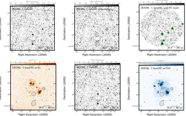
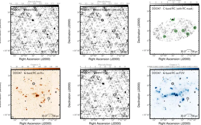
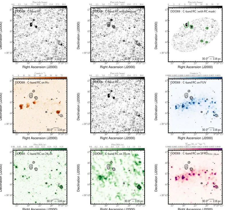
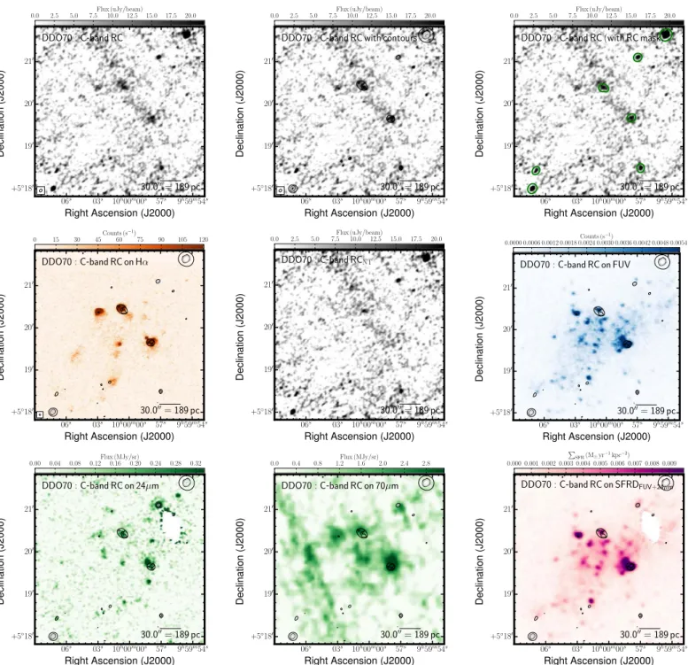
(8) The Astrophysical Journal Supplement Series, 234:29 (69pp), 2018 February. Hindson et al.. Figure 1. Multiwavelength coverage of DDO 50 displaying an 8 0×8 0 area. We show the total RC flux density at the native resolution (top left) and again with contours (top center). The lowest contour highlights low surface brightness emission at an S/N level of 3 in the image smoothed to 10″. The remaining contours are at S/N levels of 3, 6, 9, and then multiples of twice the previous contour level from our native resolution images. These contours are also superposed on ancillary LITTLE THINGS images where possible: Hα (middle left), RCNth (middle center), GALEX FUV (middle right), Spitzer24 μm (bottom left), Spitzer70 μm (bottom center), and FUV+24 μm inferred SFRD (bottom right). We also show the RC that is isolated by the RC-based and disk masking technique (top right). In this panel, the green contours outline the RC mask and includes background and ambiguous sources. The elliptical outline corresponds to the area henceforth referred to as the disk mask.. refer to these sources of RC emission as ambiguous. To illustrate our definition of ambiguous RC emission, we present four of our observations that contained such a source in Figure 2. A strong unresolved source can be seen in DDO 46 and DDO 63, while DDO 69 and IC 1613 demonstrate galaxies with significantly extended sources. Most of our observations contained at least one ambiguous source; none of these had a nonthermal luminosity that exceeded a reference threshold—that of a known bright SNR (1 × 1019 W Hz−1 or 3.3 mJy at 5 Mpc at 6 GHz). This. reference luminosity was based on observations of SNR N4449–12, which resides in the dwarf galaxy NGC 4449 at a distance of 4.2 Mpc. In 2002, this SNR had a luminosity of S6cm=4.84 mJy with a spectral index of α=−0.7 between 20 cm and 6 cm (Chomiuk & Wilcots 2009). For comparison, this is 10 times the luminosity of Cassiopeia A. Since the luminosity terminally declines for the majority of the SNR’s lifetime, we treat the observed luminosity of SNR N4449–12 in 2002 as an approximate empirical upper limit to the luminosity of an SNR. We justify our use of SNR N4449–12 8.

(9) The Astrophysical Journal Supplement Series, 234:29 (69pp), 2018 February. Hindson et al.. Figure 2. Examples of our definition of ambiguous emission (red dashed circles). We show DDO 46 and DDO 63, each of which contains an unresolved source of 1 mJy (top left) and 1.4 mJy (top right), respectively. We also show DDO 69 and IC 1613, both of which contain an extended source (bottom panels). The RC emission could not be attributed as definitely coming from a background galaxy, but at the same time was not close enough to an SF site to be confidently classified as originating from the target galaxy either; accordingly, these sources were designated ambiguous.. duration will have a slightly lower θLAS value, and for weighting schemes closer to natural weighting, the θLAS will be larger. In our observations, angular scales of ∼4 arcminutes and above may not be adequately sampled, leading to a lower than expected flux density; there are only seven galaxies with an angular size greater than 4′ (see column 4 of Table 3). Under the assumption that RC emission coincides with optical emission, it is only these galaxies that are vulnerable to having large angular structures absent in the (u, v) data. Even so, the SF in dwarf galaxies is intermittent on scales of one to a few Gyr, whereas CRe age over much shorter timescales of tens of Myr; therefore, in the majority of our sample, no significant emission is expected from, for example, a CRe halo. We note that NGC 1569 was found to have an extended radio halo extending beyond the optical emission when observed between 0.6 and 1.4 GHz (Israel & de Bruyn 1988). This is attributed to the post-starburst nature of the galaxy, which is not reflected in. as it was the most luminous from a sample of 43 SNRs from four irregular galaxies (35 of which are in galaxies that overlap with our sample, namely: NGC 1569, NGC 2366, and NGC 4214). Using the method above, we are able to classify all of the observed RC emission in our images. As an example, we show DDO 133 in Figure 3 along with the classification attributed to each source of RC emission. 3.2. Missing Large-scale Structures Owing to the way that interferometers function, large angular structures in the sky can be completely missed if their corresponding visibilities are not recorded by the interferometer. The largest angular scale (θLAS) that the VLA is sensitive to in C-configuration (shortest baseline of 35 m) at 6 cm is ∼4 arcminutes. This assumes an observation of 12 hr that is uniformly weighted and untapered. Observations of a shorter 9.

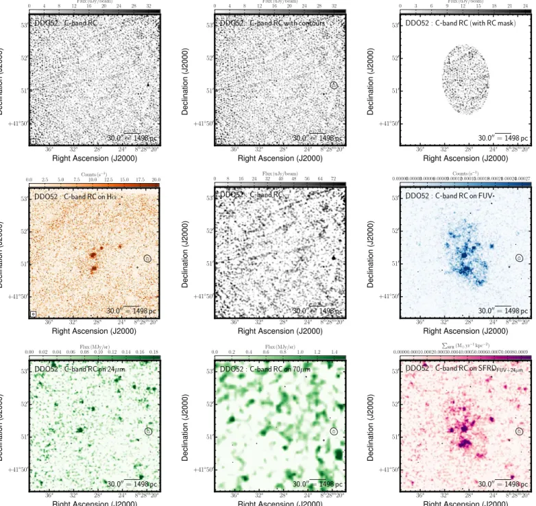
(10) The Astrophysical Journal Supplement Series, 234:29 (69pp), 2018 February. Hindson et al.. 3.4.1. Radio Continuum-based Mask. To characterize the RC emission within our images, we first estimate the spatially varying background noise across each image using the BANE algorithm (Hancock et al. 2012). BANE works by selecting each pixel in the image on a specified grid and then defines a boxed region. This region is first clipped at 3σ to remove the contribution of source pixels. The median of the remaining pixels in the box is calculated and used as the background estimate. Linear interpolation is then used to smooth the background across the image. We found that the default options for BANE, which uses a grid size of four times the beam area and a box size of five times the grid size, produced good estimates of the background noise for the majority of our images. In cases where there is large-scale extended emission such as NGC 1569 and IC 10, the grid size was increased to the approximate size of the most extended feature in the image, six and nine, respectively, and the default box size was applied. Estimating the background noise allows us to create S/N images that account for local variations in the image background caused by the primary beam sensitivity pattern and any residual low-level artifacts. This results in a robust threshold for our source detection. The average noise toward our galaxies is presented in Table 2, column 9. We apply an automated approach to source identification using the FELLWALKER source finding algorithm (Berry 2015) available in the STARLINK distribution CUPID. FELLWALKER is a thresholding approach to source detection that identifies contiguous features in an image by finding the steepest gradient for each pixel. Starting with the first pixel in an image, above a user-defined threshold, each of the surrounding pixels is inspected to locate the pixel with the highest ascending gradient; this process continues until a peak is located (i.e., a pixel surrounded by flat or descending gradients). The pixels along this path are assigned an arbitrary integer to represent their connection along a path. All pixels in the image are inspected in a similar process, and the image is segmented into clumps by grouping together all paths that lead to the same peak value. The pixels belonging to paths that lead to the same peak are then defined as belonging to that particular clump. For a full description of this process, see Berry et al. (2007). Using FELLWALKER, we create two masks for each S/N image: the first is at full resolution while the second is smoothed to an angular resolution of 10″. The former image is used to characterize unresolved point sources while the latter is used to define regions of extended emission. We assign a threshold level corresponding to an S/N level of 3 in both cases where the noise levels are derived independently for each image. Fluctuations that are smaller than the beam are excluded; they are identified as noise spikes. We verify the robustness of this approach by comparing our mask to those produced by the CLUMPFIND algorithm, which is also available in CUPID, and by checking each mask by eye to ensure that no spurious emission is included in the maps. An example of the results of this approach can be seen in the top-right panel of Figure 3 and Appendix B. Using our RC-based mask, we extract the integrated properties toward our sample of dwarf galaxies excluding background and ambiguous sources and present the results in Table 4. A table containing the integrated properties including ambiguous sources can be found in Appendix C in Table 8. In order to compare the RC emission to our ancillary data, we first investigate which masks best represent the global. Figure 3. GALEX FUV emission of DDO 133 overlaid with our RC contours. Following the procedure outlined in the text we attribute RC emission as being from either the galaxy itself (G, green), a background galaxy (B, red), or an unknown or ambiguous source (?, blue). We also overlay the optical disk size (defined by the Holmberg radius; purple dashed ellipse).. the majority of targets in our sample. We do not see any evidence of such a halo in our 6 GHz image. This may be due to spatial filtering or spectral aging, which has shifted the halo emission below our detection threshold. 3.3. Disk-integrated Quantities With background and ambiguous sources removed (see Section 3.1), emission from our RC and ancillary images was integrated within each of the dwarf galaxy’s optical disks (hereafter the disk mask; see Table 3 for the disk parameters). We also extract the integrated properties including the ambiguous sources; these can be found in Appendix C in Table 7. The semimajor axis of the disk was based on optical isophotes: using either the Holmberg radius (defined as the isophote where the B-band surface brightness drops to a magnitude of 26.66; Hunter & Elmegreen 2006) or three times the V-band disk scale length (Hunter & Elmegreen 2006) if the B-band radius was not defined. All emission outside this radius was masked. 3.4. Isolating Target RC Emission The majority of our dwarf galaxy sample only exhibits significant RC emission in isolated regions, which is attributed to both the episodic nature of SF in dwarf galaxies (e.g., Stinson et al. 2007) and the surface brightness sensitivity of our RC observations, which limits our RC maps to to detecting SFRDs greater than ∼5×10−3 Me yr−1 kpc−2. When integrated over the disk, the signal from most galaxies is dominated by the contribution of noise from the individual beams within the integration area. The uncertainty, δN, is given by srms N , where σrms is the rms noise level and N is the number of individual beams. This motivates the use of masks to isolate genuine emission from background noise (i.e., reduce the integration area, which is proportional to N) in order to improve the RC S/N. 10.

(11) The Astrophysical Journal Supplement Series, 234:29 (69pp), 2018 February. Hindson et al.. Table 3 Integrated Emission Over the Disk of the LITTLE THINGS Galaxies, Excluding Ambiguous Sources FUV. 24 μm MIR. 70 μm FIR. 6 cm RCNth. Beq. (mJy) (4). Hα (10−13 erg s−1 cm−2) (5). (mJy) (6). (10−2 Jy) (7). (10−2 Jy) (8). (mJy) (9). (μG) (10). >0.29 >0.99 >1.16 >0.61 6.70±0.60 >1.28 0.65±0.13 >0.71 >0.89 >1.48 >2.04 >0.70 >1.79 >0.57 >1.17 >1.73 >0.47 >1.19 >0.51 >0.94 >1.17 >0.87 >1.28 >0.35 2.14±0.11 0.94±0.09 4.49±0.55 96.38±0.81 >0.57 >1.28 1.01±0.14 149.60±0.31 9.66±0.59 2.62±0.48 >0.69 27.78±0.57 >2.47 0.38±0.13 1.37±0.10 >2.51. 1.95±0.03 1.28±0.03 1.08±0.02 3.00±0.03 60.10±0.49 0.29±0.01 4.32±0.04 4.39±0.04 1.66±0.01 6.27±0.04 40.44±0.10 0.68±0.01 0.82±0.01 3.66±0.08 4.55±0.03 2.21±0.02 4.85±0.05 1.53±0.01 0.80±0.01 5.91±0.03 0.57±0.01 K 0.09±0.01 K 13.02±0.45 2.41±0.03 55.81±0.87 1191.00±5.73 K K 5.38±0.09 486.70±3.02 96.38±1.11 16.26±0.17 1.48±0.02 178.60±0.92 1.28±0.01 2.75±0.04 7.48±0.15 16.81±0.06. 1.04±0.11 1.07±0.11 1.75±0.17 3.00±0.30 41.95±4.20 0.61±0.06 2.55±0.26 5.03±0.50 4.67±0.47 11.53±1.15 29.46±2.95 0.65±0.06 0.39±0.04 2.91±0.29 4.09±0.41 3.77±0.38 K K 1.05±0.11 5.55±0.56 1.15±0.12 0.80±0.08 2.00±0.20 0.10±0.01 3.02±0.32 2.84±0.29 91.86±9.24 K 0.08±0.01 0.38±0.04 2.56±0.27 746.50±75.63 37.26±3.73 11.22±1.13 2.68±0.27 80.72±8.08 4.52±0.45 K 3.67±0.38 29.53±2.96. 0.15±0.06 K K K 17.27±0.01 −0.04±0.02 2.32±0.02 1.77±0.01 −0.65±0.01 0.59±0.01 0.20±0.01 0.07±0.02 0.24±0.02 0.32±0.03 0.53±0.01 0.28±0.03 0.22±0.03 0.04±0.01 K 0.67±0.01 −0.02±0.03 −0.16±0.02 −0.12±0.01 K 5.83±0.05 0.94±0.04 6.85±0.02 3741.00±4.83 K K 0.45±0.03 705.50±13.61 65.47±0.01 11.65±0.03 0.43±0.03 199.60±0.01 K 0.37±0.03 1.87±15.06 4.61±0.01. 2.46±0.04 K K K 319.90±0.28 1.81±0.05 24.05±0.03 3.74±0.13 11.08±0.07 63.09±0.13 77.89±0.20 7.03±0.03 −0.54±0.04 14.92±0.10 33.04±0.13 3.66±0.04 16.15±0.05 10.64±0.06 K 41.94±0.10 −1.94±0.09 5.26±0.04 9.87±0.08 K 39.00±0.05 23.66±0.06 408.70±1.73 9547.00±12.08 K K 0.45±0.01 3543.00±2.66 506.20±0.30 248.10±0.41 10.20±0.11 2393.00±1.13 K 12.52±0.04 57.05±1.36 117.70±0.18. >0.29 >0.99 >1.16 >0.61 0.99±0.60 >1.28 0.24±0.13 >0.71 >0.89 >1.48 >2.04 >0.70 >1.79 >0.57 >1.17 >1.73 >0.47 >1.19 >0.51 >0.94 >1.17 >0.87 >1.28 >0.35 0.91±0.12 0.71±0.09 −0.77±0.55 −16.78±0.97 >0.57 >1.28 0.50±0.14 71.38±0.57 0.51±0.60 1.07±0.48 >0.69 10.81±0.57 >2.47 0.12±0.13 0.66±0.10 >2.51. <2 <2 <2 <2 <2 <1 <1 <1 <1 <1 <1 <2 <2 <2 <2 <1 <2 <2 <3 <1 <1 <2 <1 <3 6 5 <1 <1 <2 <2 5 17 17 17 <2 6 <1 <1 5 <1. Galaxy. Size. P.A.. 6 cm RC. (1). (′) (2). (°) (3). 1.7×1.4 1.8×1.2 3.8×3.4 4.5×2.3 7.9×5.7 2.2×1.4 2.7×1.4 4.3×4.3 4.8×2.7 7.4×4.4 6.2×5.2 2.3×1.3 2.1×1.5 3.5×1.7 4.7×3.2 3.1×1.6 1.9×1.3 4.3×2.3 1.5×1.0 4.6×2.9 2.1×1.7 2.6×1.3 8.0×3.6 1.3×1.0 1.7×1.0 1.5×1.2 18.2×14.7 11.6×9.1 1.9×1.0 1.5×1.1 2.0×0.9 2.3×1.3 9.4×4.0 4.8×4.8 2.9×1.9 9.3×8.5 4.3×2.3 2.5×1.4 2.2×1.1 11.6×5.1. 80 6 84 −79 18 4 81 0 −64 88 42 76 −69 −41 −6 46 51 89 −24 −25 37 −85 −58 7 85 90 71 −38 −3 86 −51 −59 33 0 18 16 88 −60 −11 −2. CVn I dwA DDO 43 DDO 46V DDO 47 DDO 50 DDO 52 DDO 53 DDO 63 DDO 69 DDO 70 DDO 75 DDO 87 DDO 101 DDO 126 DDO 133 DDO 154 DDO 155 DDO 165 DDO 167 DDO 168 DDO 187 DDO 210 DDO 216 F564-V03V Haro 29 Haro 36V IC 1613 IC 10V LGS 3 M81 dwAV Mrk 178 NGC 1569V NGC 2366 NGC 3738 NGC 4163 NGC 4214 Sag DIGV UGC 8508 VIIZw 403 WLM. Note. (Column 1) Name of dwarf galaxy. The superscript “V” means that disk properties (columns 2–5) are taken from V-band data; for all others, properties are taken from the B-band; (Columns 2 and 3) Size (major and minor axes) and position angle (P.A.) of the optical disk (Hunter & Elmegreen 2006); (Column 4) 6 cm (∼6 GHz) radio continuum flux density. This value and those following have ambiguous sources removed. For values where we retain ambiguous sources, see Appendix C; (Column 5) Hα flux; (Column 6) GALEX FUV flux density; (Column 7) Spitzer24 μm MIR flux density; (Column 8) Spitzer70 μm FIR flux density; (Column 9) 6 cm (∼6 GHz) radio continuum nonthermal (synchrotron) flux density. All RCNth emission is assumed to be synchrotron and is inferred by subtracting the RCTh component from the total RC following Deeg et al. (1997). The quantity in parentheses is the amount that was regarded as ambiguous. (Column 10) Equipartition magnetic field strength in the plane of the sky (see Equation(3) in Beck & Krause 2005).. emission in our dwarf galaxies. Ideally, we would like to compare the various quantities over the same optically derived disk mask since our ancillary data is general present emission over a large fraction of the disk. However, if we integrate the RC emission over the disk, we find that only 11 of our 40 observations have significant integrated RC flux density measurements. Using instead our RC mask, we identify RC emission associated with 22 of the 40 LITTLE THINGS galaxies (excluding ambiguous sources); eight are new RC detections. It is for this reason that in the course of the analysis. of our data we will present results integrated over both the RCand disk-based masks. 3.5. Radio Continuum Source Counts To test the robustness of our source identification and extraction approach, we determine the radio continuum source counts from our images. We compare these to Huynh et al. (2012), who performed 5.5 GHz observations with the Australia Telescope Compact Array of a 900 arcmin2 region with a restoring beam of 4 9×2 0 and an rms noise of. 11.

(12) (1). R.A hh mm ss.s (2). Decl. dd mm ss.s (3). fdisk (%) (4). 6 cm RC (mJy) (5). Hα (10−13 erg s−1 cm−2) (6). FUV (mJy) (7). 24 μm MIR (10−2 Jy) (8). 70 μm FIR (10−2 Jy) (9). 6 cm RCNth (mJy) (10). Beq (μG) (11). DDO 46 DDO 47 DDO 50 DDO 53 DDO 63 DDO 70 DDO 75 DDO 126 DDO 155 DDO 168 Haro 29 Haro 36 IC 1613 IC 10 Mrk 178 NGC 1569 NGC 2366 NGC 3738 NGC 4214 UGC 8508 VIIZw 403 WLM. 07 41 26.6 07 41 55.3 08 19 08.7 08 34 08.0 09 40 30.4 10 00 00.9 10 10 59.2 12 27 06.5 12 58 39.8 13 14 27.2 12 26 16.7 12 46 56.3 01 04 49.2 00 20 17.5 11 33 29.0 04 30 49.8 07 28 48.8 11 35 49.0 12 15 39.2 13 30 44.9 11 27 58.2 00 01 59.2. +40 06 39 +16 48 08 +70 43 25 +66 10 37 +71 11 02 +05 19 50 −04 41 56 +37 08 23 +14 13 10 +45 55 46 +48 29 38 +51 36 48 +02 07 48 +59 18 14 +49 14 24 +64 50 51 +69 12 22 +54 31 23 +36 19 38 +54 54 29 +78 59 39 −15 27 41. 0.1 0.1 2.2 3.2 0.1 0.1 0.3 2.3 5.2 0.2 13.4 9.3 0.7 22.9 3.8 126.3 2.2 6.2 2.2 3.2 15.8 0.1. 0.02±0.01 0.03±0.01 6.27±0.09 0.33±0.02 0.06±0.01 0.07±0.02 0.24±0.03 0.35±0.03 0.28±0.04 0.11±0.01 2.01±0.04 0.37±0.03 2.51±0.05 99.33±0.39 0.46±0.03 155.40±0.34 11.98±0.09 2.98±0.12 22.58±0.08 0.16±0.02 1.29±0.04 0.16±0.02. 0.16±0.01 0.15±0.01 25.28±0.42 1.90±0.04 0.24±0.01 0.29±0.02 2.87±0.06 1.46±0.07 2.23±0.04 0.24±0.01 12.54±0.45 1.17±0.03 10.26±0.43 887.90±5.68 2.33±0.08 503.90±3.03 66.97±1.10 11.83±0.17 117.20±0.91 0.65±0.02 6.49±0.15 0.79±0.05. 0.02±0.01 0.05±0.01 7.45±0.76 0.71±0.07 0.14±0.02 0.21±0.03 0.85±0.09 0.54±0.06 K 0.12±0.01 2.65±0.29 1.94±0.21 5.08±0.71 K 0.97±0.12 755.60±76.53 12.64±1.28 7.29±0.75 32.63±3.29 K 3.21±0.33 0.10±0.01. K K 7.69±0.06 1.32±0.09 0.04±0.34 0.03±0.34 0.07±0.23 0.15±0.20 0.15±0.12 0.04±0.18 4.96±0.14 0.41±0.13 1.69±0.23 1369.00±10.10 0.16±0.17 716.20±12.11 52.01±0.04 7.58±0.13 140.40±0.09 0.06±0.15 2.10±37.85 0.27±0.30. K K 53.17±0.04 5.30±0.01 0.33±0.01 0.34±0.01 1.61±0.01 2.11±0.02 2.42±0.01 0.67±0.01 21.21±0.02 6.88±0.02 23.10±0.12 5482.00±6.68 0.16±0.01 3758.00±2.99 179.50±0.05 91.12±0.10 941.10±0.17 1.18±0.01 33.77±0.54 0.31±0.01. 0.01±0.01 0.02±0.01 3.95±0.10 0.16±0.02 0.04±0.01 0.04±0.02 0.01±0.01 0.23±0.03 0.08±0.04 0.09±0.01 0.82±0.06 0.26±0.03 1.63±0.06 14.96±0.66 0.25±0.03 74.41±0.60 5.65±0.14 1.85±0.12 11.55±0.12 0.10±0.02 0.68±0.04 0.01±0.01. <1 <1 4 4 2 <1 <1 3 <1 2 6 4 3 8 4 17 5 7 6 2 5 <1. Galaxy. 12. The Astrophysical Journal Supplement Series, 234:29 (69pp), 2018 February. Table 4 Integrated Emission Over the RC Mask of the LITTLE THINGS Galaxies, Excluding Ambiguous Sources. Note. (Column 1) Name of dwarf galaxy; (Columns 2 and 3) Equatorial coordinates (J2000) of center of the galaxy defined by the optical disk; (Column 4) Fraction of the disk (see Table 3) that has significant RC emission; (Column 5) 6 cm (∼6 GHz) radio continuum flux density. This value and those following have ambiguous sources removed. For values where we retain ambiguous sources, see Appendix C; (Column 6) Hα flux; (Column 7) GALEX FUV flux density; (Column 8) Spitzer24 μm MIR flux density; (Column 9) Spitzer70 μm FIR flux density; (Column 10) 6 cm (∼6 GHz) radio continuum nonthermal (synchrotron) flux density. All RCNth emission is assumed to be synchrotron and is inferred by subtracting the RCTh component from the total RC following Deeg et al. (1997). The quantity in parentheses is the amount that was regarded as ambiguous. (Column 11) Equipartition magnetic field strength in the plane of the sky (see Equation(3) in Beck & Krause 2005).. Hindson et al..

(13) The Astrophysical Journal Supplement Series, 234:29 (69pp), 2018 February. Hindson et al.. Table 5 6 cm Source Counts N. ΔS (μJy) 46–73 73–116 116–183 183–290 290–460 460–728 728–1155 1155–1831 1831–2901 2901–4598 4598–11478 11478–28653. dNc/dS. Nc. (sr all. bg. amb. all. bg. amb. all. 60 52 55 25 24 26 10 13 6 7 9 11. 50 40 37 15 15 17 3 3 1 0 1 0. 52 42 43 18 16 17 5 5 1 1 1 0. 180.18 125.43 124.68 55.52 52.78 56.74 21.65 27.96 12.86 14.90 18.98 23.03. 150.15 96.48 83.87 33.31 32.99 37.10 6.50 6.45 2.14 0.00 2.11 0.00. 156.15 101.31 97.47 39.98 35.19 37.10 10.83 10.75 2.14 2.13 2.11 0.00. 1983.58 785.19 485.42 132.29 78.56 55.06 12.93 10.68 3.74 2.53 1.29 0.63. −1. Nc/Nexp. −1. Jy ) bg. 1652.99 603.99 326.55 79.37 49.10 36.00 3.88 2.47 0.62 0.00 0.14 0.00. amb. all. bg. amb. 1719.11 634.19 379.51 95.25 52.37 36.00 6.47 4.11 0.62 0.36 0.14 0.00. 0.44±0.03 0.60±0.05 1.23±0.11 1.08±0.15 2.04±0.28 4.39±0.58 3.34±0.72 8.61±1.63 7.91±2.20 18.27±4.73 31.03±7.12 148.48±30.94. 0.37±0.03 0.46±0.05 0.83±0.09 0.65±0.11 1.27±0.22 2.87±0.47 1.00±0.39 1.99±0.78 1.32±0.90 0.00±0.00 3.45±2.37 0.00±0.00. 0.38±0.03 0.49±0.05 0.96±0.10 0.78±0.12 1.36±0.23 2.87±0.47 1.67±0.51 3.31±1.01 1.32±0.90 2.61±1.79 3.45±2.37 0.00±0.00. Note. 6 cm (6.2 GHz) source counts. (Column 1) flux density bins taken from Huynh et al. (2012) converted to 6.2 GHz assuming a spectral index of −0.7; (Column 2) number of >5σrms RC source counts. We count all sources in the images (all), sources identified as background (bg), and sources identified as background or ambiguous (amb). (Column 3) the completeness and resolution-corrected RC source counts. (Column 4) the corrected RC source count rate—the number of sources found per steradian normalized to the midpoint of the flux density bin. (Column 5) corrected source counts normalized by the expected number from a non-evolving Euclidean model.. 12 μJy beam−1. After correcting for incompleteness and resolution bias, they present normalized source counts in 10 flux density bins ranging between 50 and 5000 μJy (see their Table 2). Our images were generated using a restoring beam of approximately 3″ and attained an rms noise of ∼6 μJy beam−1. Therefore, the sensitivity per beam in our data is comparable to that from Huynh et al. (2012). We scale the Huynh et al. (2012) bins to 6.2 GHz, the effective frequency for most of our images, assuming a spectral index of −0.7±0.2. This assumption is supported by various studies that show that the average spectral index of star-forming galaxies is narrowly concentrated around ∼−0.7 with a small dispersion of 0.2 (Condon 1992; Niklas et al. 1997; Lisenfeld & Volk 2000). For each bin, we cycled through our images, counting all sources with flux densities in the range ΔS. We count sources only from within a 4′ circular aperture centered on the image pointing reference to avoid regions where the primary beam response leads to higher noise levels. Sources are assigned to three different groups following our source classification approach described in Section 3.1. The first group includes all sources in the field including the galaxy emission, the second counts only sources we are confident are background sources, and the final group consists of both background and ambiguous sources. Sources were not counted if, in the given bin, the low end of the bin was less than five times the rms noise from the image (this only affected the two lowest bins because of a few high rms images). No attempt was made to count resolved sources originating from the same source (e.g., radio lobes, multiple SF regions from a dwarf, etc.). To estimate the completeness of our source catalog, we follow a similar approach to Huynh et al. (2012) and perform a Monte Carlo simulation. We inject a synthetic Gaussian source with a randomly generated position and brightness from 30 to 3000 μJy into our image and then apply the FELLWALKER source detection algorithm following the same approach as described in Section 3.4 to see if the source is recovered. We do. this 8000 times and find that sources with flux densities of 5σrms (∼50 μJy) have a detection rate of 50%, where σrms is the rms noise in the image. The detection rate rises steeply to 90% at 120 μJy. We also correct for the resolution bias following the same approach as Huynh et al. (2012). This correction accounts for sources with weak extended emission and large total integrated flux densities that have peaks that fall below the detection threshold. Given our slightly higher sensitivity and resolution ,we find lower resolution correction factors than Huynh et al. (2012), with values of 1.24 in our lowest bin and 1.03 in our highest bin. We present the results of our source counts in Table 5. For each bin, we present the raw source counts (N) and the counts corrected for completeness and resolution bias (Nc). We determine the RC source count rate (dNc/dS), which corresponds to the number of sources found per steradian normalized to the midpoint of the flux bin. Finally, we normalize our corrected source counts by dividing by the expected number of sources (Nexp) derived from a nonevolving Euclidean model using the relation N (>S6 cm ) = 1.5 60 * S6-cm . The Poissonian errors are presented for the normalized and corrected counts with the resolution and completeness correction uncertainties (10% and 2%–5%, respectively) added in quadrature. In Figure 4, we present a comparison of our source counts using all sources (black squares), only background sources (blue triangles), and both background and ambiguous sources (green pentagons). We compare our results to the corrected and normalized source counts of Huynh et al. (2012; red circles). This plot clearly shows that our counts are consistent with those of Huynh et al. (2012) until ∼103 μJy. Beyond this flux, we see that including galaxy emission in our source counts leads to higher counts than those found in Huynh et al. (2012), particularly at flux densities above 8.6 mJy. Ideally, we would like to use the source counts to test the reliability of our source identification approach. In particular, we would like to test whether sources we define as ambiguous are background 13.