Balance of payments liberalization: effects on growth, employment and income in Argentina

Texto completo

(1)CEPA Center for Economic Policy Analysis. Balance-of-payments Liberalization: Effects on Growth, Employment and Income in Argentina Roberto Frenkel and Martín González Rozada (Centro de Estudios de Estado y Sociedad, Buenos Aires). CEPA Working Paper Series I Globalization, Labor Markets, and Social Policy A Project Funded by the John D. and Catherine T. MacArthur Foundation Working Paper No. 13 February 2000. Center for Economic Policy Analysis New School University 80 Fifth Avenue, Fifth Floor, New York, NY 10011-8002 Tel. 212.229.5901 Fax 212.229.5903 www.newschool.edu/cepa.

(2) Balance-of-payments liberalization. Effects on growth, employment and income in Argentina Roberto Frenkel* Martín González Rozada*. CEDES Buenos Aires, July 1999. *CEDES. The authors thank Carola Ramón for her collaboration and Lance Taylor for his comments on the draft. The authors also wish to thank the participants in the New York, Rio de Janeiro and San Salvador seminars for their comments on the draft..

(3) 2. Introduction. In the first half of the nineties, Argentina witnessed an impressive process of market-friendly reforms, targeting the privatization of a large proportion of state-owned enterprises, as well as both trade and financial opening. At the same time the country was emerging from a period of extreme instability in prices which had led to two brief hyperinflationary episodes in 1989 and 1990. This price stabilization was concurrent with a strong recovery in growth that had its dark side: unemployment grew significantly and inequality deepened. One of the main structural reforms in the nineties was the opening of the economy to international trade. It was already in 1988 that notable inroads had been made in this direction. However, in the nineties the previous gradual approach was abandoned and the opening was accelerated.. Average import tariffs were reduced from 26.5 percent in. October 1989 to 9.7 percent in April 1991. In addition, specific duties were eliminated, as were quantitative restrictions on imports.1 Privatizations, for their part, commenced in 1990 with the transfer of the telephone company and the national airlines. By late 1994 the major part of the state-owned firms producing goods and services had been sold, including the most important ones: the oil company (YPF) and the producers and distributors of electric power. This process covered a wide range of productive areas from iron and steel works to petrochemicals and gas. In some cases (oil fields, railways, ports, highways, waterworks and sewage, and television channels and radio stations) the government resorted to concession mechanisms. Several legal norms marked the structural reform process. First was the Law of the State Reform (August 1989) which established the legal bases for the privatization of stateowned enterprises with the capitalization of public debt. Second, in order to improve the performance of the public accounts, the Law of Economic Emergency (September 1989) 1. Between 1987 and 1988 the average tariff dropped from 43 percent to 30 percent and quantitative restrictions were reduced. In October 1989, some 807 tariff lines were subject to "transitory additional duties," 122 to import licensing and 129 to specific duties. In April 1991 not one tariff line was subject to either specific duties, transitory additional duties or to import licenses. Restrictions remained in effect for only 25 tariff itemsthose corresponding to motor vehicles and auto partsout of a total of 10,000. Special rates were also maintained for motor vehicles and electronics, which were subject to a 35 percent tariff. The tariff structure in April 1991 included three rates: zero for raw material, 11 percent for inputs and capital.

(4) 3. suspended several subsidy mechanisms, such as those that were implicit in the industrial and regional promotion regimes. This law established equal treatment for foreign and domestic capital invested in productive activities in the country. In this way, prior approval for direct foreign investment was no longer necessary. In addition, in November 1991, a Deregulation Decree eliminated a wide set of regulations encompassing diverse economic activities. The most important legal instrument of the stabilization process was the Convertibility Law (March 1991) that established a fixed peso-dollar parity and validated contracts in any foreign currency. It also stipulated that the Central Bank must back 100 percent of its monetary base with foreign reserves.. The new Central Bank Charter. (September 1992) suppressed the official guarantee on deposits and fixed narrow limits whereby it could purchase public bonds and lend to commercial banks. The law also established the autonomy of the Central Bank. In practice, the Convertibility Law transformed the Central Bank into a currency board and completed the deregulation of the capital account of the balance of payments. So that from early 1991, both trade and capital flows were fully liberalized. This research paper gives a summary2 analysis of the growth process, the performance of the labor market and the evolution of income and wages in the context generated by the structural reforms, as well as a discussion of the stabilization policies that were applied in the nineties.. There are seven sections to the paper, following the. introduction. Section I presents some aspects of the macroeconomic dynamics, mainly in the form of graphs that facilitate the comparison between the eighties and the nineties and highlight the stylized facts of the latter. In this shorter version we have solely presented the most relevant features for the analysis of income and employment.. Section II presents an. econometric model that describes the macroeconomic performance in the nineties and summarizes the estimation results. Section III focuses on the behavior of the urban labor market at the national level and in Greater Buenos Aires (GBA).. The presentation. compares the eighties with the nineties and stresses the main stylized features of the latter. goods, and 22 percent for final goods. See Damill and Keifman (1993). Since 1995 the Argentine tariff structure has been that of the MERCOSUR (with some exceptions). 2 See Frenkel and González Rozada (1999a) for the complete version of the report..

(5) 4. Section IV includes the formulation and estimation of an econometric model of the aggregate urban labor market. In Section V GBA data are utilized to analyze variations in urban employment by sector of activity and socio-demographic characteristics.. The. manufacturing sector is by far the most important urban tradable activity. The analysis shows that the contraction in employment in this sector explains two-thirds of the fall in total full-time employment observed in the nineties. Section VI studies the performance of production, employment and productivity in the manufacturing sector using data from the industrial survey. An econometric model of labor demand in this sector is presented. The econometric estimations, together with the trade information on the manufacturing sector, are utilized to separate and calculate the different effects on the employment contraction in this sector. Finally, Section VII focuses on income and its distribution..

(6) 5. I. Stylized features of the macroeconomic dynamics.3. The short-run cycle and growth. Graph 1 shows the evolution of quarterly GDP (in logs) in both the eighties and nineties. The trend is obtained using the Hodrick-Prescott filter (with the conventional parameter). As can be seen, GDP in the eighties fluctuated cyclically on a stagnant trend while showing a clearly positive trend in the nineties. The HP filter in the graph indicates a new growth trend in the nineties, with an annual rate of 4.8 percent. There is a first expansionary phase that lasted until 1994. This expansion begins before the Convertibility Plan was launched, in the second semester of 1990, and reached its peak in the second semester of 1994.4 Between the second semester in 1990 and that of 1994 seasonally adjusted GDP grew by 35.7 percent (an average annual rate of 8%). The second phase marks a recession associated with the tequila effect in 1995, which produced a 6.8 percent contraction in GDP between the second semesters in 1994 and 1995. Recovery from the recession began in the second semester in 1996, with an activity level return to a level similar to that of the second semester of 1994. Finally, in late 1996, the country enters its most recent expansionary phase, with growth accelerating as a result of the large capital inflows. Between the second semesters of 1996 and 1997, GDP increased by 9.2 percent. However, the expansion decelerated after October 1997, following the Asian crisis. GDP has exhibited a recessionary trend since the second semester of 1998.. Foreign trade and the balance of payments. During the first expansionary phase, the export ratio at constant prices (Graph 2) remained practically stagnant. This ratio jumps between 1994 and 1995 but later shows a stagnant trend. On the other hand, the import ratio at constant prices sharply increases. 3. Sections I and II are based on research carried out together with Mario Damill. More detailed analysis can be seen in Fanelli and Frenkel (1999) and in Frenkel, Fanelli and Bonvecchi (1998). 4 As data on employment are available only by semester, it is useful for the sake of the analysis to present GDP evolution in the same way..

(7) 6. during the first expansionary phase, then decreases with the recession, only to steadily increase during the second expansion. On observing trends in the foreign account at current prices, the dynamics of the balance of payments appears halted with the 1995 crisis (Graphs 3 and 4). During the first phase, capital inflows grow annually until 1993 and then show a decline in 1994, when the United States interest rates are raised. The country risk rate descends until 1993, then rises in 1994 (Graph 7). On the other hand, the current account deficit exhibits a growing trend in the first expansionary phase, and given that before 1994 capital inflows were mainly private and systematically larger than the current account deficit, reserves increase (Graphs 5 and 6). With the decline in private capital inflows in 1994, reserves tend to stagnate. This change in the trend was followed in the first quarter of 1995 by abrupt capital outflows and a contraction in reserves caused by the tequila crisis. Following this crisis, there is a transition phase in the evolution of the balance of payments that extends to the third quarter of 1996. This is characterized, in the first place, by a transitory reduction in the current account deficit explained by the behavior of the trade balance. The above jump in export volume is mainly compounded by the impact of Brazil's Real Plan on Argentina and increasing prices in agricultural and oil commodities. On the other hand, the level of imports dropped as a result of the recession. Altogether, these effects made it possible to achieve a transitory trade balance. During this phase capital inflows correspond exclusively to the public sector, thanks to the rescue operation led by the IMF. From late 1996 the evolution of the balance of payments once more shows similar features to that of the first expansionary phase of 1991-93. This recent expansionary phase extends from late 1996 to the Asian crisis. Net capital inflows, again mostly private, are similar to the maximum annual inflow registered before 1994. The current account deficit tends to increase swiftly, mainly because of the rise in imports. However, just as in the first expansionary phase, capital inflows surpass the deficit and reserves accumulate. The country-risk rate tends to fall after 1995 and reaches a minimum (similar to that of 1993) in the months preceding the Asian crisis. The deceleration in growth in late 1997 and the new recessionary phase in 1998, are associated with successive higher country-risk rates and lower private capital flows..

(8) 7. Sources of demand expansion, savings and investment During the first expansionary phase not only consumption but also investment5 contribute to the expansion in domestic absorption. The investment rate at the end of the eighties was at its lowest point ever and tended to increase rapidly in this first phase, thanks to the exchange rate appreciation which raised the purchasing power of (imported) capital goods for a determined savings rate.. With the 1995 crisis the proportions of both. consumption and investment were reduced.. After the crisis, from 1996 on, both. components of the absorption increased their participation in the product. Although the consumption rate remained lower than those in the first expansionary phase, the investment rate continued to climb. Until 1994, in the first expansionary phase, consumption dominates aggregate demand increases, particularly in the first two years, and there is no export growth contribution. During the 1995 crisis, contractions in consumption and investment equally contribute to the fall in aggregate demand, while, for just this time, the increase in exports plays a significant counter-cyclical role. The recovery from the post-tequila phase was again steered by consumption, but the contributions of investment and consumption tend to converge in 1997 when growth accelerated. The savings rate in the nineties falls systematically below that of the eighties. The difference with the investment rate tends to widen in the first expansionary phase despite the tendency of the savings rate to rise in the second half of the phases. The rates converge in the 1995 crisis owing to the sharp reduction in investment, together with a fall in the savings rate. The adjustment mechanism was the contraction of the product along with a mainly exogenous increase in exports. The savings-investment gap tends to widen again in the post-tequila phase, reaching its 1994 level in 1997.. 5. Argentina's National Accounts system does not have an independent consumption estimate. The variable is a residual calculation based on the estimations of the other components of the Accounts. The estimated consumption thus includes inventory variations. The investment variable is the gross fixed investment..

(9) 8. Inflation. The consumer price dynamics (a proxy for non-tradable goods) is most commonly observed in shock stabilization plans with an exchange-rate anchor (Graph 8). The "inertial inflation" persists for some time via the survival of price and wage indexation mechanisms. Given that inflation is gradually reduced in a context of strong money, credit and demand expansion, the process can only be attributed to the stabilizing role of the fixed exchange rate in a context of greater trade opening. Once the exchange rate is fixed, the inflation rate of consumer prices gradually converged with the international inflation rate. This process took approximately three years. In contrast, the appreciation of the exchange rate in the previous year contributed to the immediate convergence of tradable goods prices (approximated by the wholesale price index). In this way, international prices operated as a constraint on domestic tradable ones from the very moment the plan was launched.. Relative prices. Relative prices in the nineties differ greatly from those that characterized the previous decade.. Trade and financial opening affected macroeconomic behavior and. employment mainly via changes in relative prices. Assuming the launch of the Convertibility Plan as the starting point of the new regime, the major part of the change takes place within relatively few months before and after the launch. The change in relative prices takes the form of a shock, so relative prices are determined from the very beginning. The changes that are produced from 1991 are of secondary importance to those that occurred upon the launch. These considerations are clearly valid for the real exchange rate and wages valued at constant dollars6 (Graphs 9 and 10). The following table shows the average values for the different periods.. 6. The wage considered here is the industrial manufacturing wage published by FIEL, corresponding to a sample of large-sized firms. The dynamic in the nineties differs from that of the wage in INDEC's household survey, but this difference does not affect the point referring to the change between the eighties and the nineties..

(10) 9. 1986-90. 1986-88 1990:4-1991:1 1991:2-1998 1994-98. Real exchange rate. 1.22. 1.16. 0.62. 0.50. 0.49.. Wages in const. dollars.. 0.76. 0.83. 1.33. 1.48. 1.51. As can be seen, the changes in relative prices domestic producers of tradable goods faced were in full effect from the beginning of the period. The relative prices characterizing the period were determined as a shock from the first moment. Thus, it is reasonable to consider the transformations observed in the productive structure and in the technology and organization of the firms as adaptation processes to these new conditions rather than as gradual changes based on the gradual changes in relative prices. Taking into account the behavior of inflation and relative prices and the focus of the paper, we can dichotomize without significant loss the analysis of prices and quantities and consider prices as exogenous in the macroeconomic model below.. II. The macroeconomic model. This section presents a simple model of the macroeconomic performance under the convertibility regime. The model ignores sustainability conditions and external and/or financial crises in order to focus exclusively on the economy's short-run real dynamics and growth. Capital flows, the country risk premium and exports are exogenous. The exogenous character of the capital flows and the country risk premium is a simplification intended to stress that both variables have been essentially determined by international conditions. The model determines the evolution of the balance of payments, the product, investment and employment.7 This section does not include the equations for the labor market. These will be presented later..

(11) 10. Definitions and equations. R = X - M + Z + CK,. where dR is the international reserves variation of the banking. system (including the foreign currency denominated segment); X: exports; M: imports; Z: foreign factors service payments; CK: the capital account balance. CC = X - M + Z is the current account balance. dB = dR . TC. is the currency board rule. The monetary base variation equals reserves. variation times the exchange rate. BR = B / P is the real value of the monetary base. P is the local price level (CPI). TCR = TC . P* / P. is the real exchange rate. TC = 1 (Convertibility Law). P* is the USA. price level (CPI). r = r* + PRISK.. The relevant interest rate equals the international rate plus the country. risk premium. Y = Y (BR , r ) YBR > 0; Yr < 0, where Y is the GDP8. M = M (Y , TCR) MY > 0; MTCR < 0. I = I (Y , r) IY > 0; Ir < 0, where I is investment. PRISK = PRISK ( θ , CC ). PRISKCC < 0 and so rM > 0. θ is an exogenous vector. representing the international financial markets conditions.9 Z = - r* ∫ CK(h) dh. where ∫ CK(h) dh is the accumulated stock of net capital flows. between time 0 and time t.. As a short run dynamic model, the reduced equations express the activity level, investment and imports as functions of exports, capital flows and the country risk premium. The long-run dynamics implied by the model can be illustrated by the following exercise. Suppose there are balance-of-payments surplus initial conditions, exports grow on a linear trend, the international interest rate and the country risk premium are constant and there is a constant positive capital inflow. With these simplifying assumptions the model can be easily resolved in a differential equation in the reserves variation. This 7. As the National Accounts system has no independent estimation of consumption, the model includes an aggregate product equation and an investment equation. 8 Si X = X(Z, Y, ...) ; XZ = dX/dZ , XY = dX/dY , etc..

(12) 11. equation tells us that pushed by the capital inflows the economy is initially growing and accumulating reserves. The expansion induces increasing imports. The external debt interest payments and the foreign capital services also have growing trends, as the capital inflows accumulate in a growing stock of foreign liabilities. The current account deficit rises and the initial balance of payments surplus tends to fall, reducing the reserves and the economy rates of growth. The reserves, the monetary base and the GDP tend to linear trends. The slopes of those trends are positive or negative depending exclusively on the difference between the trend in exports and the trend in foreign factors payments (X - r* CK). This means that in a context of constant capital inflows the economy experiences an initial boom and a decelerating growth trend tending to a long term path which slope, positive or negative, depends exclusively on the rate of growth of exports.. The econometric estimations Our econometric estimations of the model equations show10 that the evolution of the balance of payments and the relevant interest rate tells quite accurately the convertibility period macroeconomic history. The balance of payments evolution strongly depends on capital inflows. The capital account variance explains 36 percent of the reserves variation variance. The one quarter lagged reserves rate explains 42 percent of the quarterly GDP rate. On the other hand, GDP and investment show a highly significant direct link with the international financial conditions confronted by the country. The relevant interest rate variance explains 40 percent of the GDP quarterly rate of growth variance. Quantity (capital inflows) and price (relevant interest rate) factors, mainly determined by the volatile international financial context, explain in a great deal the ups and downs of activity level and investment. globalization.. This is not an extraordinary characteristic in times of financial. Argentina's distinctive characteristic is the close connection with the. international financial markets established by the Convertibility regime. 9. The sensitivity of the country risk premimum to the current account balance only affects the speed of adjustment of GDP to the balance of payment variations. 10 We estimated the product equation in quarterly rates of growth and in deviations with respect to the log trend. The imports and investment equations were estimated in quarterly rates of growth. All by OLS with heteroskedasticity consistent variances estimators. In all cases we obtained significant (5%) coefficients estimators and satisfactory usual fit tests. The estimations can be seen in the complete version of the paper..

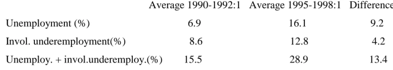
(13) 12. III. The evolution of national urban employment. Graph 11 shows the evolution of the activity rates (NTPEAPOB), employment (NTASAN) and full-time employment11 (NTASANPLE) from 1980 as proportions of the urban population. The graph also presents trends obtained using the Hodrick-Prescott filter. The trend in the activity rate is upward sloping from the mid-eighties. The long-run trend estimated with the HP filter from the second half of the eighties is an annual 0.9 percent. Nevertheless, as can be seen in the graph, the nineties starts with an activity rate that falls below the long-run trend. The trend estimated on the series from the second semester of 1990 is slightly higher than one percent per year. In the nineties the negative trend in full-time employment accentuates and the total employment trend turns negative, although the latter is cushioned by the rise in involuntary underemployment. The full-time employment curve in the nineties shows a cycle with a peak in the second semester of 1992. From then until the second semester of 1996, fulltime employment shows a steady decline, more so in the first semester of 1995 due to the recession resulting from the tequila effect. A recovery in the full-time employment rate can be observed in 1997, associated with the strong expansion mentioned above. The areas between the activity and employment curves and between the total and full-time employment curves in Graph 11 are the unemployment rate (NTUNEMP) and the involuntary underemployment rate (NTASANSUB), respectively, as proportions of the urban population. The trends in the nineties and the importance the contraction in full-time employment had in explaining the rise in both unemployment and involuntary underemployment are highlighted. The variation in these rates in the nineties, measured as percentages of the active population, are summarized in the following table:. 11. Full-time employment includes those persons working 35 or more hours per week and those choosing to work less than 35 hours. Data utilized correspond to urban conglomerates covered by INDEC's Household Survey. These surveys are carried out twice a year in April and October. As these months are central to the first and second semester of the year, we present the analysis by semester..

(14) 13. Average 1990-1992:1 Average 1995-1998:1 Difference Unemployment (%). 6.9. 16.1. 9.2. Invol. underemployment(%). 8.6. 12.8. 4.2. 15.5. 28.9. 13.4. Unemploy. + invol.underemploy.(%). The contraction in full-time employment is the crucial variable in explaining the increase in unemployment and involuntary underemployment.. Graph 12 shows the. relationship between the full-time employment rate (as a proportion of the urban population) and the GDP, as an index with base = 1 in the second semester of 1990. As can be seen, in the eighties and until the second semester of 1990 the full-time employment rate and the product evolve on the same trend. However, these trends have opposite signs in the nineties.. Data from Greater Buenos Aires. Figure 1 presents four tables on Greater Buenos Aires in the nineties. The tables show the employment rate, the full-time employment rate (35 hours and over), the involuntary underemployment rate (TASANSUBI) and the voluntary underemployment rate (TASANSUBV), as proportions of the GBA population12. The employment rate of the first graph is the sum of the three other components. Two features stand out regarding the behavior of these variables.. First of all, full-time employment and voluntary. underemployment vary jointly in a cycle that hits a maximum around the first semester of 1992 and a minimum in the second semester of 1996.. Second, involuntary. underemployment varies counter-cyclically, reaching a minimum around the second semester of 1992 and a maximum in the second semester of 1996. The dynamics of involuntary underemployment is analogous to the dynamics of unemployment. These observations suggest aggregating full-time employment and voluntary underemployment as. 12. The activity and employment levels in GBA are higher than those at the national level, but the dynamic and the changes between the eighties and the nineties are similar and we will therefore not comment on them. In the cases of equivalent series the name of the series is maintained without the initial letter N (e.g., TPEAPOB is the activity rate in GBA, equivalent to NTPEAPOB at the national level)..

(15) 14. the. dependent. variable. in. the. employment. model. and. treating. involuntary. underemployment as a type of unemployment.. IV. The aggregate model of the labor market. From the preceding section it can clearly be seen that a structural change in labor demand occurred in the nineties.. The new incentives and constraints induced a. restructuring in foreign trade and domestic production, the organization and technology of production and labor demand. Let us assume that the macroeconomic dynamics analyzed in Section I affected the firms via changes in domestic demand and relative prices.13 The incentives and constraints that characterized the nineties did not arise gradually. The relative prices in effect during the period had been defined practically from the very beginning as we explained in Section I. In contrast, the restructuring of labor demand induced by the new incentives and constraints as a gradually developing process throughout the nineties can be considered. The formal treatment we give this issue follows. We assume a labor demand equation of the form log E = α log Y + γ log (W / PK) + δ where E is employment, Y the product and W/PK the wage/capital goods relative price. Say t = 0 is a point in time before the changes, i.e. the eighties, and t = 1 is a point in time when the process of changes in the labor demand developed considerably, i.e. 1996. Thus: log E0 = α log Y0 + γ log (W0 / PK0) + δ0. and. log E1 = α log Y1 + γ log (W1 / PK1) + δ1 The difference between both observations being: ∆ log E = α ∆ log Y + (B1 - B0) with B0 = γ log (W0 / PK0) + δ0 and B1 = γ log (W1 / PK1) + δ1 Given that the relative price W1 / PK1 was defined for the entire convertibility period with a jump from the beginning of the period, let us suppose that B1 - B0 follows a gradual adjustment with a constant path throughout the period:.

(16) 15. d(B1 - B0) = β, an so. ∫ β = B1 - B0. The employment equation can then be formulated as: dlog(E) = α dlog Y + β with α > 0; β < 0 where β represents the gradual contractionary adjustment of employment to the conditions of the nineties. The estimations on this equation are made with series for the periods 1980 - 1998 and 1991 - 1998. The equations for the first period take the form: dlog(NTASANPLE) = α dlog Y + β DUM90S + h DUM97 + k at the national aggregate level and dlog(TASANPLENO) = α dlog Y + β DUM90S + h DUM97 + k in Greater Buenos Aires. With DUM90S = 0 between 1980:1 and 1990:2, and DUM90S = 1 de 1991:1 onwards. DUM97 = 1 in both semesters 1997 and DUM97= 0 for the rest of the period. This last one is a dummy that captures the additional growth in full employment in 1997.. The. significance of the β coefficient in these estimations provides a test for structural change of the employment equation in the nineties. The estimations on the series 1991-98 take the form: dlog(NTASANPLE) = α dlog Y + β + h DUM97 at the national aggregate level and dlog(TASANPLENO) = α dlog Y + β + h DUM97 in Greater Buenos Aires. The following table summarizes the estimations of the coefficients.14. Period 1980-98 National Agg.. 13. Buenos Aires. Period 1991-98 National Agg.. Buenos Aires. α. 0.275. 0.277. 0.336. 0.287. β. -0.014. -0.016. -0.018. -0.018. h. 0.039. 0.047. 0.038. 0.047. There are other important changes, such as domestic and international credit availability that favored the restructuring and capital goods imports, or changes in the labor market regulations, but the constraint of degrees of freedom calls for a simple model that is compatible with the available employment series. 14 All of the coefficients are statistically significant at 5%. In these estimations for the complete period the constant (which is not shown in the table) is not significant..

(17) 16. The estimations vary slightly. Let us consider period 1991-98. The α coefficient shows a significant short-run effect of around 0.3. The significance of β does not reject the hypothesis of a structural change from 1991 on and the value of β implies a contractionary trend in the full employment rate of 1.8 percent per semester, equivalent to 3.6 percent per year and 24 percent15 in 1991-96. On the other hand, the estimator for h shows that the full employment rate in the two semesters of 1997 increased on average 3.8 percent (National Agg.) or 4.7 percent (Buenos Aires) above the rate estimated by the employment equation. Alternatively, the constant term for both 1997 semesters (β + h) is positive and equal to 2 percent (National. Agg.) or 2.9 percent (Buenos Aires) per semester. Additional information suggests that the significance of h reflects a transitory situation that can be explained by circumstantial factors in 1997. In the first place, the (GBA, 1991-98) equation that includes the estimated β, projects full employment for the first semester of 1998 with a residual smaller than one standard error of estimation. This suggests that the 1997 effects were mainly transitory. On the other hand, the analysis of full-time employment composition shows that growth in 1997 can be explained by the increases in employment in the manufacturing industry and in the "other services" sector. In this last case, women in the health and education activities explain this rise which is probably the consequence of state subsidized employment programs that intensified in 1997, as well as the education reform. Although these programs remained at the same level, the effect on the full-time employment growth rate observed in 1997 is transitory. The case of the manufacturing industry is more interesting. For this, we have complementary data on employment from INDEC's Industrial Survey. Information on the number of workers employed and hours worked is available. The econometric analysis of employed workers (an analogous equation to those estimated above with the industrial production replacing GDP), shows a significant negative β coefficient and a similar behavior in 1997 to that of the full employment rate in the Household Survey. The 1997 dummy is significant and positive and its absolute value is similar to the β coefficient. Yet, this does not occur in the case of hours worked, where the 1997 dummy is not significant.. 15. This is the trend of the employment rate. To obtain the trend for the number of jobs add the growth rate of the urban population: - dlog(E/P) = -dlog (E) + dlog(P). INDEC utilizes an annual 2% growth rate of the urban population..

(18) 17. This indicates that in 1997 the number of employed workers grew, while hours worked per unit of production continued to evolve on the same path as in the preceding years. In 1997 the ratio hours/workers declined significantly. This can be explained by the more intensive use of short-term contracts with a lower cost of labor (actually observed in 1997). This form of hiring seems to have replaced the personnel's overtime that the sharp increase in production required in 1997.. These hiring procedures were eliminated by a labor. legislative reform in 1998. In brief, the contractionary trend of the labor/production ratio, measured by the number of hours worked, shows no significant change in 1997. The change in the dynamics of the number of workers would result from the substitution (transitory) of overtime of factory personnel for workers on short-term contracts.16 To examine the behavior of involuntary underemployment we estimate at the national aggregate level and for GBA, an equation that relates the rate of growth of the involuntary underemployment rate with the rate of growth of the full employment rate. From the results of these estimations we can see that for one percentage point of increase (fall) in the full-time employment rate, the involuntary underemployment drops (increases) by about 1.6 percent. Part of the contraction in full-time employment is not reflected in an increase in unemployment but rather in an increment in involuntary underemployment. Conversely, when full-time employment grows, part of that increase originates in the reduction of the involuntary underemployment, cushioning the effect of the increase in full employment on total employment (and unemployment) rates. The model is completed with the identities that define total employment and unemployment.17. 16. For a more detailed analysis, see the complete report of this paper. This formulation follows INDEC's convention in presenting data on the labor market. The involuntary underemployment is treated as a type of employment, aggregating data on total employment to it.. However, as we can see, the variables that articulate the goods market with the labor market are both employment of 35 hours and more per week and voluntary underemployment, while involuntary underemployment has the counter-cyclical behavior that characterizes unemployment. One alternative model is to aggregate involuntary underemployment and unemployment rates and describe the dynamic of this variable based on the full-time employment rate. In this way the activity rate becomes endogenous. At the national level in the period 199198, the elasticity of the aggregate with respect to the full-time employment rate is -3.36. The estimation is different from 0 at the 5% significance level.. 17.

(19) 18. V. Anatomy of the contraction in employment. Figure 2 presents the individual employment rates by gender and position in the household. A comparison with the graphs in Figure 1 shows that employment rates of both men and heads of households reproduce the dynamic of full-time employment rates (35 hours and more). The information in Figures 1 and 2 suggests a breakdown by periods to define the phases of the employment cycle.. The following quantifies the variations. experienced in the phases and analyzes its composition by activity sector, type of employment, gender and position in the household. Table 1 presents the increases during the expansionary phase 1990:1-1992:2; in the contractionary years 1992:2-1996:2; in the whole period 1990:1-1996:2 and lastly, in the year 1996:2-1997:2. The decompositions by sector of the rises in each type of employment are expressed as a percentage of the change in the corresponding column.. The. decompositions by gender and position in the household are expressed in the rows as a percentage of the total of the cells in the column containing the aggregate by sector. During the expansionary phase 1990:1-1992:2 total employment grew by 1.66 population percentage points (pp.). Both voluntary underemployment and full-time employment. expandedthe. latter. by. more. than. 1. pp.while. involuntary. underemployment contracted counter-cyclically. Most of the expansion is explained by increased employment in commerce, followed by construction and the manufacturing sectors. It should be noted that employment of heads of household showed practically no growth during this phase. In the contractionary phase, 1992:2-1996:2, total employment dropped by 2.43 pp. The fall in total employment is cushioned by the increase in involuntary underemployment. Full-time employment fell by 3.75 pp., and voluntary underemployment by 2 pp., while involuntary underemployment rises by 3.21 pp. Two-thirds of the contraction in full-time employment correspond to jobs in the manufacturing sector held by males and heads of household.. This is followed by. contractions in commerce and construction, with the above-mentioned characteristics regarding gender and position in the household. Contractions also occur in employment in "other services," mainly for secondary workers. On the other hand, there is an increase of.

(20) 19. over 1 pp. in full-time employment in transport and communications, as well as financial services. The most significant stylized features of the fall in full employment are: twothirds correspond to manufacturing; two-thirds are male; and, over one half are heads of household. The reduction in voluntary underemployment is made up mostly of women and secondary workers. The contraction affects all sectors, but over one half is concentrated in "Other Services," mainly women and secondary workers. The aggregate full-time employment and voluntary underemployment contraction totals 5.74 pp. Half of that originates in the manufacturing sector and reaches two-thirds of the contraction by adding the fall in commerce and construction. The drop in these sectors corresponds principally to males and heads of household. Let us complete the analysis with an examination of the rise in involuntary underemployment. Half of the observed increase is concentrated in "Other Services," most of which is women and secondary workers. The other half is distributed among the other activity sectors. The features of the contraction in employment in the period 1990:1-1996:2 are similar to those in the contractionary phase. In brief, the conclusions of this analysis highlight the importance that the employment contraction in the manufacturing sector has had in the evolution of the global employment rate. To a lesser degree, employment in commerce and construction also fell. This reduction principally affected males and heads of household. On the other hand, employment levels in transport and communications, financial services and electricity, gas and water increase. As a result, the reduction in urban employment appears to have been mainly the consequence of the restructuring process and the concentration in the production and distribution activities in the nineties, particularly in the manufacturing (tradable) sector. In the year 1996:2- 1997:2 full-time employment shows an increase, as was already mentioned. Half of this corresponds to the "other services" sector and is represented almost entirely of women. Less than a third corresponds to the manufacturing sector..

(21) 20. VI. Employment, productivity and trade opening in the manufacturing industry18. This section analyzes the mechanisms through which the conditions in the nineties affected the behavior of employment, production and productivity in the industrial sector.19 Let us suppose that the variation in industrial employment in the nineties was the outcome of the combined effect of three factors. First, the growth in production: greater demand induced increased production which, in turn, led to higher demand for labor. The second factor is the displacement effect of imports: the expansion in demand with the concurrent change in relative prices produced a more than proportional increase in imports. These replaced domestic production in the aggregate supply of manufactures, with a direct displacement effect with a negative sign on the rise in labor demand resulting from the increase in internal demand. The third factor is an autonomous reduction process in labor per unit of production resulting from changes in the basket of products, in technology, and in the organization of firms. Leaving aside the above second effect, the other two can alternatively be expressed as the decomposition of the rise in productivity for a given amount of production. If the sensitivity of short-run employment to the variations in production is non-zero, the observed rise in productivity can be decomposed into two: the increment attributed to the growth in production and the rise in productivity resulting from the changes in the production structure, in technology and in the organization by firms to gain competitiveness in the new context. The first issue analyzed in this section is the individualization and estimation of the above effects.. Cyclical effects and employment and productivity trends. To isolate the effects of the cycle and the trend in employment's dynamic we estimate the following equation:20 18. This section draws on Frenkel y González Rozada (1999) Data used here were taken from INDEC's Monthly Industrial Survey compiled since 1990. The sample has national coverage and corresponds to some 1300 firms with 10 or more employees. The series beginning before 1990 puts together the previous industrial series with that beginning in 1990. 20 The foundation is similar to that in Section IV. Let us suppose a gradual adjustment at a constant rate to the conditions of relative prices existing from 1991. 19.

(22) 21. dlog(E) = α dlog Y - β. (1). Where E represents: employed workers; Y: gross value of production. α is the short-run labor-production elasticity and β is the constant in the period that represents the trend in the increase in productivity independent of the cycle. We estimate equation (1) with quarterly data from 1991:2. The result of the estimation can be seen in the following table.. dlog(E) = 0.210 dlog Y - 0.009 (2.23). R2 = 0.25. Sample: 1991:2 - 1996:2. (2.64). Both estimators α and β are significant at the 5 percent level. The partial laborproduction elasticity is 0.21 and the estimation of β gives a quarterly rate of -0.93 percent, equivalent to an annual rate of -3.8 percent. In the following we use the results obtained to decompose the increase in productivity (as a rate) between 1990 and 1996, one component attributed to the increase in production and the other to the autonomous component. Given that β is the estimator of the quarterly autonomous productivity increase, we calculate BETA= (1+β)24- 1. as an. estimator of the increase rate of the autonomous productivity for the period 1990-96 as a whole (24 quarters). With this estimator we can calculate the component attributed to production growth by difference. The results are: ∆Q/Q = 47% =. ∆QC/Q + BETA 22%. +. 25%. As can be seen, less than half of the increase in productivity for the period ∆Q/Q = 47% is attributed to the growth in production.21 We follow a similar procedure to decompose the contraction in employment between 1990 and 1996 into a negative component, determined by the decreasing trend in the labor force per unit of production, and a positive component attributed to the expansion in production:. If the estimation of α obtained is used, then: (1-α) = 0.79 ; ∆Y/Y = 22.5% , from where the productivity increase attributed to production growth is 18%. 21.

(23) 22. ∆E/E = ∆EC/E -17% =. 8%. -. BETA. -. 25%. The employment reduction with constant production level would have implied a contraction of 25% for the period. However, the increment in production induced by the expansion in demand had a positive effect of 8%, cushioning the fall to 17%.. The employment effects of variations in imports and exports. We now estimate the displacement effects of imports (and the expansionary effect of exports) on production and employment on industrial production for the period 1990-96. We will use the following identity: ∆Y/Y = ∆CA/Y + ∆X/Y - ∆M/Y 35% = 57.6% + 10.2% - 32.8% where CA is domestic consumption of manufactures, X represents exports and M imports, all valued at the 1986 constant price level.22 Between 1990 and 1996 the increase in domestic demand for industrial goods was 57.6% of 1990 production. The increase in exports during this period added 10.2% to total demand. In the same period, the expansion in imports of industrial goods accounted for 32.8% of 1990 production. Therefore, the increment in imports represented practically half of the increase in domestic demand. The variations in the demand components and the aggregate supply of industrial goods determine the respective effects on the rising employment trend induced by increased production: ∆EC/E = EFCA + EFX - EFM 8%. = 13.3% + 2.3% - 7.6%. The 8% increment in industrial employment, induced by the increase in production, is the result of two effects: a positive effect of 15.6%, stemming from the rise in domestic 22. Domestic apparent consumption is estimated by residuals from the data on production, exports and imports. The data used correspond to National Accounts at constant 1986 prices that differ from the data on production in the Industrial Survey. In several industrial sectors data in the National Accounts replicate those in the Industrial Survey. In others, these data are complemented with additional information, which explains the differences. In the calculations presented here we use exclusively data from the Industrial Survey for the.

(24) 23. demand and exports, and a negative one of 7.6% owing to the a larger participation of imports in aggregate supply of manufactures. The direct displacement of employment by imports represents more than half of the expansionary effect that can be attributed to increased domestic demand. In the following equation we summarize the decomposition of all of the effects on the employment variations observed between 1990 and 1996. ∆E/E = -BETA + α ∆Y/Y -17%. = -25%. +. 8%. = =. -BETA + EFCA + EFX - EFM -25%. + 13.3% + 2.3% - 7.6%. VII. Income and wages23. The per capita income of the working and active population and the unemployment effect. Graph 13 shows the per capita income of the employed and active population. The data are monthly, expressed in constant May 1998 pesos.24 Income followed a cyclical pattern that was correlated with the GDP cycle. In the first expansionary phase the increase reached a maximum in the first semester of 1994. The later contraction hit a relative minimum in the second semester of 1996. Obviously, the contraction was deeper in the average income of the active population owing to the strong increase in unemployment. The graph registers the increases of initial per capita income at its maximum and at the end of the period. In 1998 the employed population income level is 22.2 percent greater than in 1991 and is 5.8 percent lower than its 1994 maximum. For the average income of the active population, the increment for the period as a whole is 12.2 percent and the fall with respect to the 1994 maximum is 9.8 percent. The effect of the rise in unemployment can be estimated by expressing the income rate of the active population as a function of the rate of the per capita income of employed population and the unemployment variation. Defining: A: size of active population; D: the. estimations on employment and productivity. In contrast, as was mentioned above, we use the data on production from the National Accounts to decompose the final demand. 23 For the sake of consistency, all the calculations in the section are based on cases with income response. The employment rate calculated this way is approximately 2 pp. of the active population lower throughout the period. The variations in the employment rates are not significantly affected. 24 We have calculated employed population income from jobs and ownership of assets. This does not include social security transfers. Data are based on EPH of INDEC in Greater Buenos Aires..

(25) 24. unemployed; YE: per capita income of the employed population; YA: per capita income of the active population. Thus, it can be seen that: ∆YA/YA. ≅ ∆YE/YE - ∆(D/A) (YE/YA). 12.2%. ≅. 22.2% -. (3). 8.2%. The rates on the lower line correspond to variations between the ends of the period. If the unemployment rate had not grown, then the average income in the active population would have risen by 22 percent. Instead, it went up 12.2 percent. The 10 percentage point difference, can be attributed to the rise in unemployment. On the other hand, if the per capita income of the employed had remained constant, the effect of the increase in unemployment would have implied an 8.2 percent contraction in the average income of the active population. (The difference between –10 percent and -8.2 percent corresponds to crossed effects). Men's and women's incomes show an analogous evolution with the aggregate income cycle. In the contractionary phase, employed women's income drops by 6.7 percent while that of men's falls 5.9 percent. Between 1991 and 1998 women's unemployment incremented by 9.4 pp. of the active female population and that of men's was 6.4 pp. of the active male population. For this reason, the average income of active women grew by 14.7 percent at its peak in 1994, and 8.2 percent at the end of the period compared with 1991. However, it is important to note that the unemployment effect on per capita income of the total active population cannot be explained by the higher unemployment level of the active female population. In effect, in the period as a whole, the unemployment effect on the average income of active males is similar in size to the unemployment effect on the average income of the total active population.. Income of the employed population. Graph 14 shows the evolution of the per capita of income of employed population in three job categories: full-time wage earners, full-time non-wage earners and involuntary underemployed. Per capita income in the three categories demonstrate a cyclical pattern with a relative maximum in the first semester of 1994. The graph includes the variations with respect to the first semester in 1991, at the maximum in 1994 and at the end of the.

(26) 25. period. In 1998, the involuntary underemployed income practically matches that of 1991, having contracted by 18.9 percent with respect to the maximum. In the case of the wage earners, the increment for the period as a whole is 22.3 percent and the drop compared to the maximum is 4.9 percent. The non-wage earners showed an increase of 49.2 percent and grew 8.5 percent with respect to the 1994 income level. The following table shows the decomposition of the rate of increase of the per capita income of each category between the ends of the period.. Income Contribution. Employment contribution Total contrib.. Wage earners. 14.9%. -4.7%. 10.2%. Non- wage earners. 14.5%. -3.9%. 10.9%. 0%. 4.2%. 4.2%. 29.4%. -4.4%. 25.0% ≅ 22.2%. Involuntary underemployment Total. Each cell in the table can be read as the rate of variation employees' average income would have registered if only the corresponding variable had varied. For example, the drop in wage earners employment would have implied, ceteris paribus, a contraction of 4.7 percent. With the 1991 employment structure the increase in per capita income would have implied a rise of 29.4 percent. The restructuring of employment effect was negative: the contraction in the proportion of full-time wage earners and non-wage earners would have meant an 8.6 percent fall. The total effect of the change in the employment structure, then, is -4.4 percent. We can now show the rate of increase of the per capita income of the active population as a function of the rise in per capita income plus the negative effects of employment restructuring plus the increase in unemployment: ∆YA/YA. ≅.. 12.2%. ≅. Income eff. + Employment restructuring eff. + Unemployment. eff. 29.4%. -4.4%. -10%. This summary highlights the importance of quantity effects. If the proportions of full-time employment, involuntary underemployment and unemployment (as proportions of the active population) had remained the same as those in 1991, then, the per capita income of the active population would have gone up 29.5 percent. The quantity effects of.

(27) 26. the decline in full-time employment, together with the increase in unemployment and involuntary underemployment, explain over half of this rise.. Per capita income by schooling. Graph 15 shows the evolution of per capita income by schooling (primary, secondary and tertiary education, complete or incomplete in all cases). The per capita income at each of the educational levels follows a similar cycle to the average income - an initial expansionary phase followed by a stagnant or contractionary one. However, the maximums in the period were reached at different moments. The graph includes the rate of growth between April 1991 and the corresponding peak, as well as the rate of growth for the total period. Income for the employed with primary schooling hit a maximum in the second semester of 1992 with an increase for the period as a whole of 9.0 percent. There was a 15 percent contraction between this maximum and the end of the period. In the case of those with secondary schooling, the maximum income was attained in the first semester of 1993 and the total increase in the period is 10.7 percent, showing a 14.1 percent contraction with respect to the maximum. Finally, income at the higher education level peaked in the first semester of 1994 and its increase for the entire period registers 14.5 percent, representing a fall of 5.6 percent compared to the maximum. In the first semester of 1998 the higher education/secondary level income ratio is 1.8 and the higher education/primary level income ratio is 2.6. The importance of the composition effect on the increase in the average income must be stressed. The per capita income at each of the levels of schooling went up at significantly lower rates than the average income. The greatest rise corresponds to jobs at the higher education level, 14.5 percent, while the average income of workers grew by 22.2 percent for the entire period owing to the composition effect. The evolution of the educational structure of the active population was mainly the reflection of the educational structure of the total population between the ages of 15 and 65, not only in the period as a whole, but also in the defined sub-periods. On the other hand, unemployment rates showed an increase in the period across all levels of schooling. In addition, all employment rates tended to fluctuate with the cycle of the aggregate.

(28) 27. employment rate. Compared with the total employment rate, the reduction is stronger during the contractionary phase and the increase in the following one is lower at the primary and secondary school levels.. Unemployment and income by schooling. We can now see the effects of the increase in unemployment on the average income of the active population at each level of education. We do so expressing the rate of variation in the average income of the active population as a function of the average income rate of the employed population and the increase in the unemployment rate at each level of schooling. The table below presents the results.. Decomposition of the rate of income of the active population by level of education (In % in the period 1991:1-1998:1). Primary Secondary Tertiary. Rate of income Rate of income. Total unemploy.. Partial unemploy.. of active pop. of employed pop.. effect. effect. -1.2. +9.0. -10.2. -8.7. 0.0. +10.7. -10.7. -9.7. +8.4. +14.5. -6.1. -5.4. The total unemployment effect is simply the difference between the average income rate of the active population and the average income rate of the employed population. The partial unemployment effect is the variation rate that the average income of the active population would have experienced had workers' income remained constant from 1991:1. Note that at all levels of schooling the average income rate of the active population is lower than the rate of increase of the average income of the total active population. This reached 12.2 percent as a result of the change in the educational structure of the active population. At the same time, the per capita income of the primary level active population fell by 1.2 percent , showed no variation in the case of the secondary level active population and gained 8.4 percent in the case of the active population with a higher education level. Among the active population with primary and secondary levels, the absolute value of the.

(29) 28. unemployment effect is greater or the same as the respective rate of increase in the income of employed population. At the higher education level, the unemployment effect reduced the effect of the increase in the average income of employed population by less than half. Income distribution. In closing this analysis on per capita income, we would like to present the evolution of income distribution in the employed and active population. In the latter, we attribute zero income to the unemployed. Income distribution in the working population can be seen in the following table.. Income distribution in the employed population Deciles of the employed. Percentage of total accumulated income. population. 1991:1. 1994:1. 1998:1. 1. 2.10. 2.06. 1.71. 2. 5.90. 5.82. 5.09. 3. 10.60. 10.60. 9.56. 4. 16.15. 16.27. 14.91. 5. 22.79. 22.88. 21.28. 6. 30.24. 30.62. 28.87. 7. 39.57. 39.99. 38.13. 8. 51.16. 51.48. 49.49. 9. 66.77. 66.96. 65.08. 10. 100.00. 100.00. 100.00. ------------------------------------------------------------------------------------Gini coefficient. 0.423. 0.420. 0.456. Between 1991 and 1994 income distribution in the employed population remained stable. Forty percent of the lower-income group in this population received 16.2 percent of total income in 1991 while 16.3 percent did so in 1994. Ten percent of the higher-income group absorbed 33.2 percent of total income in 1991, and 33.0 percent in 1994. The Gini coefficient is practically the same at both moments. Distribution showed a deterioration in.

(30) 29. the sub-period 1994-98. In 1998, 40 percent of the lower-income group reduce their share 14.9 percent and 10 percent of the higher-income group improved theirs 34.9 percent . The Gini coefficient increments to 0.456. Distribution changes are stronger if income distribution in the active population is computed in order to consider the rise in unemployment.. Distribution in the active. population follows.. Income distribution in the active population Deciles of the active population. Percentage of total accumulated income 1991:1. 1994:1. 1998:1. 1. 0.14. 0.00. 0.00. 2. 3.02. 1.73. 0.56. 3. 7.58. 5.97. 3.88. 4. 12.98. 11.44. 8.89. 5. 19.56. 18.20. 15.24. 6. 27.30. 26.21. 23.11. 7. 36.86. 35.84. 32.67. 8. 48.85. 48.03. 44.79. 9. 65.07. 64.37. 61.54. 10. 100.00. 100.00. 100.00. ------------------------------------------------------------------------------------Gini coefficient. 0.471. 0.490. 0.534. Income distribution in the active population tends to deteriorate throughout the whole period. Forty percent of the lower-income groups reduce their share from 13.0 percent in 1991 to 11.4 percent in 1994, and to 8.9 percent in 1998. Ten percent of the higher-income group raise their share from 34.9 percent in 1991 to 35.6 percent in 1994, and to 38.5 percent in 1998. The Gini coefficient rises from 0.471 in 1991 to 0.534 in 1998. Comparing the Gini coefficients in the above tables, it can easily be seen that until 1994 the deterioration in income distribution in the active population was the result.

(31) 30. exclusively of the rise in unemployment during the first phase. Afterwards, between 1994 and 1998, the greatest deterioration took place because of the joint effect of the growth in unemployment and deeper inequality in the income distribution of employed population.. Inequality of wages by schooling. This point considers hourly wages of full-time wage earners. Graph 15 presents the hourly wage quotients at the higher and secondary education level with respect to the primary school level. The secondary/primary level ratio shows a stable trend. In contrast, the higher education/primary level ratio tends to rise (and, consequently, so does the higher education/secondary level ratio). Taking this into account, we define an inequality index (II) as the quotient between the hourly remuneration at the higher education level and that at the primary school level. The index shows a significant positive trend (at 5 percent) of 1.56 percent per semester. The fluctuations around the trend are associated with the significant elasticity of the primary level hourly wages with respect to unemployment, as will be seen below. The index has a 2.25 value in 1991:1, 2.53 in 1994:1 and 2.57 in 1998:1. Between 1991 and 1998 there is a 14.2 percent increment. The following table shows the factors of the rise in the inequality index between 1991 and 1998.25. Decomposition of the rate of increase of the inequality index between 1991 and 1998 (In % of the rate of increase index) Sector. Composition ef.. Inequality ef.. Rate of the index. Trend of. Total. of the sector (%). the index (%). 2. +48.0. -62.8. -14.8. -23.7. -0.50. 5. +4.7. +16.6. +17.1. +39.3. 0.15. 6. -55.6. +22.3. -33.2. +59.3. 1.53. 7. +4.1. +39.4. +40.0. +7.2. 0.32. 8. +14.6. +77.4. +92.0. +20.3. 3.41 (*). Total. -7.1. +92.9. 100.0. +14.2. 1.57 (*). 25. The decomposition can be obtained by differentiating the inequality index..

(32) 31. (*) significant at 5%.. It can be seen that the inequality index in Sector 2 (Manufacturing) contracted by 23.7 percent, unlike all of the service sectors 5 to 8 (Commerce, Transport and Communication, Financial Services, Other Services) which show an increase in the index. The 14.2 percent rise in the aggregate index was the exclusive result of the increase in inequality in services. In effect, the total composition effect is negative though small. The total effect of the growth in sectoral inequality explains 92.9 percent of the rise in the aggregate index. The fall in inequality in Manufacturing was more than offset by the increase in inequality in the services.. Altogether, the services sectors contribute 115. percent of the aggregate index rate. In particular, the contribution of the sector "Other services" is 92.0 percent. This is the only sector to show an increasing inequality trend (3.41 percent per semester) that is significant (at 5 percent). Given the weight of this sector, the increasing aggregate inequality index trend (1.5 percent per semester) is also significant (at 5 percent). We will present an interpretation for the rise in the increase in wage inequality further on, but first let us analyze the sensitivity of salaries to the conditions of the labor market.. Hourly remuneration and unemployment. We can see in Graph 16 the average hourly wage of full-time wage earners and the seasonally adjusted GDP, as deviations with their respective log trends. It seems clear that the short-run dynamic of wages has been pro-cyclical. If this wage is included as variable in the full-time-employment equations in the preceding sections, the estimation shows a positive employment-wage elasticity, although it is not significant. Both the employment and wage rates tend to fluctuate in the same direction in the short run along longer-run paths that are discussed in this and preceding sections. Wage flexibility does not appear to have cushioned the jump in unemployment. On the other hand, its negative effect on the lower wages seems to be significant, especially in the later phase after 1994. However, as a stylized fact it should be underlined that this negative.

(33) 32. redistribution effect takes second place to the increase in unemployment effect, as was demonstrated above. This point analyzes the sensitivity of hourly remuneration to labor market conditions. The equations we estimate take the form of: dlog(st ) = ε d( Ut ) + b dlog(GDPD) + c. y. dlog(st ) = ε d( Ut ) + c where Ut is the sum of the unemployment and involuntary underemployment rates (as proportions of the active population); st are the real per hour remuneration of different categories of employed population and GDPD is the seasonally adjusted product. In each job category, both equations produce estimations of the elasticity ε of similar magnitude and of similar significance. The coefficients of the GDPD rate are not significant. For this reason, we present the results of the estimations with the second equation in the following table.. Hourly remuneration-unemployment elasticity Category Full time wage earner. Elasticity. t Statistic t. R2. -2.01. -2.07 (**). 0.34. Primary. -2.43. -2.85 (*). 0.40. Secondary. -2.26. -2.16 (*). 0.28. Tertiary. -1.08. -0.63. 0.07. -2.61. -2.68 (*). 0.25. Primary. -5.15. -2.47 (*). 0.29. Secondary. -3.40. -2.40 (*). 0.29. Full-time non wage earner. Tertiary Involuntary underemployment. 0.71. 0.43. 0.02. -1.16. -2.99 (*). 0.26. Primary. -1.61. -2.18 (*). 0.20. Secondary. 1.05. 0.74. 0.04. Tertiary. -2.36. -2.14 (*). 0.24. ---------------------------------------------------------------------------------------(*) significant at 5%. (**) significant at 10%..

(34) 33. The elasticity of the average wage of full-time wage earners is -2 (the wage tends to fall 2 percent for every percentage point of increase of U) and significant at 10 percent. The magnitude and significance of the elasticity of the aggregate in the category is determined by the behavior of the primary and secondary schooling levels, whose elasticity is of greater absolute value and significant at 5 percent. Instead, the elasticity of the hourly wage of wage earners at the higher education level is not significantly different from zero. It should be added that the elasticity of the wages at the primary school level in Manufacturing is negative (-1.25) but is not significant.. (The wage at this level in. Manufacturing is relatively more "rigid" than the average).. In the case of non-wage. earners, the average income per hour shows an elasticity of -2.6. The size and significance of the average in the category is determined by the elasticity at the primary and secondary levels of education, -5.2 y -3.4, respectively, while the elasticity at the higher education level is positive and is not significantly different from zero. The average hourly income for the involuntary underemployed also shows a negative and significant elasticity.. This. employment category presents a higher education level elasticity of -2.4 that is significant at 5 percent .. Some final considerations on the increase of inequality among full-time wage earners. The jump in inequality has been observed in a number of trade-opening experiences, as well as in the United States since the seventies. The more conventional interpretation claims that the trend in relative wages corresponds to the change in equilibrium wages in the qualified and non-qualified segments of the labor market. This, in turn, is derived from the change in the labor demand structure before a supply structure that is modified at a relatively slower pace. The principal problem with this explanation in the experience we analyze here is the conception of wages as equilibrium prices in the labor-market segments. In our case, this vision is ostensibly inadequate. Far from constituting a change between two equilibria in the labor market, there was a strong jump in unemployment and involuntary underemployment at all levels of schooling. So, it would be incorrect to ascribe this to the differential effects of excess demand in market segments..

(35) 34. What is true, though, is a trend in the employment structure toward a growing proportion of more qualified levels. As we have pointed out, this change reflects mainly a modification in the educational structures of the aged 15-65 population and of the active population. However, the data also suggest indirectly that the labor-demand structure evolved in the same direction. In effect, if there had not been a change in the labor-demand structure, we would have witnessed a somewhat uniform decline in the employment rates by level of schooling. The argument is reinforced if one takes into account the fact that the more highly qualified workers receive higher wages. Consequently, there is a greater incentive to reduce this segment as a way to lowering labor costs. Therefore, given the observed changes in the educational structure of the active population, unemployment at the higher education level would have shown a larger than average increase, and this was not the case. Some literature has emphasized that the jump in inequality found in several tradeopening experiences contradicts the predictions in the Stolper-Samuelson theorem about the effects trade opening has on countries with a relatively greater proportion of low-skilled labor. One explanation for the observed rise in inequality combines the vision of the labormarket equilibrium with two additional hypotheses. One is the bias in the labor-demand structure derived from the adoption of new technologies. The other is the assumption that the requirements for more skilled work are complementary to the equipment in which in these new technologies are incorporated.. According to these hypotheses, the greater. inequality appears to be associated with trade opening as it establishes incentives and pressures to raise productivity in the tradable sector of the economy, which lead to the adoption of new technologies and tend to modify relative prices in the labor-market segments. This explanation focuses on the tradable sector of the economy and for this reason could not account for the experience we have analyzed. In this experience, the inequality in wages in the more tradable sector, the manufacturing industry (Sector 2), not only did not grow but fell. In effect, the EPH does not allow for a fine disaggregation of activities so as to be able to distinguish the tradable-goods sector with precision. Nonetheless, although Sector 2 includes activities that are clearly non-tradable (e.g., bakeries), it is indisputable.

(36) 35. that the sector does embrace the large share of tradable activity. The changes that occurred in Manufacturing do not explain the increment in the inequality index of wage earners. Manufacturing shows a generalized decline in employment rates at all levels of schooling, although the contraction in employment at the primary education level was by far greater. Likewise, the trend in the labor-demand structure in this sector is consistent with the effects of trade opening on the tradable sector by the aforementioned hypothesis. And yet, demand at the higher education level in Manufacturing also declined. The behavior of wages at the primary school level in Manufacturing (the relative trend and reduced flexibility in the face of unemployment) could be explained by considerations of wage efficiency of the workers who stayed on at their jobs in the context of rising productivity and the increase in the equipment/worker ratio. In general, the efficient wage argument is applied to explain the smaller relative flexibility in wages in the Manufacturing sector. Therefore, it is rather paradoxical but no surprising, that low wage flexibility is found precisely in the tradable sector during the trade opening process. The anticipated effects of the trade (and financial) opening are not limited solely to the tradable sector. Here are found the results of new incentives and competitive pressures. In the non-tradable sector, these pressures are less important, but incentives are not. The conjunction of trade opening and the appreciation of the exchange rate reduces the relative price of equipment, as well as inducing the adoption of new technologies and organizational strategies in the non-tradable sector.. The complementary assumption. between skilled labor, new equipment and organizational structures may explain the change in the composition of labor demand that can be seen in services. It is in these sectors where higher education level wages rose after 1994, together with wage inequality. And these are the sectors that account for the increment in inequality across the entirety of salaried workers. Finally, we must consider an important and specific point that imparts a nuance into the preceding discussion. Even if the above behavior of employment and higher education level salaries in the services activities are characteristic of all those sectors, the data in Sector 8 (Other Services) determine that this is the one that contributes the main sectoral effect in the higher education wage variation and in the growth in the aggregate inequality index. The greater share of higher education level employment is found in this sector and it.

(37) 36. is this sector that counts with a significantly larger proportion of higher education jobs than the other sectors.. Jobs in this heterogeneous sector encompass the whole of public. employment. Therefore, one should incorporate into the preceding explanations, with considerable weight, the salary policies for the city, provincial and national public sectors..

(38) 37. Bibliography. Damill, M., and S. Keifman, “Trade Liberalization in a High-Inflation Economy: Argentina, 1989-91”, in Agosín, M. and D. Tussie (eds.), Trade and Growth: New Dilemmas in Trade Policy. St. Martin Press, New York, 1993.. Fanelli, J. M. and R. Frenkel, "The Argentine Experience with Stabilization and Structural Reform", in Lance Taylor (ed.), After Neoliberalism: What Next for Latin America?, Michigan University Press, 1999.. Frenkel, R., J. M. Fanelli and C. Bonvecchi, (1998), "Capital Flows and Investment Performance in Argentina", in Ffrench-Davis R. and Reisen H., Capital Flows and Investment Performance. Lessons from Latin America. UN ECLAC- OECD Development Centre, Paris.. Frenkel, R. and M. González Rozada, "Liberalización del balance de pagos. Efectos sobre el crecimiento, el empleo y los ingresos en Argentina", Serie de Documentos de Economía No 11, Centro de Investigaciones en Economía, Universidad de Palermo - CEDES. Buenos Aires, 1999(a).. Frenkel, R. and M. González Rozada, "Apertura comercial, productividad y empleo en Argentina", in Tokman, V. E. y Martínez, D. (eds.), Productividad y empleo en la apertura económica. OIT (Oficina Internacional del Trabajo), Lima, Peru, 1999..

(39) 38. Graphs and tables. Graph 1 Log GDP and Hodrick-Prescott trend. 9.7 9.6 9.5 9.4 9.3 9.2 9.1 9.0 80. 82. 84. 86. 88. 90. 92. 94. 96. 98. Graph 2 Exports and imports As proportions of GDP at 1986 constant prices (%) 25 Imports 20. 15 Exports 10. 5 86 87 88 89 90 91 92 93 94 95 96 97 98 Graph 3 Exports and Imports In current dollars. Seasonally adjusted. 10000. 8000. 6000. 4000. 2000. 0 86 87 88 89 90 91 92 93 94 95 96 97 98 Exports. Imports.