Key Structural Features of Boreal Forests May Be Detected Directly Using L-Moments from Airborne Lidar Data

Key structural features of Boreal forests may be detected directly using

L-moments from airborne lidar data

Ruben Valbuena , Matti Maltamo , Lauri Mehtatalo , Petteri Packalen

A B S T R A C T

Keywords:

Airborne laser scanning L-moments

Gini coefficient L-coeffkient of variation Forest structure Tree size inequality Shade-tolerance

This article introduces a novel methodology for automated classification of forest areas from airborne laser scan-ning (ALS) datasets based on two direct and simple rules: L-coefficient of variation Icv = 0.5 and L-skewness

Lskew = 0, thresholds based on descriptors of the mathematical properties of ALS height distributions. We

ob-served that, while Icv>0.5 may represent forests with large tree size inequality, Lskew>0 can be an indicator for areas lacking a closed dominant canopy. Lev = 0.5 discriminated forests with trees of approximately equal sizes (even tree size classes) from those with large tree size inequality (uneven tree size classes) with kappa K = 0.48 and overall accuracy OA = 92.4%, while Lskew = 0 segregated oligophotic and euphotic zones with K = 0.56 and OA = 84.6%. We showed that a supervised classification could only marginally improve some of these accuracy results. The rule-based approach presents a simple method for detecting structural properties key to tree competition and potential for natural regeneration. The study was carried out with low-density datasets from the national program on ALS surveying of Finland, which shows potential for replication with the ALS datasets typically acquired at nation-wide scales. Since the presented method was based on deductive mathematical rules for describing distributions, it stands out from inductive supervised and unsupervised classi-fication methods which are more commonly used in remote sensing. Therefore, it presents an opportunity for deducing physical relations which could partly eliminate the need for supporting ALS applications with field plot data for training and modelling, at least in Boreal forest ecosystems.

1. Introduction

Airborne laser scanning (ALS) can be a valuable tool for studying structural properties of forests (Lefsky et al., 1999a; Drake et al., 2002; Frazer et al., 2005; Maltamo et al., 2005; Valbuena et al., 2016a). The re-lationships of ALS to forest structure can be employed to analyse asym-metric competition among trees (Kellner and Asner, 2009), and hence forest growth conditions (Stark et al., 2012). In fully-stocked forests (Gove, 2004) light resource pre-emption drives asymmetric competi-tion processes, leading to mortality of the least competitive trees (Weiner, 1990). These are forests with closed canopies and structural properties yielding shady areas, i.e. oligophotic zones (sensu Lefsky et al., 2002), under the dominant tree crowns. In turn, detecting forest areas with light resource availability, which are characterized by large euphotic zones (sensu Lefsky et al., 2002), can be key to monitoring for-est disturbance and regeneration. Several metrics derived from ALS height distributions have potential for describing these key characteris-tics related to forest structure (Zimble et al., 2003). For this reason,

studies on ALS-based forest structure characterization by statistical in-ductive methods, which relate ALS metrics to field attributes empirical-ly, are commonplace (Hall et al., 2005; Lefsky et al., 2005; Dalponte et al., 2008; Pascual et al., 2008; Disney et al., 2010; Jaskierniak et al., 2011; Ozdemir and Donoghue, 2013; Valbuena et al., 2014).

Size hierarchy among trees growing in the vicinity influences com-petition processes in the forest community (Weiner, 1990; Valbuena et al., 2012). Knox et al. (1989) suggested the Gini coefficient {GC) (Gini, 1921) as a consistent descriptor of tree size inequality, and hence a reliable indicator of competition conditions in the forest (Cordonnier and Kunstler, 2015). For this reason, in the context of ALS estimation, the GC of tree sizes has been used as a basis for stratifying the forest area into homogeneous structural types (Bollandsas and Nassset, 2007; Valbuena et al., 2013a). Furthermore, Knox et al. (1989) also suggested the inclusion of skewness as a complement to the GC in describing forest structural properties. For this reason, Valbuena et al. (2013a) included asymmetry in their analysis of forest structural prop-erties, to study relations of relative dominance between different strata in the forest vertical profile.

for wall-to-wall predictions of forest structure indicators and classifica-tions into forest structural types (Lefsky et al., 1999b; Drake et al., 2002). In particular, Ozdemir and Donoghue (2013) and Valbuena et al. (2013b, 2016a) obtained predictions of the GC of tree size inequality with reliable accuracy. As previous research has concentrated on the forest response (Lefsky et al., 1999a; Valbuena et al., 2013a), and on its analysis and estimation by a wide range of different statistical methods - such as analysis of variance (Zimble et al., 2003), canonical correlation (Lefsky et al., 2005), parametric (Hall et al., 2005) and non-parametric (Valbuena et al., 2014) modelling, histogram thresholding (Maltamo et al., 2005), or finite mixtures (Jaskierniak et al., 2011) -, the next question to answer would be: do the ALS metrics have, by themselves, capacity to discriminate among forest structural types, making no use of statistical methods linking field data to ALS metrics?.

Moments are quantitative measurements of probability density dis-tributions employed to summarize their properties. The most conven-tional are the product moments, expected values of the powers of a random variable which lead to the use of mean, variance and skewness as measures for location, scale and shape. These descriptors of ALS return height distributions are metrics commonly employed as auxiliary vari-ables in forest assessment (e.g., Nassset, 2002; White et al., 2013; Asner and Mascaro, 2014). Alternatively, Frazer et al. (2011) and Ozdemir and Donoghue (2013) recently drew the attention towards the L-moments, a set of statistics known by their sample efficiency (i.e., reliability at small sample sizes) and robustness to outliers, com-pared to conventional moments (Hosking, 1990). Consider a sample order statistic Xfcr - the fcth smallest observation in a sample of size r -, which is a many-to-one transformation of a random sample of size r, and therefore a random variable. The L-moments are based on its ex-pected values E(Xk:r) (Appendix A). Moreover, L-moment ratios have the advantage of being bounded by finite intervals (Hosking, 1989), making them comparable among ALS distributions differing in their mean height. The L-coefficient of variation {Lev) and the L-skewness

(Lskew) are two types of L-moment ratios (Appendix A.2). Lev is the

ratio of the second {12) to the first (LI) L-moments:

L2_E(X2:2)-E(X1:2)

L I " 2£(X) ' [>

where E(X) is the expected value ofX. In the case of ALS metrics, the var-iable X is the height of ALS returns. The Lev is mathematically equivalent to the GC (Appendix A.3), and therefore the same properties apply to both of them. For instance, they are scale-invariant, and for positive ran-dom variables their values are bounded within the [0,1] interval (Hosking, 1989). Also, Valbuena etal. (2012) showed that an asymptote at GC=0.5 represents the case of maximum entropy among tree sizes in the forest. On the other hand, Lskew is the ratio of the third (L3) to the second (L2) L-moments:

In the case ofLskew, its theoretical bounds are [—1,1] (Hosking, 1989). The value of Lskew = 0 corresponds to a symmetric distribution, while positive or negative values denote the type of asymmetry for the distri-bution of ALS heights. This article employs these mathematical proper-ties of L-moments for describing ALS height distributions, in contrast to inductively researching explanatory potential in relation to field data attributes.

The aim of this research was to develop simple methods for explaining key features related to forest structure from a few L-moment ratios of ALS returns. Lev and Lskew were used for detecting tree size in-equality and light availability, and they were utilized for an automated classification of forests from ALS datasets, which was applied directly without the use of field data. The idea builds upon the hypothesis that

two deductive mathematical rules, Lev = 0.5 and Lskew = 0, may be used to classify the forest area into two groups, based solely on the ALS height distributions. We studied whether such classifications would be sound in terms of explaining properties of size inequality among trees growing in vicinity (even or uneven tree sizes) and com-petitive conditions for light in the forest community (oligophotic or eu-phoric). We compared the reliability of the rule-based method to results obtained from a supervised classification. This article discusses suitable applications for this rule-based method.

2. Materials

2.1. Study area and ALS data

The research was conducted in a 252,000 ha study area including ap-proximately 200,000 ha of the Boreal forest ecosystems typically found in the region of North Karelia (Finland), which consists of forests dom-inated by Scots pine (Pinus sylvestris L) Norway spruce (Picea abies (L) Karst.) or Birch species (Betula ssp.) with various degrees of admixtures also with other deciduous trees (such as Alnus ssp., Populus ssp. etc.). The ALS data were acquired by Blom Kartta Oy (Finland) during May 2012 with an ALS60 system from Leica Geosystems (Switzerland). A fly-ing height of 2300 m above ground rendered an average density of 0.91 pulses per squared-meter. Country-wide laser data are being consis-tently acquired using broadly similar parameters (National Land Survey of Finland; NLS, 2013). Methods may therefore by consistently replicated throughout the country, bringing potential for upscaling the results obtained at national-level.

Heights above ground for individual ALS returns were calculated by subtracting the digital terrain model provided by the NLS. We consid-ered that, as seedlings and saplings were included in field mensuration (Valbuena et al., 2016b), their influence in laser pulse interception had to be accounted for in ALS metric computation. Consequently, just a very small height threshold of 0.1 m was used, only with the intention to mask out the influence of the ground. Sample estimates of L-mo-ments and their ratios (Wang, 1996) were computed from the heights of all the ALS returns located within each cell over a regular grid cover-ing the entire study area. The spatial resolution of this grid was 16 m x 16 m, a customary practice in Finland that makes cell size roughly coin-cident in with the area of field plots operationally established and mea-sured by Finnish Forest Centre (SMK, Suomen Metsakeskus).

2.2. Field dataset used for validation

Field data for validation of the methods were partly acquired by Uni-versity of Eastern Finland (UEF), and partly provided by SMK. Data from a total of JV = 244 plots were acquired in a stratified random sampling fashion with approximately equal per-stratum sample sizes (Valbuena et al., 2016b). The strata employed were the forest development classes commonly used in operational management in Finland (per-stratum sample sizes were n = 31, unless specified): Seedling, Sapling, Young,

Advanced, Mature, Shelterwood, Seed-tree (n = 29), and Multi-storied (n = 29). SMK's stand register data based on previous inventories was

employed for the initial randomization of field plot locations. Valbuena et al. (2016b) provides details about acquisition protocol and processing of field data. Appendix B details the criteria used to as-sign a development class to each field plot, a task carried out indepen-dently by experienced SMK personnel.

3. Methods

3.1. The rule-based method for stratifying forests based on ALS data

opposed to using inductive, supervised, data-driven optimization or classification:

Multi-storied stands. Characterized by large relative dispersion in

tree sizes (Valbuena et al., 2013a).

• The value Lev = 0.5 was used because it represents maximum entropy of tree sizes (Valbuena et al., 2012); also recall that Lcv= GC (see Appendix A.3). Since Lev describes the relative dispersion of ALS heights, we postulated that Lev could be used as descriptor for struc-tural properties related to tree size inequality, and hypothesised that this threshold could be suitable for discriminating forests with trees of approximately equal sizes - even tree sizes - (Lcv<0.5) from those with high tree size inequality - uneven tree sizes - (Lcv>0.5). • The value of Lskew = 0 was chosen because it represents a symmetric

distribution of ALS heights, and distinguishes plots with positive or negative skewness (Hosking, 1989). Being a descriptor of asymmetry, we postulated that Lskew could be used as descriptor for structural properties related to competitive dominance and light availability characteristics (Valbuena et al., 2013a), and hypothesised that this threshold could be useful for discriminating oligophotic zones

(Lskew<0) from euphotic ones (Lskew>0).

We classified forests throughout the scanned area according to these rules directly, avoiding the use of field data in the training stage of the classification. The capacity of these rules to describe structural features of the forest was validated by comparing the classifications at field plot locations to the known development classes determined at the field plots. For that purpose, the development classes were aggregated into the target forest structural properties: even/uneven tree sizes and oligophotic/euphotic.

3.2. Aggregation of development classes

With the intention to study the hypothesised relationship between these thresholds of L-moment ratios for ALS height distribution and their related structural properties of forests, we aggregated the forest development classes according to their structural properties. In even-aged silviculture, the succession of development classes usually follows this basic chronosequence of even-sized forest types: Seedling, Sapling,

Young, Advanced and Mature stands. Silviculture based on natural

regen-eration yields more complex uneven-sized structural types:

Shelterwood, Seed-tree, and Multi-storied stands. In Finland, Shelterwood

stands are forest areas attaining regeneration of shade-tolerant species under the shade cast by a closed dominant Mature canopy (Appendix B). This is the oligophotic zone (Lefsky et al., 2002), which in the context of Eurasian Boreal forests corresponds to regeneration areas for Norway spruce (note: there are many different types of shelterwood manage-ment systems and, although in Finland this term is used specifically for shade-tolerant regeneration - Appendix B -, in other countries it may refer to regeneration of shade-intolerant species too, e.g. Valbuena et al., 2013a). Other oligophotic areas are those which have reached the stem exclusion stage - Young, Advanced and Mature stands -, limiting light availability under the dominant canopy (Zenner, 2005). On the other hand, Seed-tree stands are areas where few parent trees provide seeds for natural regeneration which recruits in the understorey generating Multi-storied stands (Appendix B). These, as well as Seedling and Sapling stands, belong to the euphotic zone (Lefsky et al., 2002), where the absence of a closed dominant canopy brings enough light to the ground as to allow the growth of shade-intol-erant species. Accordingly, to test the capacity of the Lev = 0.5 and

Lskew = 0 rules to discriminate forest areas according to their respective

hypotheses, the development classes were aggregated as:

(1) First criterion. Inequality among tree sizes (Lev = 0.5):

• Even tree size forest structural types: Seedling, Sapling, Young,

Ad-vanced and Mature stands. Characterized by small relative

disper-sion in tree sizes (Valbuena et al., 2013a).

• Uneven tree size forest structural types: Shelterwood, Seed-tree and

(2) Second criterion. Relative dominance of overstorey over the understorey (Lskew = 0):

• Oligophotic (forest structural types with a closed dominant canopy not allowing shade-intolerant regeneration): Young, Advanced,

Ma-ture and Shelterwood stands. Characterized by negative

asymmetries (Valbuena et al., 2013a).

• Euphotic (forest structural types with canopy openness allowing shade-intolerant regeneration): Seedling, Sapling, Seed-tree, and

Multi-storied stands. Characterized by positive asymmetries

(Valbuena et al., 2013a).

3.3. Comparison against supervised classification

In order to compare the rule-based method with more common data-driven methodologies based on inductive statistical inference, we contrasted the results against those obtained by a supervised classifica-tion. For that purpose, we employed the results obtained in Valbuena et al. (2016b) from a support vector machine (SVM) classification which employed the same field plot dataset at the training stage as the one used for accuracy assessment in the present study. SVM is becoming in-creasingly popular for classification of ALS data (Dalponte et al., 2008; Garcia et al., 2011), since it is suitable for operating with big datasets and complex relationships of covariance. SVM is a hard classifier which calculates hyperplanes between classes under a cost function de-fined as a combination of maximizing distances from training samples to the hyperplanes while minimizing the error of misclassified samples. Using package el071 in R statistical environment (Meyer et al., 2014a) and a SVM C-classification method, Valbuena et al. (2016b) computed predictions of all the above-mentioned development classes separately which, in the present study, we aggregated into the established criteria: inequality (even and uneven tree size classes) and dominance (oligophotic and euphotic), as detailed above. It may be worth noting that, in contrast to the rule-based method which avoided the training stage, the SMV predictions were obtained by an error minimization method using field data support and the explanatory capacity of many more ALS metrics (Valbuena et al., 2016b: Table 2).

3.4. Accuracy assessment

Field plot data were only used for assessing the accuracy of the rule-based method. Relationships among L-moments of ALS heights were observed in scatterplots which depicted the development class to which each plot belonged, observing the role of different development classes in these relationships. Development classes were grouped as de-scribed above, and the capacity of the Lev = 0.5 and Lskew = 0 rules to describe those grouping characteristics was assessed with the help of contingency matrices. The degree of misclassification was evaluated by the final overall accuracy (0^4) and per-class user's (UA) and producer's (PA) accuracies, which were all calculated following Olofsson et al.'s (2013) estimators for stratified random sampling as:

0A = £pH; (3)

W=J; (4)

PA=^, (5)

P./

and to adjust the accuracy estimates to account for the unequal sam-pling intensities for each class, these proportions were weighted accord-ing to the share of area for each class (A,-) with respect to the total (At) (Olofsson et al., 2013), as observed from the SMK's stand register dataset employed in the initial stratified random sampling (Appendix B):

^~A

N

where n,j was the number of plots observed for class j and predicted to be class i, and JV the total number of plots. Similarly, Cohen's (1960) kappa coefficient (K) was also calculated from these weighted propor-tions py, employing the sample estimator for stratified random sampling suggested by Stehman (1996). Routines implemented in R-packages

vcd (Meyer et al., 2014b) and diffeR (Pontius and Santacruz, 2015) were employed for these tasks. Results were compared with those resulting from grouping supervised SVM predictions, which were ob-tained in a leave-one-out fashion (Valbuena et al., 2016b). It is worth stating that the study design complied with Westfall et al.'s (2011) rec-ommendations for stratified estimation.

4. Results

4.1. L-coefficient of variation ofALS heights

First, we studied the relation between the Lev of ALS heights and the forest development classes observed at field plots. From Eq. (1), the rule Lev = 1/2 can be represented in the L2-L1 relation (dashed line in Fig. 1) as:

" - T -

The Lev = 0.5 threshold in Eq. (7) is depicted in Fig. 1 with a dashed line. Thus, Fig. 1 shows how the different forest development classes distrib-ute themselves at either side of this threshold, using ALS metrics only. We observed that Seed-tree and Multi-storied stands, which usually present large values of relative dispersion in tree sizes (GO0.5), also had wide dispersion in their ALS returns being mainly greater than the

-,nd

CM "J *

C ID

E £

2 L-moment vs. 1 L-moment

vft.

*

v o * o<>

0

fpf*i

w>

«e

Seedlings Saplings Young Advanced

Mature v Shelterwood E Seed-tree

* Mjlti-storied

10 15 20

Is" L-moment (L1)

threshold at Lcv> 0.5 as well. This rule, however, failed to identify forest areas with regeneration of shade-tolerant species recruited in the understorey under a closed dominant canopy. These correspond mainly to the Shelterwood development class, which fell largely under Lcv<0.5. Fig. 1 shows that Shelterwood areas were difficult to discriminate from

Mature forests, and hence they were likely to be misclassified by this

rule as being even tree size forest types. Fig. 1 also shows the lack of dependence of L2 from LI, since the spread of L2 values is larger for in-creasing LI. This demonstrates the advantage of the Lev ratio, which normalizes the values of dispersion in L2, making them comparable among distributions differing in the mean ALS height (LI, see Eq. (A3) in Appendix A).

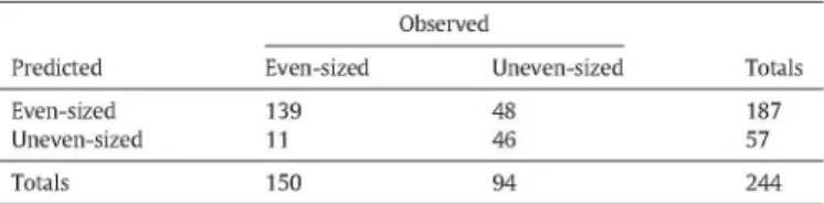
Concerning the classification results, using the Lev = 0.5 rule for dis-criminating even tree size (Seedling, Sapling, Young, Advanced and

Ma-ture) versus uneven tree size classes (Shelterwood, Seed-tree and Multi-storied) (Table 1), obtained an overall accuracy of 92.4% and a coefficient of agreement K = 0.48. A total of 92.7% of the even-sized plots were cor-rectly classified by this rule, with only few omission/commission errors. Most uncertainty was on the identification of uneven tree size forests, due to the inability for the Lev = 0.5 rule to identify Shelterwood areas (Fig. 1), as this rule only classified 24.4% of those areas as being un-even-sized.

4.2. L-skewness of ALS heights

The next step was to observe the capacity of Lskew to incorporate ad-ditional information about forest structure with regards to the relation-ships of relative dominance among the trees. Using the rule Lskew = 0 in Eq. (2) gives

L3 = 0. (8)

Therefore the rule is demonstrated directly by the zero value on the y-axis of the L3-L2 relation (horizontal dashed line in Fig. 2). In Fig. 2, we also observed a strong dependency of L3 on L2, since the spread of L3 values expands while L2 increases. This also illustrates the advan-tages of the Lskew ratio, which normalizes the L3 values of asymmetry, making them comparable among distributions of differing dispersion of ALS heights (hence, of different mean ALS height as well).

The utility of analysing the asymmetry of the ALS height distribu-tions was clear, as Lskew was associated with the capacity of penetration of the laser pulses, and therefore with the openness of the canopy. Pos-itive skewness (Lsfcew>0) was observed when there were large propor-tions of ALS returns with relatively lower heights, which indicates few dominant trees allow the laser beam to reach lower areas underneath an open upper canopy. On the other hand, negative skewness (Lskew -0) was observed when a closed dominant canopy backscatters most returns from the higher strata, and only few of them are returned from the understorey.

Regarding the discrimination of oligophotic (Young, Advanced

Ma-ture and Shelterwood,) and euphotic (Seedling, Sapling, Seed-tree and Multi-storied) areas of the forest (Table 2), the overall accuracy obtained was 84.6% and K = 0.56. These accuracies were quite large, considering a method making no use of field data, an indication that Lskew may be a good proxy for the degree of canopy closure.

Table 1

Direct rule Lev = 0.5. Contingency matrix of classification of even-sized versus uneven-sized development classes.

Fig. 1. Relationship between the first and the second moments of ALS heights (i.e., L-coefficient of variation).

Predicted

Even-sized Uneven-sized

Totals

Even-sized

139 11

150

Observed

Uneven-sized

48 46

94

Totals

187 57

c

E o E

<N

o

T

-3rt L-moment vs. 2nd L-moment

: Seedlings Saplings Young Advanced Mature

V Shelterwood

0 Seed-tree

* Multi-storied

a *

H

* B

* #

^ *

* » * 8 * B IS E ^

* * -a * *E *

* V *

B + V + * a V

w

o ^ *w

V

I I

L-skewness vs. L-coefficient of variation

2™ L-moment (L 2)

Fig. 2. Relationship between the second and third moments of ALS heights (i.e., L-skewness).

CM - J -*

v> « _

Is

9

a

80

/

+

*

VV j

+ V

I- * *

<>: x x

4-O

* v

Seedlings Saplings Young Advanced

Mature v Shelterwood

- Seed-tree * Multi-storied

0.2 0.4 0.6

L-coefficient of variation ( L 2 / L 1 ) — r

-0.8

Fig. 3. Relationship between the L-coefficient of variation and L-skewness of ALS heights.

4.3. Comparing rule-based versus supervised method

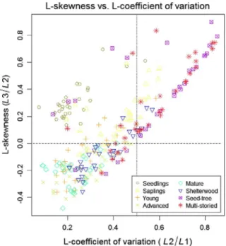
Fig. 3 shows a joint representation of both rules: Lev = 0.5 and

Lskew = 0, respectively represented by vertical dotted and horizontal

dashed lines. It therefore illustrates how these measures of relative dis-persion and asymmetry may be selected or combined in pursue of dif-ferent objectives for classifying forest structure and development directly from the distribution of ALS returns. Furthermore, we also com-pared all results with those obtained by a supervised classification car-ried out with this same subsample dataset. Tables 3 and 4 are contingency matrices for the aggregation of development classes (ac-cording to Section 3.2) predicted by the supervised SVM classification. For direct comparison, Table 5 includes a summary of results obtained by all the compared methods.

Regarding the results obtained from the supervised classification, it can be observed that the classification of forest areas into even and un-even tree sizes (Table 3) reached an overall accuracy 87.3% and K = 0.34, whereas oligophotic versus euphotic (Table 4) obtained overall ac-curacy of 93.8% and K = 0.80. Differences between the rule-based meth-od and the supervised approach were not so large if taking into account the simplicity and lack of involvement of field data in the former one. User's accuracies obtained by the SVM classification were very similar to those yielded by the rule-based method (Table 5), which demon-strates that they are mainly due to differences in the proportions of area that each development class has from the population, and not dif-ferences between the two methods. The success of the Lev = 0.5 thresh-old in classifying the even and uneven tree size forests and Lskew = 0 for segregating the oligophotic and euphotic areas of forest was remarkably good if compared to the supervised classification, which did not obtain much greater accuracies. The comparison of user's and producer's

accuracies against the supervised classification however highlighted the two major differences: the rule-based method increased the errors due to omission of uneven-sized areas and commission of euphotic areas (Table 5).

5. Discussion

5.1. L-coefficient of variation may identify tree size inequality

Our prior assumption was that forests with trees of approximately equal sizes - i.e., even tree size classes -, since they would backscatter most ALS returns from a single canopy stratum, could be directly detect-ed by low values of the Lev of their ALS heights. Our results corroborate this assumption, since 92.7% of the even tree size plots were correctly classified by this rule (blue colour in Fig. 4 examples). Fig. 3 shows that most uncertainty in even tree size areas - those containing trees of approximately equal sizes - was due to Sapling stands, whereas not one single plot belonging to either Advanced or Mature development classes showed values ofLcv>0.5. The low rate of omission errors im-plies that this rule could be used as a rather conservative and simple method when the purpose is to predict even tree size forest areas.

On the other hand, it was also expected that in the presence of struc-turally heterogeneous forests with more inequality of sizes among its trees, the ALS returns would also show a more spread pattern as they backscatter along the full vertical profile of the canopy, showing higher values of Lev. In view of our results, that was the case for Seed-tree and most Multi-storied areas, although not for Shelterwood stands. We there-fore propose that the direct rule Lcv> 0.5 may be used as an indicator of great tree size inequality only when regeneration is achieved by shade-intolerant species, and therefore it has been enabled by forest

Table 2

Direct rule lskew=0. Contingency matrix of classification of oligophotic (closed canopies) versus euphotic (open canopies) areas.

Table 3

Supervised classification. Aggregated classes from Valbuena et al. (2016b). Contingency matrix of classification of even-sized versus uneven-sized development classes.

Predicted

Oligophotic Euphotic

Observed

Oligophotic

102 19

Euphotic

17 106

Totals

119 125

Predicted

Even-sized Uneven-sized

Even-sized

131 19

Observed

Uneven-sized

15 79

Totals

146 98

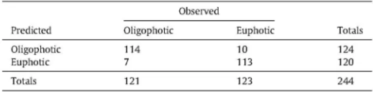
Table 4 _{5.2. L-skewness may identify fully closed canopies} Supervised classification. Aggregated classes from Valbuena et al. (2016b). Contingency

matrix of classification of oligophotic (closed canopies) versus euphotic (open canopies) areas.

Predicted

Oligophotic Euphotic

Totals

Oligophotic

114 7

121

Observed

Euphotic

10 113

123

Totals

124 120

244

disturbance (Knox et al., 1989; Kellner and Asner, 2009). In other words, a correspondence between the GC of tree sizes (Valbuena et al., 2013a) and the Lev of ALS heights may only happen when the large value of GC is due to the presence of a gap in the canopy, which allows a large pro-portion of the laser footprint to get through and disperse its correspond-ing returns along the vertical profile of the canopy (Stark et al., 2012). This highlighted the importance of employing an additional metric dis-criminating areas with a large euphotic zone from those where regener-ation occurs in the oligophotic zone (Lefsky et al., 2002; Fig. 5). Whether or not more ALS metrics are required for fully describing the structural properties of forests, it is worth noting the recurrence of Lev as a variable selected by many different automated methods tested in our previous studies, and therefore the role of Lev in predicting structural attributes related to tree size inequality (Valbuena et al., 2013b, 2014, 2016a) and forest development (Valbuena et al., 2013a, 2016b) seems clear.

Exploring the reasons why only 24.4% of Shelterwood stands were classified by the Lcv>0.5 rule as being uneven-sized, it could be taken into account that this development class was also the one showing most error in the SVM classification (Valbuena et al., 2016b). The fact that a supervised method, which used the explanatory potential of many other metrics as well, still failed to reliably identify Shelterwood areas may be an indication that the limitation is due not to the metrics but rather to the original ALS data. Due to the low-density nature of this national dataset (NLS, 2013), the laser footprint probably detects very infrequently the presence of understory under closed dominant canopies. In that case, scan density would need to be increased for this task. We considered the advantages of testing the rule-based method with this type of ALS dataset since, due to its simplicity, could have po-tential for replication at national scales. Further research should, how-ever, employ datasets of larger densities to clarify whether Lev could then show better capacity for detecting regeneration of shade-tolerant species. If direct replication of the rule-based method is to be envisaged, the effect of other flight parameters in these L-moment ratios, such as scanner device or maximum scanning angle (Nassset, 2004; Disney et al., 2010), should also be object of future investigations.

Table 5

Comparison of accuracy results.

Stratification

Even vs. Uneven tree size Overall accuracy {OA) Kappa (K)

Even tree size omission {PA) Even tree size commission {UA) Uneven tree size omission {PA) Uneven tree size commission {UA) Oligophotic vs. Euphotic Overall accuracy {OA) Kappa (K)

Oligophotic omission {PA) Oligophotic commission {UA) Euphotic omission {PA) Euphotic commission {UA)

Rule-based classification

Lev = 0.5 92.4% 0.48 92.7% 99.6% 48.9% 4.2% Lskew = 0 84.6% 0.56 84.3% 96.8% 86.2% 52.9%

Supervised classification3

SVM 87.3% 0.34 87.3% 99.8% 84.0% 4.1% SVM 93.8% 0.80 94.2% 98.3% 91.9% 76.8%

a Aggregated from Valbuena et al. (2016b).

The threshold derived from the asymmetry measure of L-moments, Lskew = 0, was demonstrably practical with regards to discriminating oligophotic from euphotic areas. Lskew<0 denotes areas where most ALS returns were backscattered from a closed dominant canopy which only allows small proportions of the laser footprint - and the light re-source - to reach the understorey. Conversely, Lskew>0 was observed whenever there were large proportions of ALS heights with relatively lower heights, and it was therefore related to the presence of only few returns backscattered from upper areas in the canopy, which indicates that the dominant trees allow the laser beam - and thereby the light re-source - to reach lower areas underneath an open canopy. This can be rel-evant with regards to findings by Drake et al. (2002) and Lefsky et al. (2005), who found the degree of canopy closure to be one of the most rel-evant covariates in the relation between biomass and ALS heights.

It may be worth noting that the Lskew> 0 rule was capable of practical-ly delineating Seedling, Sampling and Seed-tree stands directpractical-ly (Fig. 4). Al-though the method was carried out at pixel-level, the resulting maps identified entire stands sharply. The rule-based stratification by Lskew>0 was therefore fairly insensitive to the within-stand variation that usually makes it difficult to discriminate stands, especially Seed-tree areas, by standard area-based procedures in remote sensing. These types of prob-lems usually require more complex analyses at object-level - representing stands -, which involve segmentation procedures with subjective steps, parameters determined by trial-and-error, or manual delineation (e.g., Pascual et al., 2008). In contrast, the rule based method offers a simple procedure to determine Seedling, Sampling and Seed-tree stands directly.

5.3. Synergies between the rules

Overall accuracies obtained by the rule-based methods were, re-spectively, 92.4% and 84.6% which we considered a remarkable achieve-ment for a rule-based method not requiring field support for training and that they were comparable to the results obtained by the super-vised classification (87.3% and 93.8%, respectively; Table 5). As a rule of thumb, it may be affirmed that Lskew>0 characterizes canopies not fully closed (areas not having reached stem exclusion), whereas those areas which also had values of Lcv>0.5 presented large inequality among tree sizes driven by forest disturbance (Fig. 5). In our results in Fig. 3, values of wide dispersion Lcv>0.5 occurred only in the presence of positive skewness Lskew>0. This was also corroborated out of the sample, as pixels with Lcv>0.5 also had Lskew>0 as well (Fig. 4). This demonstrates that, in these low-density datasets, the variance of ALS heights only increases as a cause of openness in the canopy and an in-crease of the euphotic zone (Lefsky et al., 2002), possibly due to forest disturbance, which leads to positive skewness in the distribution. As a consequence, the maps obtained with Lcv> 0.5 were expanded by the

Lskew>0 rule (Fig. 4), extending the areas of large tree size inequality towards those simply presenting potential for growth with no limita-tion from light resource. In turn, negatively skewed Lskew< 0 ALS height distributions (Fig. 2) are indicative of forests with large oligophotic zone (Lefsky et al., 2002) and therefore can only allow the regeneration of shade-tolerant species. It is worth commenting that uneven tree size and euphotic forest areas stand out of a general relationship between first moments of ALS heights and forest attributes related to mean diam-eter (Lefsky et al., 2002, 2005), and therefore we suggest that one po-tential use of the rule-based method could be to decrease the signal-to-noise ratio when obtaining ALS-assisted estimations in heteroge-neous forest areas.

5.4. Practical benefits and further research needs

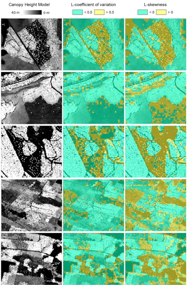
Canopy Height Model L-coefficient of variation L-skewness

40 m 0 m < 0.5 > 0 . 5 < 0 > 0

Fig. 4. Examples of resulting maps of forests stratified with rule-based method. Left: canopy height model (CHM). Middle: areas with Lcv>05 in yellow (uneven tree sizes) and Lcv<0.5 in blue (even tree sizes). Right: areas with Lskew> 0 in yellow (euphotic) and Lskew<0 in blue (oligophotic). The reference CHM was made from the same ALS dataset, courtesy of Aid Suvanto (Blom Kartta Oy).

Lskew = 1

£

e o

13

Euphotic A A

A^ A J i l A J ^ -1^

• A+AiA

^ < ^ =

-

-m

EQUALITY ON JREE SIZES

Inequal

Lskew = -1 Lev = 0*

Lev-L-coefficient of variation •

0,5

Gini Coefficient (spread) -» Lcv= 1

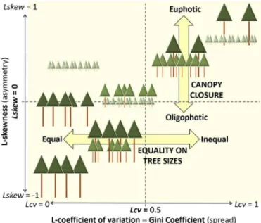
Fig. 5. Schematic diagram representing the patterns of ALS return distribution that can be

found in different types of forest structures, and how they are described by ratios of

L-moments: L-coefficient of variation and L-skewness. Compare to Fig. 3 and Valbuena et

al. (2013a: Fig. 4).

for describing light availability conditions (Lefsky et al., 2002), forest disturbance characteristics (Kellner and Asner, 2009), or tree growth (Stark et al., 2012) and regeneration (Valbuena et al., 2013a). Further research should clarify the role of different flight configurations, scan-ners systems or scanning density (Nassset, 2004; Disney et al., 2010) in the relationships between ALS L-moments and forest structural characteristics.

The resulting classification could be used e.g. in stratification of a for-est area for the field data collection of an ALS inventory campaign, since Hawbaker et al. (2009), Maltamo et al. (2011) and Gobakken et al. (2013) demonstrated that a field sampling strategy based on a priori knowledge extracted from the ALS itself may be advantageous. In the presence of within-stand heterogeneity (e.g., Valbuena et al., 2013a), L-moments could be valuable for delineating microstands (van Aardt et al., 2006). There are potential applications in guiding future forest management operations directly from ALS datasets, once unveiling the relationship between GC and silvicultural alternatives (Pukkala et al., 2016) and thereby to L-moments of ALS returns. For ecosystem studies, there is potential for studying canopy structure, e.g., discrimination of single- and multi-layered forests, and other traits relevant to old-growth forests (Lefsky et al., 2002; Miura and Jones, 2010). We encour-age further research to exploit the potential of L-moments in forest estimation (e.g., Asner and Mascaro, 2014) and other applications.

6. Conclusions

We developed a rule-based classification deduced from L-moments summarizing the relative dispersion and skewness of ALS heights. Clas-sification by two simple deductive mathematical rules, L-coefficient of variation Lcv>0.5 and L-skewness Lskew>0, was carried out directly on the ALS return cloud, omitting training stages making use of field plot data. Lev was related to tree size inequality, while Lskew provided information on the degree of closure of the dominant canopy. These provide relevant information about competition conditions in different areas of the forest, which can be deduced directly from ALS datasets. Our conclusions, however, may apply only to Boreal ecosystems, where light availability and its interception by the dominant canopy is the compet-itive process that limits forest growth. Some of the accuracies obtained were remarkably large, being a direct classification using no field data support, and they were comparable to those obtained by a supervised

classification. Two flaws of the rule-based method were the omission of uneven-sized forest with shade-tolerant regeneration and commis-sion errors for the euphotic areas, to be solved by further research per-haps making use of datasets with higher density. These rules can be executed directly over ALS datasets, providing an unambiguous proce-dure with multiple applications.

Acknowledgements

This research was funded by Suomen Metsakeskus (SMK Finnish Forest centre). Special thanks to Juho Heikkila and Jussi Lappalainen (SMK), Heli Laaksonen (NLS), and Aki Suvanto (Blom Kartta Oy) for their support at different stages of this study. Ruben Valbuena would like to thank The Finish Society of Forest Sciences for awarding a IUFRO Grant which sponsored his travel to present this work at Silvilaser 2015 Conference in La Grande Motte (France). Special issue editors are thanked for inviting this communication and three anony-mous reviewers for their helpful and constructive comments.

Appendix A. L-moments and their relationship to Gini Coefficient

A. 1. L-moments for describing a distribution

Let an order statisticXfcr be the fc-th smallest observation in a sample of size r of the random variable X (e.g. ALS return heights), and let £(Xfcr) be its expected value. For example, consider £(Xi:2) in the following population of size 3: {12,16,14}. There are three possible samples of size r = 2, with sample minima (k= 1): {12,12,14}. The expected value is the mean over these, i.e., £(Xi:2) = 12.67. In the analysis of this paper, the population is the unknown infinite set of all possible ALS returns over the primary calculation unit (sample plot or grid cell). The expected value is estimated using the observed sample of returns.

L-moments describe the distribution of a scalar random variable X through weighted sums of £(Xfcr). Hosking (1990) defined the L-mo-ments as:

I^r"

£ ( - ! ) * ( V )£(X

_

).

The first L-moment (LI) is obtained by substituting r = 1 in Eq. (Al) to get:

I1=£(X1 : 1)=£(X), (A2)

which is thus equivalent to the first product-moment (expectation) of X Hence, LI is the L-measure for the location or central tendency of the distribution. If observations of X are available, LI can be estimated as the arithmetic mean:

L\ = X.

second L-moment (L2), follows the case for r = 2: The

L2=^E(X2:2)-^E(X1:2)=^E[X2:2-X,

(A3)

(A4)

which is the expected value of half difference between minimum (Xi:2) and maximum (X2:2) in a sample of size two. It therefore provides the mean of half differences, and thus it is the L-measure for the dispersion of the distribution.

Following a similar logic for the third L-moment (L3), substituting r = 3 in Eq. (Al) yields:

L3 =^£(X3 :3)-|£(X2 : 3) +^£(X1:3), (A5)

maximum (X3:3) of a sample with size three. It can further be written as: of individuals in the population. From Eq. (A9), Kleiber (2005: Eq. 6) showed that:

L3 = ^£[(X3:3--X-23) — (X2;3— Xl;3)]. (A6)

to show that L3 expresses the expected difference between the maxi-mum-median and median-minimum differences in a sample of size three, which provides a L-measure for the asymmetry of the distribution ofX Hence, L3 = 0 corresponds to a symmetric distribution, L3>0 scribes positive asymmetry (left-skewed distribution) and L3<0 de-scribes negative asymmetry (right-skewed distribution).

A.2. L-moment ratios

Hosking (1990) also defined the ratios for L-moments. They have the advantage of being bounded by finite intervals (Hosking, 1989), yield-ing comparable relative descriptions for the distribution ofX

The second L-moment ratio is obtained as the ratio of the second to the first L-moments. It is called the L-coefficient of variation (Lev) for its comparison to conventional moments. From Eqs. (A2) and (A4) it can be observed that Lev equals:

12 £(X2:2)-£(X1:2)

2£(X) (A7)

For positive random variables, the values for the second L-moment ratio are bounded by the [0,1 ] range (Hosking, 1989). Just like the coef-ficient of variation of conventional moments, Lev is a descriptor of dis-persion relative to central tendency; that is to say, concentration. This brings the advantage that concentration measures are comparable among distributions differing in their location or central tendency (LI), and also independently of the units of measure. It is worthwhile to note that Hosking never defined a second L-moment ratio, as their generalized definition stands only for r = 3,4... (Hosking, 1990: 108), and the L-coefficient of variation was simply presented alongside. It was only later that many authors have regarded Lev to be the second L-moment ratio.

The third L-moment ratio is obtained by division between the third and the second L-moments. It is called the L-skewness (Lskew), as it has been found to be a robust descriptor for the asymmetry of the distri-bution ofX From Eqs. (A4) and (A6), and using the equivalence£(X3:3 -X1:3) = |£(X2 : 2-X1 : 2)(Robbins, 1944: Eq. 22; David and Nagaraja, 2003:44, 56) it yields:

Lskew • L3_£(X3:3)-2£(X2:3)+£(X1:3)

L2 £(X3:3)-£(X1:3) (A8)

As explained for L3, Lskew = 0 corresponds to a symmetric distribu-tion, while positive or negative values denote the type of asymmetry for the distribution. Additionally, Lskew has the advantage of presenting theoretical bounds within the [—1,1] interval (Hosking, 1989). Conse-quently, Lskew is a descriptor of asymmetry relative to dispersion, and therefore independent of the units of measure and the dispersion of the distribution of X

A3. Equivalence between the Cini coefficient and the L-coefficient of variation

The Gini coefficient of a scalar random variable X(GC) is the ratio of the area comprised between the Lorenz curve and the diagonal line of equality (Gini, 1921):

GC = 1 -2jlHX)dX: _(A9)

where L(X) is the Lorenz curve: the relative cumulative distribution of a variable against the cumulative frequency distribution of the proportion

GC = 1- £(X1:2)

£(X) ' (A10)

Lev =

On the other hand, the Lev gives also the GC. From Eq. (A7) it derives:

£(X2:2)-£(X1:2) 2£(X)

£(X2:2-X1:2) + 2£(X1:2)-2£(X1:2) 2£(X)

£(X2:2+X1:2)-2£(X1:2) 2£(X)

2£(X)-2£(X1:2) 2£(X)

= 1- £(X1:2) £(X) '

(Alia)

(Allb)

(Allc)

(Alld)

(Alle)

Eq. (Alld) results from (Allc) because X1:2+X2:2 is the sum of two independent and identically distributed samples, and it is therefore equivalent to Xi +X2. Consequently, Eqs. (A10) and (Alle) demon-strate:

GC = Lev. (A12)

The result in Eq. (A12) is essentially a special case of a 140-years-old result (Helmert, 1876; as cited in David and Nagaraja, 2003: 249) pre-sented in equation 9.4.2 of David and Nagaraja (2003), which might even provide interesting extensions using expectations of order statis-tics in sample sizes larger than r = 1,2,3.

Appendix B. Criteria for determining forest development classes

Silvicultural development classes are used in Finland to classify for-est stands and assist in decision-making for forfor-est management plan-ning. It was possible to apply stratified sampling using the stand register dataset employed by the Finnish Forest Centre (SMK, Suomen Metsakeskus) for their operational management planning, since a de-velopment class has been explicitly assigned to each stand from previ-ous inventories. The development class to which each sample plot belonged to was nevertheless ultimately corroborated in the field, being the criteria used in-situ prevalent over the stand register data. Minor differences in per-stratum sample sizes were simply caused by such type of discrepancies found in few plots. The criteria that segregat-ed forest areas into different forest classes were:

• Seedling: stands with average tree height<0.10 1.3 m, and absence of mature trees (overstorey).

• Sapling: stands with average tree height > 1.3 m, and average diameter at breast height (DBH)<0.10 8 cm, and absence of mature trees (overstorey).

• Young: stands with average DBH ranging 8-16 cm and average tree height ranging 7-9 m high.

• Advanced: stands with average DBH > 16 cm

• Mature: stands reaching a quadratic mean DBH (QMD) > 18 cm. • Shelterwood: stands including a dense overstorey of mature trees

(DBH > 16 cm) which reaches at least 100-300 stemsha- 1, and also a dense understorey of seedlings (height < 1.3 m) of shade-tolerant species, usually Norway spruce (1500-1800 stemsha- 1).

pine (1500-2200 stems-ha-1) or Birch species (1100-1600 stems-ha-1).

• Multi-storied: stands including a dense understorey (above-men-tioned densities) of seedlings (height < 1.3 m) and saplings (height > 1.3 m, DBH < 8 cm) of any species, usually deciduous but also Scots pine or Norway spruce. The size of trees in the overstorey is not a determinant criterion, but trees in the understory must reach their sapling stage.

References

Asner, G.P, Mascara, J., 2014. Mapping tropical forest carbon: Calibrating plot estimates to a simple LiDAR metric. Remote Sens. Environ. 140,614-624.

Bollandsas, O.M., Naesset, E, 2007. Estimating percentile-based diameter distributions in uneven-sized Norway spruce stands using airborne laser scanner data. Scand. J. For. Res. 22, 33-47.

Cohen, J, 1960. A coefficient of agreement for nominal scales. Educ Psychol. Meas. 20 (1), 37-46.

Cordonnier, T., Kunstler, G, 2015. The Gini index brings asymmetric competition to light Perspect Plant Ecol. Evol. Syst 17 (2), 107-115.

Dalponte, M., Bruzzone, L, Gianelle, D., 2008. Fusion of hyperspectral and LIDAR remote sensing data for classification of complex forest areas. IEEE Trans. Geosci. Remote Sens. 46 (5), 1416-1427.

David, H.A, Nagaraja, H.N, 2003. Order Statistics. Wiley Series in Probability and Statis-tics, third edition John Wiley, New York

Disney, M.I, Kalogirou, V, Lewis, P., Prieto-Blanco, A, Hancock S., Pfeifer, M, 2010. Simu-lating the impact of discrete-return lidar system and survey characteristics over young conifer and broadleaf forests. Remote Sens. Environ. 114,1546-1560. Drake, J.B., Dubayah, RO., Knox, RG., Clark, D.B, Blair, J.B., 2002. Sensitivity of

large-foot-print lidar to canopy structure and biomass in a neotropical rainforest Remote Sens. Environ. 81 (2-3), 378-392.

Frazer, G.W., Wulder, M.A, Niemann, K.O., 2005. Simulation and quantification of the fine-scale spatial pattern and heterogeneity of forest canopy structure: A lacunarity-based method designed for analysis of continuous canopy heights. For. Ecol. Manag. 214 (1-3), 65-90.

Frazer, G.W., Magnussen, S, Wulder, MA, Niemann, K.O., 2011. Simulated impact of sam-ple plot size and co-registration error on the accuracy and uncertainty of LiDAR-de-rived estimates of forest stand biomass. Remote Sens. Environ. 115,636-649. Garcia, M., Riano, D., Chuvieco, E, Salas, J., Danson, F.M., 2011. Multispectral and LIDAR

data fusion for fuel type mapping using support vector machine and decision rules. Remote Sens. Environ. 115 (6), 1369-1379.

Gini, C, 1921. Measurement of inequality of incomes. Econ. J. 31,124-126.

Gobakken, T, Korhonen, L, Naesset, E, 2013. Laser-assisted selection of field plots for an area-based forest inventory. Silva Fenn. 47 (5), 943.

Gove, J.H, 2004. Structural stocking guides: A new look at an old friend. Can. J. For. Res. 34, 1044-1056.

Hall, SA, Burke, I.C, Box, D.O, Kaufmann, M.R, Stoker, J.M., 2005. Estimating stand struc-ture using discrete-return lidar: An example from low density, Are prone ponderosa pine forests. For. Ecol. Manag. 208 (1-3), 189-209.

Hawbaker, T.J., Keuler, N.S., Lesak, AA, Gobakken, T, Contrucci, K., Radeloff, V.C, 2009. Improved estimates of forest vegetation structure and biomass with a LiDAR-opti-mized sampling design. J. Geophys. Res. 114, G00E04.

Helmert, F.R, 1876. Die Berechnung des wahrscheinlichen Beobachtungsfehlers aus den ersten Potenzen der Differenzen gleichgenauer director Beobachtungen. Astron. Nachr. 88,127-132.

Hosking, J.RM, 1989. Some theoretical results concerning L-Moments. Research Report RC14492. IBM research, Yorktown Heights.

Hosking, J.RM., 1990. L-moments: Analysis and estimation of distributions using linear combinations of order statistics. J. R Stat Soc. Ser. B Methodol. 52,105-124. Jaslaerniak, D., Lane, P.N.J., Robinson, A., Lucieer, A, 2011. Extracting LiDAR indices to

characterise multilayered forest structure using mixture distribution functions. Remote Sens. Environ. 115, 573-585.

Kellner, J.R., Asner, G.P., 2009. Convergent structural responses of tropical forests to diverse disturbance regimes. Ecol. Lett 12,887-897.

Kleiber, C, 2005. The Lorenz curve in economics and econometrics. Invited Paper, Gini-Lo-renz Centennial Conference, Siena (Italy).

Knox, RG, Peet, RK, Christensen, N.L, 1989. Population dynamics in loblolly pine stands: Changes in skewness and size inequality. Ecology 70,1153-1167.

Lefsky, MA, Cohen, W.B, Acker, SA, Spies, TA, Parker, G.G, Harding, D, 1999a. Lidar re-mote sensing of biophysical properties and canopy structure of forest of Douglas-fir and western hemlock Remote Sens. Environ. 70, 339-361.

Lefsky, MA, Harding, D, Cohen, W.B, Parker, G, Shugart, H.H, 1999b. Surface lidar re-mote sensing of basal area and biomass in deciduous forests of eastern Maryland, USA. Remote Sens. Environ. 67, 83-98.

Lefsky, MA, Cohen, W.B, Parker, G, Harding, D, 2002. Lidar remote sensing for ecosys-tem studies. Bioscience 52,19-30.

Lefsky, MA, Hudak AT, Cohen, W.B, Acker, SA, 2005. Patterns of covariance between forest stand and canopy structure in the Pacific Northwest. Remote Sens. Environ. 95,517-531.

Maltamo, M, Packalen, P, Yu, X, Eerikainen, K, Hyyppa, J, Pitkanen, J, 2005. Identifying and quantifying structural characteristics of heterogeneous boreal forests using laser scanner data. For. Ecol. Manag. 216,41-50.

Maltamo, M, Bollandsas, O.M, Naesset, E, Gobakken, T, Packalen, P, 2011. Different plot selection strategies for field training data in ALS-assisted forest inventory. Forestry 84, 23-31.

Meyer, D, Dimitriadou, E, Hornik, K, Weingessel, A, Leisch, F, 2014a. el071: Misc Func-tions of the Department of Statistics, TU Wien. R package version 1.6^1 (http://ugrad. statubc.ca/RAibrary/el071/html/00Index.html. Visited in Jan. 2014).

Meyer, D, Zeileis, A, Hornik K, 2014b. vcd: Visualizing Categorical Data. R package ver-sion 1.3-2 (https://cran.r-prqjectorg/web/packages/vcd/index.html Visited in Jan. 2014).

Miura, N, Jones, S.D, 2010. Characterizing forest ecological structure using pulse types and heights of airborne laser scanning. Remote Sens. Environ. 114 (5), 1069-1076. Naesset, E, 2002. Predicting forest stand characteristics with airborne scanning laser using

a practical two-stage procedure and field data. Remote Sens. Environ. 80, 88-99. Naesset, E, 2004. Effects of different flying altitudes on biophysical stand properties

esti-mated from canopy height and density measured with a small-footprint airborne scanning laser. Remote Sens. Environ. 91 (2), 243-255.

NLS - National Land Survey of Finland 2013. Laser scanning data available online at

maanmittauslaitos.fi. (Visited in Sep. 2013).

Olofsson, P, Foody, G.M, Stehman, S.V, Woodcock C.E, 2013. Making better use of accu-racy data in land change studies: Estimating accuaccu-racy and area and quantifying un-certainty using stratified estimation. Remote Sens. Environ. 129,122-131. Ozdemir, I, Donoghue, D.N.M, 2013. Modelling tree size diversity from airborne laser

scanning using canopy height models with image texture measures. For. Ecol. Manag. 295,28-37.

Pascual, C, Garcia-Abril, A, Garcia-Montero, LG, Martin-Fernandez, S, Cohen, W.B, 2008. Object-based semi-automatic approach for forest structure characterization using lidar data in heterogeneous Pinus sylvestris stands. For. Ecol. Manag. 255 (11), 3677-3685.

Pontius, RG, Santacruz, A, 2015. diffeR: Metrics of Difference for Comparing Pairs of Maps. R package version 0.0-4 (http://CRAN.R-project.org/package=diffeR Visited in Apr. 2016).

Pukkala, T, Laiho, O, Lahde, E, 2016. Continuous cover management reduces wind dam-age. For. Ecol. Manag. 372,120-127.

Robbins, H.E, 1944. On the expected values of two statistics. Ann. Math. Stat 15,321-323. Stark, S.C, Leitold, V, Wu, J.L, Hunter, M.O, de Cashlho, C.V, Costa, F.R, McMahon, S.M, Parker, G.G, Shimabukuro, M.T., Lefsky, MA, Keller, M, Alves, L.F, Schietti, J, Shimabukuro, YE, Brandao, D.O, Woodcock T.K, Higuchi, N, de Camargo, P.B, de Oliveira, R.C, Saleska, S.R, Chave, J, 2012. Amazon forest carbon dynamics predicted by profiles of canopy leaf area and light environment Ecol. Lett 15 (12), 1406-1414 Stehman, S.V, 1996. Estimating the kappa coefficient and its variance under stratified

random sampling. Photogramm. Eng. Remote Sens. 62 (4), 401-402.

Valbuena, R, Packalen, P, Martin-Fernandez, S, Maltamo, M, 2012. Diversity and equita-bility ordering profiles applied to study forest structure. For. Ecol. Manag. 276, 185-195.

Valbuena, R, Packalen, P, Mehtatalo, L, Garda-Abril, A, Maltamo, M, 2013a. Characteriz-ing forest structural types and shelterwood dynamics from Lorenz-based indicators predicted by airborne laser scanning. Can. J. For. Res. 43,1063-1074

Valbuena, R, Maltamo, M, Martin-Fernandez, S, Packalen, P, Pascual, C, Nabuurs, G.J, 2013b. Patterns of covariance between airborne laser scanning metrics and Lorenz curve descriptors of tree size inequality. Can. J. Remote. Sens. 39, S18-S31. Valbuena, R, Vauhkonen, J, Packalen, P, Pitkanen, J, Maltamo, M, 2014. Comparison of

airborne laser scanning methods for estimating forest structure indicators based on Lorenz curves. ISPRS J. Photogramm. Remote Sens. 95,23-33.

Valbuena, R, Eerikainen, K, Packalen, P, Maltamo, M, 2016a. Gini coefficient predictions from airborne lidar remote sensing display the effect of management intensity on for-est structure. Ecol. Indie. 60,574-585.

Valbuena, R, Maltamo, M, Packalen, P, 2016b. Classification of multi-layered forest de-velopment classes from low-density national airborne lidar datasets. Forestry 89, 392-401.

van Aardt, JAN, Wynne, RH, Oderwald, RG, 2006. Forest volume and biomass estima-tion using small-footprint LiDAR-distribuestima-tional parameters on a per-segment basis. For. Sci. 52 (6), 636-649.

Wang, QJ., 1996. Direct sample estimators of L moments. Water Resour. Res. 32 (12), 3617-3619.

Weiner, J, 1990. Asymmetric competition in plant populations. Trends Ecol. Evol. 5, 360-364.

Westfall.JA, Patterson, P.L, Coulston, J.W, 2011. Post-stratified estimation: Within-strata and total sample size recommendations. Can. J. For. Res. 41 (5), 1130-1139. White, J.C, Wulder, MA, Varhola, A, Vastaranta, M, Coops, N.C, Cook, B.D, Pitt, D,

Woods, M, 2013. A best practices guide for generating forest inventory attributes from airborne laser scanning data using an area-based approach. Natural Resources Canada, Information Report FI-X-010. Canadian Forest Service, Victoria, BC Zenner, E.K, 2005. Development of tree size distributions in Douglas-fir forests under

dif-fering disturbance regimes. Ecol. Appl. 15, 701-714.