Characteristics of the turbulent/nonturbulent
interface in boundary layers, jets and shear-free
turbulence
Carlos B. da Silva1, Rodrigo R. Taveira1, Guillem Borrell2 1Department of Mechanical Engineering. Instituto Superior T´ecnico. Lisboa. Portugal 2
ETSI Aeron´auticos. Universidad Polit´ecnica de Madrid. Madrid. Spain
E-mail: [email protected]
Abstract. The characteristics of turbulent/nonturbulent interfaces (TNTI) from boundary layers, jets and shear-free turbulence are compared using direct numerical simulations. The TNTI location is detected by assessing the volume of turbulent flow as function of the vorticity magnitude and is shown to be equivalent to other procedures using a scalar field. Vorticity maps show that the boundary layer contains a larger range of scales at the interface than in jets and shear-free turbulence where the change in vorticity characteristics across the TNTI is much more dramatic. The intermittency parameter shows that the extent of the intermittency region for jets and boundary layers is similar and is much bigger than in shear-free turbulence, and can be used to compute the vorticity threshold defining the TNTI location. The statistics of the vorticity jump across the TNTI exhibit the imprint of a large range of scales, from the Kolmogorov micro-scale to scales much bigger than the Taylor scale. Finally, it is shown that contrary to the classical view, the low-vorticity spots inside the jet are statistically similar to isotropic turbulence, suggesting that engulfing pockets simply do not exist in jets.
1. Introduction
In many turbulent shear flows such as boundary layers, jets, mixing layers and wakes there is a sharp interface that divides the flow field into two distinct regions. In one region the flow is turbulent while in the other, the flow is largely irrotational (Corrsin and Kistler [1]). This sharp interface - the turbulent/nonturbulent interface (TNTI) – is continually deformed over a wide range of scales and the flow dynamics in its vicinity determines many of the most important flow features: the growth and spreading rate of wakes, the exchanges of mass across mixing layers, and the mixing and reaction rates in jets are some of the flow features that are largely determined by the characteristics of the TNTI and the flow dynamics in its vicinity.
The key event that occurs at a TNTI is the ‘communication’ of vorticity from the core of the turbulent region into the irrotational zone. Turbulent entrainment can be seen as the mechanism by which fluid elements from the irrotational flow region acquire vorticity and become part of the turbulent region. Past studies described the entrainment as being caused by large-scale eddy motions (engulfment) occurring from time to time at particular locations along the TNTI [2], but recent works suggest instead that the entrainment results from small scale motions (nibbling) acting along the entire TNTI (Mathew and Basu [3], Hunt et al.[4]), as originally described by Corrsin and Kistler [1].
The flow dynamics near the TNTI has been assessed in several recent works and it has been observed that many flow variables, e.g., velocity and vorticity display characteristic (sharp) jumps at the TNTI (Westwerweel et al. [5], Holzneret al. [6], da Silva and Pereira [7]), and the dynamics of the vorticity and kinetic energy have been analysed near the TNTI to understand these jumps (e.g. Holzneret al. [6], Taveira and da Silva [8], Taveiraet al. [9]).
Links between geometry and dynamics are often not straightforward, but several studies have addressed the geometrical characteristics of TNTIs from different flows. It is know from numerous experimental observations that the TNTI is sharp and is continually distorted at a large range of scales by the turbulent structures in its vicinity (Corrsin and Kistler [1], Townsend [2]). The largest convolutions observed at the TNTI are the imprint of the largest-scale eddies from the turbulent region, which move at a speed imposed by their characteristic velocity and the integral scaleL11from the turbulent region (Townsend [10]). Statistics of the TNTI position
yi were assessed in numerous works starting with Corrsin and Kistler [1]. They concluded that
yi is approximately Gaussian, a result that has been remarked in numerous works since then
e.g. Gampert et al. [11]. However, La Rue and Libby have measured the forward and backward slopes of the TNTI using experimental data in the wake of a heated cylinder, and observed that these slopes are different, which is inconsistent with Gaussian distribution ofyi. The convex and
concave regions of the TNTI were assessed recently in experimental turbulent jets by Wolfet al.
[12] and it was realised that depending on the surface shape, different small-scale mechanisms are dominant for the local entrainment process.
The geometry of the TNTI has also been linked to the flow structures underneath e.g. da Silva and Reis [13] analysed the coherent vortices near the TNTI and observed that large vortical structures are responsible for the existence of positive enstrophy diffusion along the interface layer, linking the results of Holzner et al. [6] to the large-scale vorticity structures. Moreover, the characteristic vorticity jump observed in different flows has been linked to the eddy structure near the TNTI (da Silva and Taveira [14]), and the dynamics of the small-scale intense vorticity structures neighbouring the TNTI suggests that the nibbling eddy motions are linked to the diffusion of vorticity from these small scale vortices near the TNTI (da Silva et al. [15]).
Another geometrical feature of the TNTI is its fractal character. Indeed, the appealing idea that turbulence exhibits a scale-invariant (or fractal) character has lead to much research fired by the new ideas beautifully presented by Mandelbrot [16]. Numerous past experimental and some numerical works have searched for the (self-similar) fractal features of lines and surfaces within turbulent flows. The TNTI defined using the vorticity or a passive scalar supported the existence of a range of scales exhibiting self-similar fractal dimension between D2 ≈2.3−2.4 in numerous different flows (Sreenivasan [17]). However, many works have also raised doubts on the self-similar character, suggesting instead a more complex scale-dependent fractal dimension
i.e. multifractal behaviour for some variables (Frederiksenet al. [18], Catrakis [19]), but recent work based on experimental data from boundary layers is consistent with the TNTI being a self-similar fractal withD2 ≈2.3−2.4 (de Silvaet al. [20]).
Even though several geometrical aspects of TNTI have been analysed in the past, no systematic work addressed the differences and similarities from TNTIs in different flows. This work presents a first attempt at such a study. The data banks analysed here comprise direct numerical simulations (DNS) of boundary layers, planar jets and shear-free turbulence. In all the simulations, the Reynolds number based on the Taylor micro-scale is slightly greater than
Reλ ≈ 100, the main differences being the boundary and initial conditions, the existence or
absence of mean shear, or the proximity of the mean shear to the location of the TNTI.
Figure 1: Sketch of the simulation, presenting the dual configuration with an auxiliary boundary layer.
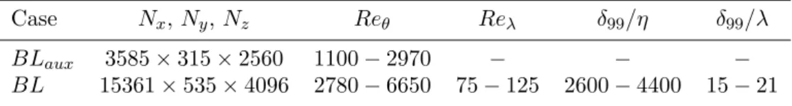
Case Nx,Ny,Nz Reθ Reλ δ99/η δ99/λ
BLaux 3585×315×2560 1100−2970 − − −
BL 15361×535×4096 2780−6650 75−125 2600−4400 15−21
Table 1: Parameters of the boundary layer simulation. Nx,Ny andNz are the computational domain
size. The following columns correspond to the values at the beginning and at the end of the simulation domain that is considered correct. Given that both the Kolmogorov (η) and Taylor (λ) scales change depending on the distance to the wall, a reference height y= 0.6δ99 has been chosen.
layers and jets. Section 5 compares the intermittency characteristics and associated length scales in the three flows analysed here, while section 6 discusses the thickness of the local vorticity jump in jets. Finally, in section 7 the geometry of the irrotational bubbles that are found inside a jet is investigated. The work ends with an overview of the main results and conclusions (section 8).
2. Description of the data sets
All the data used in this study have been obtained from Direct Numerical Simulation (DNS). Thanks to recent advances in particle image velocimetry [21] (PIV), and particle tracking velocimetry [6] (PTV), experimental techniques are able to capture the interface with accuracy, and to obtain the properties of the flow at the same time, but one important advantage of DNS over experimental techniques is its dynamic range, and in consequence, the ability to capture all the relevant scales in each case. Given that the goal of this study is to compare the geometrical properties of the interface detection in different flows, DNS data are a more reasonable choice.
Capturing all the information contained in the field comes with a cost. The separation between the smallest scales, given by viscosity, and the largest ones, given by the geometry of the problem, is proportional to the computational cost. Knowing that scale separation is crucial in the analysis of turbulent flows, this study uses some of the largest simulations available today.
2.1. Boundary layer
In the boundary layer, the streamwise, wall-normal, and spanwise directions are calledx,y, andzrespectively. Only the principal simulationBLis used. A list of the important parameters of the dataset is presented in table 1. Detailed statistics, that agree perfectly with the previous experiments and simulations, can be found in Sillero and Jim´enez [24], where a detailed analysis of the convergence of the large scales can be found.
It is important to note that in boundary layers, some quantities that are used as a unit, like the Kolmogorov microscale η = (ν3/ǫ)1/4, where ǫ is the energy dissipation rate, or the root mean square of vorticity magnitude ωrms, depend on the distance to the wall. In this case, a
reference value aty/δ99= 0.6 is used without taking into consideration any flow anisotropy, and this value will be used regardless of the dependence with respect to y, to simplify the notation. When a channel at a similar Reynolds number is used for comparison, the reference value is taken at y/h= 0.6, whereh is the half-height of the channel.
2.2. Planar jet
A DNS of a temporally developing turbulent plane jet was used. This simulation is described in detail in Taveira and da Silva [8] (labeled as PJETchan.) and therefore only a short description
will be given here. The simulation was carried out with a Navier–Stokes solver that employs pseudo-spectral methods for spatial discretization and a three-step Runge–Kutta scheme for temporal advancement. The simulation was fully dealiased using the 2/3 rule. The initial condition consists of interpolated velocity fields from a DNS of a turbulent channel flow and the computational domain extends to (Lx, Ly, Lz) = (6.3H,8H,4.2H), along the streamwise
(x), normal (y), and spanwise (z) jet directions, respectively, where H is the inlet slot-width of the jet. The simulation uses (Nx×Ny×Nz) = (1152×1536×768) grid points. At the far
field self-similar region (where the subsequent analysis was carried out) the Reynolds number based on the Taylor micro-scaleλ, and on the root-mean-square of the streamwise velocityu′ is
Reλ =u′λ/ν≈140 across the jet shear layer, and the resolution is ∆x/η≈1.1.
Jets are inhomogeneous in the direction along the y coordinate. Like in the case of the boundary layer, a reference value is used for η and ωrms, taken at the centre of the jet. In the
case of a jet this is justified by the fact that the mean dissipation rate (like in the shear-free case) is roughly constant inside the turbulent region.
2.3. Shear-free turbulence
A DNS of shear-free turbulence was carried out in a periodic box with sizes 2π and using (Nx×Ny×Nz) = (512×512×512) collocation points. The Navier–Stokes solver is essentially
the same used in the plane jet DNS. The simulation starts by instantaneously inserting a velocity field from a previously run DNS of forced isotropic turbulence into the middle of a field of zero initial velocity. As time progresses, the initial isotropic turbulence region spreads into the irrotational region in the absence of mean shear. The imposition of these initial boundary conditions can be accomplished by drastically reducing the time step in the simulations when the boundary condition is inserted, as described in Perot and Moin [25]. More details on this procedure can be found in Teixeira and da Silva [26] where a similar simulation is reported. In the present shear-free simulation the Reynolds number based on the Taylor micro-scale is
Reλ ≈115, and the resolution is ∆x/η≈1.5.
3. Detection of the turbulent/nonturbulent interface
0 2 4 6 8 10
ω/ωrms
0.0 0.2 0.4 0.6 0.8 1.0
V
(
ω0
)
/Vt
(a)
ω/ωrms
V
(
ω0
)/
Vt
0 2 4 6 8 10
0 0.2 0.4 0.6 0.8 1
(b)
ω/ωrms
V
(
ω0
)/
Vt
0 50 100
0 0.2 0.4 0.6 0.8 1
(c)
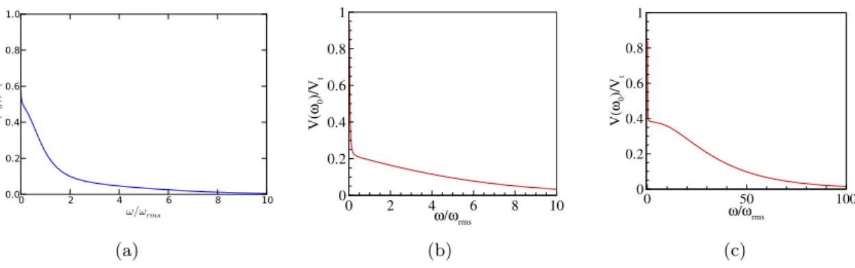
Figure 2: Volume of the region with vorticity magnitude greater than a given threshold ω > ω0, as
function of the vorticity magnitude threshold for the boundary layer (a), jet (b), and shear-free turbulence (c). ωrms is the reference rms vorticity used for each case, as described in section 2.
flows it has been observed that many statistics of the interface layer (e.g. conditional vorticity profiles in relation to the distance from the TNTI, the geometric shape of the TNTI) are weakly dependent of the particular value assumed by ω0 if it separates reasonably well the regions of turbulent and irrotational flow.
3.1. Detection of the turbulent/nonturbulent interface based on the volume of the turbulent region
In the present case the method described in Taveira et al. [9] is used to compute ω0. This method relies on the fact that the volume of the turbulent flow region, defined as the region where the vorticity magnitude is greater than a given threshold, exhibits a particular shape which is illustrated in figures 2(a), 2(b) and 2(c). The figures show the volume V of the turbulent region for the boundary layer, jet and shear-free turbulence cases, respectively, as function of the vorticity magnitude (threshold) used to detect it: V(ωI)i.e. we designate byωI
the particular value ofω0 obtained using thevolume method. As expected the turbulent volume is a monotonically decreasing function of the vorticity threshold, but in all three cases the rate of decrease changes with the vorticity magnitudeω. The turbulent volume falls sharply with the increase ofω until, for a givenω, the decrease rate slows down. For the jet case this happens at aroundω/ωrms≈0.3. It was observed that in practice any value ofω near this changing region
can be used to define the location of the TNTI. The particular value of the vorticity magnitude threshold used here ωI is defined as the inflection point of the turbulent volume
∂2
V(ω > ω0)
∂ω2 0
ω
0=ωI
= 0. (1)
3.2. Relation to other criteria for turbulent/non-turbulent interface detection
10-510-410-310-210-1 100 101 102 0.00 0.02 0.04 0.06 0.08 0.10 0.12 0.14 0.16 PDF Jet
10-710-610-510-410-310-210-1100101102 0.00 0.05 0.10 0.15 0.20 0.25 0.30
0.35 Boundary layer
10-4 10-3 10-2 10-1 100 101 102 ω/ωrms 0.00 0.01 0.02 0.03 0.04 0.05 0.06 PDF Isotropic
10-4 10-3 10-2 10-1 100 101 102 ω/ωrms 0.00 0.05 0.10 0.15 0.20 0.25 Channel
Figure 3: P.d.f. for vorticity magnitude
using ωrms as unit. The datasets
corresponding toChannelandIsotropic
correspond to a turbulent channel of size π × π/2 at Reτ = 950[29],
and a box of size 5123
at Reλ =
168[30] respectively. It is clear that fully turbulent flows present only one state, and the probability distribution of vorticity is unimodal.
If the flow is in two different states this scalar fieldφwill have a bimodal probability density function (p.d.f.). This means that most of the volume is either irrotational (φ≃0) or turbulent (φ≃1). It is reasonable to think that, if the turbulent/non-turbulent interface is a sharp front, its volume will be small. In consequence, if the interface has a characteristic value of φI, its
contribution to the p.d.f. will be small. Therefore, one can use the minimum between the two modes of the p.d.f. as a criterion to identify the threshold. This is a method to separate the two states of the flow on a practical way, more than a method to locate an interface. But, given the arbitrariness of the threshold definitions found in the literature, this one is particularly simple to apply.
While this method is used frequently in experiments, where seeding is a common practice, it is very difficult to implement in simulations. However, the vorticity magnitude can be used analogously to the concentration fraction φ. In external turbulent flows, the fluid is in two different states regarding vorticity, or in this case, vorticity magnitude. The probability distribution ofωhas a bimodal shape (figure 3), and a minimum that can be used as a practical criterion to obtain a thresholdωI.
This method is related to the volume filled by the fluid with vorticity from 0 toωI i.e. V(ωI),
that can be expressed from the p.d.f. of the vorticity magnitude, P(ω), as
V(ωI) =Vt
1−
Z ωI
0
P(ω) dω
, (2)
where Vt is the total volume of the domain. Differentiating twice this expression gives,
∂2
V(ωI)
∂ω2
I
=−Vt
∂P(ωI)
∂ωI
(3)
which shows that the minimum of the p.d.f. corresponds to an inflection point of the function
V(ωI) (figure 4), and gives the minimum-volume threshold.
10-7 10-6 10-5 10-4 10-3 10-2 10-1 100 101 102
0.0 0.2 0.4 0.6 0.8 1.0 1.2 1.4 1.6 1.8
Jet
Boundary Layer
10-7
10-6 10-5 10-4
10-3 10-2 10-1
100 101
102
ω/ω
rms0.0 0.2 0.4 0.6 0.8 1.0
V
(
ω
I)/V
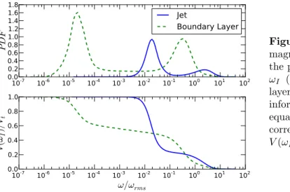
tFigure 4: P.d.f. for vorticity
magnitude (top) and volume covered by the points where vorticity is higher than
ωI (bottom) for a jet and a boundary
layer. The two curves contain the same information, since they are related by equation (3). Every extrema in P(ω) corresponds to an inflection point in
V(ωI)
two peaks are more separated than in the case of jets. However, it is difficult to predict their behaviour for higher Reynolds numbers, when vorticity has more time to decay and to adjust to the free stream.
3.3. Vorticity maps.
One goal of this work is to compare the differences and similarities between the TNTIs in boundary layers, jets and shear-free turbulence. A crucial issue is to define reference locations, within the TNTI, and reference vorticity values that allow such a comparison. The difficulty arises because of the different nature of the vorticity dynamics of these flows near the TNTI, despite vorticity being a small-scale quantity that should be ‘similar’ in all flows if the Reynolds number and associated separation of scales is large enough. However it is easy to understand that the particular vorticity dynamics is quite different in the flows analysed here because the vorticity generation takes place in different regions due to different mechanism in relation to the TNTI location. In shear-free turbulence, the vorticity is generated in the core of the turbulent region in much the same way as in isotropic turbulence, due to the interaction of existing fluctuating vorticity and fluctuating rate-of-strain, and is propagated without mean shear into the irrotational region across the TNTI. In the boundary layer, the wall, through the no-slip condition, provides most of the vorticity source which is then propagated away from the wall, eventually reaching the TNTI. The main source of vorticity in the boundary layer flow is therefore far from the TNTI location. Finally, in the case of the jet the situation is similar to the shear-free turbulence case, except that the vorticity propagates into the irrotational region across the TNTI under the influence of mean shear. Arguably, in high-Reynolds-number jets the generation of a small-scale dominated quantity such as vorticity is weakly dependent on mean shear effect, but this mean shear may indirectly influence the vorticity dynamics.
An interesting way to assess the vorticity in the three flows is to represent the p.d.f. of the vorticity magnitude for every point iny (where y is a distance in the flow to be defined latter). This generates a more complicated map, that encodes more information than the intermittency profile, but is harder to interpret. There are two characteristic regions, one with high vorticity and another one with low vorticity, separated by almost two orders of magnitude, and connected by the intermittent region. As will be shown below, this map allows us to give a more educated guess about what could be a consistent value for the threshold ωI to compare the three different
flow cases.
of the position (y - arbitrary units) across the intermittent region. The vorticity magnitude is normalised byωrms in the jet and in shear-free turbulence,ω∗=ω/ωrms, while in the boundary
layer it is normalised by a reference vorticity ωδ defined later in this section, ω∗ =ω/ωδ. Each
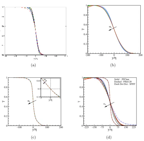
horizontal line in these graphs is a p.d.f. of vorticity magnitude at a given distance e.g. from the wall in the case of the boundary layer (Fig. 5(a)). Starting with the shear-free turbulence case (Fig. 5(c)) one can see that the shape of the p.d.f. clearly indicates the existence of two flow regions. For distances smaller than y/η ≈ 102 the p.d.f. of ω∗ exhibits the same shape, with the same peak at ω∗ ≈ 1.5, while for y/η ≥ 102
the p.d.f.s are quite different, with the peaks moving to smaller values of ω∗. The p.d.f. clearly illustrates the different behaviour of the turbulent and irrotational flow regions, with a nearly constant vorticity distribution in the turbulent region y/η ≤ 102
and much smaller vorticity peaks in the irrotational region
y/η >102, due to the negligible value of the vorticity magnitude there. The change observed for
y/η ≈102
is quite dramatic in that the peak values of the p.d.f. of ω∗ are discontinuous in the distance y, which is the consequence of a very sharp change of vorticity characteristics across the intermittent region. In the jet case (Fig. 5(b)) the p.d.f.s are similar, but the ‘change in character’ between the turbulent and irrotational regions seems to take place across a slightly bigger distance. Finally, for the boundary layer (Fig. 5(a)) one notices that the change between the turbulent and irrotational regions is less abrupt, lacking the discontinuity of the ω∗ peaks. Also, in this case, the range of values and ofω∗ seems to be larger than in the other cases and the peaks of the p.d.f.s of ω∗ change even within the turbulent region, because of the vorticity scaling laws near the wall.
In order to compare the characteristics of TNTIs of the three flows used here we need to choose a vorticity magnitude threshold ω0 allowing a meaningful comparison. To obtain this, figure 6(a) superimposes the above p.d.f.s in a single graph. The jet and shear-free turbulence compare well in this figure but the boundary layer presents difficulties due to the influence of the wall.
The dependence with y of the r.m.s. vorticity in boundary layers can be estimated if we assume that the energy production locally balances the dissipation, and use the logarithmic-layer scaling. Expressed in wall units, ǫ+
≈ ω+2
≈ ∂yU+ ≈ (κy+)−1, where κ is the von
K´arm´an constant. This suggests that
Ω+
(y) = (y+ )−1/2
(4)
can be used as a local surrogate for ωrms in the boundary layer, to compare it with the
free-shear flows. This rescaling is singular at the wall, but remains non-zero in the irrotational region, and provides a vorticity unit at the edge of the boundary layer, ωδ = hωiwallδ−
1/2 99 , which is useful in accounting for Reynolds-number effects in studying the TNTI. Figure 6(b) shows that normalizing the vorticity fluctuations with Ω(y) rescales the turbulent part of the p.d.f.s in the intermittency maps of the three flows to similar shapes.
By comparing the p.d.f.s in figure 6(b) we see that the change in the p.d.f. characteristics in the three flows takes place roughly at ω∗ ≈0.1. Therefore, in the following we will use,
ω0 = 0.1ωu (5)
as the threshold separating the turbulent from the nonturbulent regions in the three flows, where
ωu stands for the unit of vorticity used in each case: ωδ in boundary layers, and ωrms in jets
and shear-free flows.
4. Visualisation of the turbulent/nonturbulent interface
ω*
y/
η
-4.0 -3.0 -2.0 -1.0 0.0 0.5 1.0 1.5 2.0 2.5 10 10 10 10 10 10 10 10
10 10 10 10
(a)
ω*
y/
η
-2.0 -1.0 0.0 1.0
0.5 1.0 1.5 2.0 2.5 10 10 10 10 10 10
10 10 10 10
(b)
ω*
y/
η
-1.0 0.0 1.0 2.0
0.5 1.0 1.5 2.0 2.5 10 10 10 10 10 10
10 10 10
(c)
Figure 5: P.d.f.s of normalised vorticity
magnitudeω∗ as functions of the position
y across the TNTI. (a) boundary layer (vertical distance from the wall); (b) jet (distance from the jet centreline); (c) shear-free turbulence (distance from the centre of the turbulent region). The vorticity magnitude is normalised byωrms
in the jet and shear-free turbulenceω∗ =
ω/ωrms, and by the reference vorticityωδ
in the boundary layer ω∗ = ω/ω
δ. The
Kolmogorov micro-scale used in each flow is defined in section 2.
ω*
y/
η
-2.4 -1.6 -0.8 0.0 0.8 0.5
1.0 1.5 2.0 2.5
Solid : BL Dashed : PJChan
Dashed Dot : SFT
10 10 10 10 10 10 10
10 101010
10 10
10
10 -1.2 -0.2 0.8 2.3 2.4 (a) ω* y/ η
-2.4 -1.6 -0.8 0.0 0.8 1.0
1.5 2.0 2.5
Solid : BL Dashed : PJChan
Dashed Dot : SFT
10 10 10 10 10 10 10
10 101010
10 10
10 -1.2 -0.2 0.8 2.3
2.4
(b)
Figure 6: (a) Same as in figures 5(c), 5(b) and 5(a), but represented in the same graph using p.d.f.
(a) (b)
Figure 7: Iso-surfaces of vorticity magnitude corresponding to the TNTI in the boundary layer (a) and
jet (b) simulations. For the jet simulation the entire upper shear layer is displayed while only a fraction of the boundary layer is shown.
(a) (b)
Figure 8: Same as in figures 7(a) and 7(b) but showing only a piece of the TNTI. The lateral dimension
in both cases corresponds to roughly 1.5δ×1.5δ and 350η×350η (the Reynolds number based in the Taylor scale is similar in both flows).
of the interface location yi: in the boundary layer, red corresponds to smaller distances from
the wall, while in the jet it indicates higher distances from the jet centre.
The complexity of the TNTI can be appreciated in these figures. A large range of heights (yi) exists in both flows which clearly is not random. E.g., in the boundary layer regions of red
tend to be surrounded by regions of red also. The same happens in the jet case. In the jet, two large ranges of ‘hills’ seem to be separated by a long ridge, and are the imprint of the large-scale Kelvin–Helmholtz vortices of the jet underneath the TNTI.
5. Intermittency in boundary layers, jets and shear-free turbulence
The intermittent interaction between turbulent and irrotational fluid is a defining characteristic of free shear flows. But the concept of intermittency is qualitative. Jets, boundary layers, mixing layers and shear-free flows present a similar sharp interface, but how similar it is remains an open question.
The intermittency parameter γ, defined as the fraction of time that the flow surrounding a given point in space is turbulent, is the usual quantity to describe the intermittent properties of a flow. Its definition is surrogate to yet another variable, which is the criterion to separate between irrotational and turbulent states. Therefore, the intermittency parameter can be given a more precise definition that depends on the variable taken to quantify how turbulent the flow is, and a threshold. In this study, the vorticity magnitude is taken as a the base quantity, and the intermittency parameter is defined as the probability that the flow in a given point in space has vorticity higher than a threshold ω0,
γ =P(ω > ω0). (6)
A similar criterion can be used to detect the interface. Using the vorticity magnitude field, and the threshold ω0, we can assume that the isocontour ω(x, y, z) =ω0 is the outermost detection of the turbulent/non-turbulent interface.
The intermittency parameter is usually presented in the form of a profile that varies along the direction normal to the stream y. The intermittency profileγ(y) is linked to the detection criterion, because the probability to detect the interface at a given position of yi is
P(yi) =∂γ/∂y (7)
Figures 9(a), 9(b), and 9(c) show the intermittency factor for different values of the vorticity threshold for the boundary layer, jet and shear-free turbulence, respectively. Because for each value of ω0 the intermittency factor γ is centred at a different value of y, the curves were all shifted to have y= 0 whenever γ = 0.5, in order to allow the comparison between curves. The normal distance is normalised by the Kolmogorov micro-scale defined in section 2 for each flow. The intermittency factor is quite insensitive to the vorticity magnitude, particularly for the shear-free turbulence case. The three cases are compared in figure 9(d) where one can see thatγ
is very similar in the boundary layer and the jet, but definitively sharper in the shear-free case. In order to quantify these differences we define a macro and a micro intermittency scalesLγ
andlγ, respectively. Since the intermittency factor is function of the normal distance,γ =γ(y),
we define the coordinates corresponding to the start (ys) and end (ye) of the intermittency region
as γ(ys) = 1 andγ(ye) = 0 respectively. The macro intermittency scale is then defined as the
spatial extent of the intermittence region in the flow,
Lγ=|ys−ye|. (8)
The micro intermittency scale lγ is defined as the scale associated with the maximum local
derivative of the intermittency factor and thus represents the smallest length scale associated with the intermittency events,
lγ=|dγ/dy|−max1 . (9)
(a)
y/η
γ
-2000 -100 0 100 200 0.2
0.4 0.6 0.8 1
ω0
(b)
y/η
γ
-100 0 100 200
0 0.2 0.4 0.6 0.8 1
ω0 y/η
-5 0 5
0.35 0.5 0.65 ω0
(c)
y/d
a
-225 -150 -75 0 75 150 225
0 0.2 0.4 0.6 0.8 1
Solid : PJChan Dashed : PJkh120 Dash Dot Dot : SFIIT
t0
(d)
Figure 9: Intermittency parameter γin the three flows studied in the present work, as function of the
vorticity magnitudeω0. For each flow case y represents the normal flow direction, where the distance y was shifted so thatγ= 0.5 aty= 0 to allow the curves to be compared, and the distanceyis normalised by a characteristic Kolmogorov micro-scaleη, as discussed in section 2: (a) boundary layer; (b) jet and; (c) shear-free turbulence. (d) Comparison of the three flows: shear-free turbulence (dash-dot-dot), jet (solid blue line) and boundary layer (solid dark line). Other planar jet simulations are also added (e.g.
dashed line).
Figure 10: Definition of the macro intermittency
scaleLγ and micro intermittency scalelγ. Adapted
from La Rue and Libby [31].
Table 2: Macro intermittency scaleLγ and micro
intermittency scalelγ estimated for the three flows
analysed in the present work.
Flow Lγ/η lγ/η
Boundary layer 155 20 Turbulent jet 180 14
Shear-free 70 5
yI
0 0.05 0.1 0.15 0.2 0.25 0.3 0.35 0.4
0 2 4 6 8 10 12
1
1
2
2
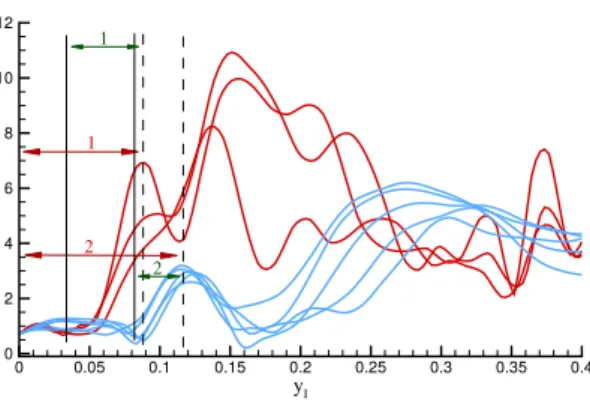
Figure 11: Sketch explaining the two methods
used to obtain the local values of δω. Method
1: Distance between the TNTI (yi = 0) and the
first ‘acceptable’ local vorticity maximum ωmax
(dashed). Method 2: Distance between the first ‘acceptable’ local maximumωmax(dashed) and the
previous local minimum (solid)
6. Statistics of the local interface thickness δω in the planar turbulent jet.
The mean interface thickness hδωi was analysed in turbulent planar jets and in shear-free
turbulence by da Silva and Taveira [14], for Reynolds numbers in 115 < Reλ < 160, where
it was defined by the length of the mean vorticity jump observed across the TNTI. In virtually all the flows assessed so far the conditional mean profile of ω exhibits a sharp jump at the TNTI and, after this jump, ω is roughly constant inside the turbulent region. Not surprisingly, da Silva and Taveira [14] observed that the large-scale eddy structure underneath the interface imposedhδωi. However no information exists for the local TNTI thickness. This information is
important in order to characterise the small-scale geometry of the interface and may be useful to develop detailed models of its local dynamics. The thickness we use here can be seen as a length scale associated with the process needed for the flow to go from the irrotational to the turbulent region. This is not a ‘geometrical’ thickness, which does not seem to exist. Rather it is a thickness associated with the dynamics of the vorticity near the TNTI.
In order to characterise the local interface geometry a local thicknessδω must be defined. In
the present work two definitions were used based on the local conditional vorticity profiles as shown in figure 11. With ‘method 1’ the local thickness δω is defined as the distance from the
location of the TNTI to the first ‘acceptable’ maximum, while in ‘method 2’, δω is defined as
the distance between this maximum and the nearest local minimum. The maximum vorticity observed in the conditional (instantaneous) profiles is ωmax.
6.1. Fractions of δω and ωmax from the total number of samples of both quantities
The tables 3 and 4 compile information from the local (instantaneous) values of the local interface thicknessδω and maximum vorticity at the interfaceωmax. The events are separated according
to the vorticity magnitude ωmax and the size of the vorticity jumpδω. Following Jim´enez and
Wray [30] we separate the vorticity events between intense vorticity (ωmax > ωivs, where ωivs
is the vorticity threshold that covers 1% of the total volume), weak (ωrms < ωmax < ωivs),
and background vorticity (ωmax < ωrms). It has been shown that regions of intense vorticity in
isotropic turbulence (intense vorticity structures - IVS) tend to be concentrated in thin vortex tubes (‘worms’), and that very few vortices exist with radius smaller than 3η or greater than 10η. We therefore separate the local TNTI thickness into incoherent (δω/η < 3), small scale
(3< δω/η <10), and intermediate-large scale (δω/η >10).
Table 3: Fraction of events contributing to the local TNTI thickness δω using ‘method 1’ (see text
for details). The events are separated according to the local vorticity magnitude into background, weak and intense events, and the local thickness is separated into δω/η >3, 3< δω/η <10, and δω/η > 10,
respectively.
Background Weak Intense
δω/η ωmax< ωrms ωrms< ωmax< ωivs ωmax> ωivs
Incoherent <3 4.7% 1.2% <0.1% 5.9%
Small scale >3 and<10 34.4% 35.5% 3.5% 73.4% Intermediate-large scale >10 6.9% 12.1% 1.5% 20.6%
Total 46.0% 12.1% 5.1% ≈100%
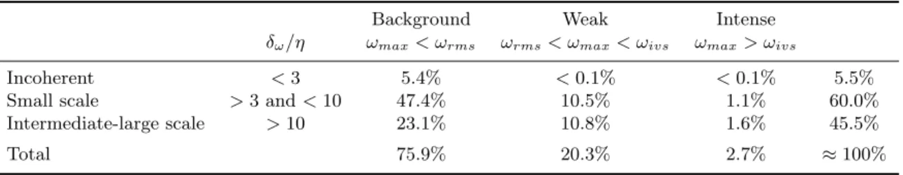
Table 4: As in table 3, using ‘method 2’ (see text for details).
Background Weak Intense
δω/η ωmax< ωrms ωrms< ωmax< ωivs ωmax> ωivs
Incoherent <3 5.4% <0.1% <0.1% 5.5%
Small scale >3 and<10 47.4% 10.5% 1.1% 60.0% Intermediate-large scale >10 23.1% 10.8% 1.6% 45.5%
Total 75.9% 20.3% 2.7% ≈100%
approximately 5% of the weak vorticity events are contained in vorticity jumps smaller than 3η, which suggests that no structures smaller than IVS exist near the TNTI. This result is consistent with da Silva et al. [15] where the tracking of the IVS near the TNTI was made, reaching similar conclusions. On the other hand most of the observed events are associated with small scale thickness (3< δω/η <10) and weak and background vorticity. This is an interesting result
because the mean vorticity thickness for this simulation is slightly higher hδωi/η ∼ 16η ∼ λ.
However very few of the events are associated with particularly strong vorticity magnitudes, again consistent with da Silva et al. [15]. This suggests that the TNTI is mostly ‘made up’ of small-scale eddies but exhibiting vorticity magnitudes that are smaller than the IVS from the core of the turbulent region. This also shows, as expected, that the vorticity magnitude at the TNTI is very small consisting in mostly background and some weak vorticity.
6.2. Probability density functions of local interface thickness
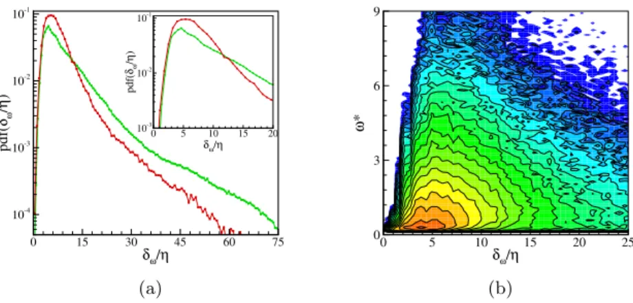
Figure 12(a) shows p.d.f.s of local interface thickness δω computed with the two methods
described before. The p.d.f. shows that δω displays a large range of values with a peak around
δω/η ≈ 5−6 which coincides with the mean radius of the IVS, while the mean thickness
-aroundδω/η ≈16 in this case - is not far off, but results from averaging a large range of possible
values, and does not arise ‘naturally’ from the data. Arguably the scatter in the results will be even higher at high Reynolds numbers, where no large-scale eddy is likely to survive the background field of fluctuating strain, implying that the mean value of δω will probably tend
more to hδωi ∼η than tohδωi ∼λas is the case here.
Figure 12(b) shows the joint p.d.f. of the local vorticity maximum ωmax and of the TNTI
thicknessδω. It is difficult to observe a correlation between the two quantities, which agrees with
δω/η
pdf(
δω
/
η
)
0 15 30 45 60 75
10-4
10-3
10-2
10-1
δω/η
pdf(
δω
/
η
)
0 5 10 15 20 10-3
10-2
10-1
(a)
δω/η
ω
*
0 5 10 15 20 25
0 3 6 9
(b)
Figure 12: (a) P.d.f.s of local thickness δω from the instantaneous vorticity conditional profiles for
the planar jet using ‘method 1’ (green) and ‘method 2’; (b) Joint p.d.f.s of vorticity magnitudes
ω∗ = ω
max/ωrms and local thickness δω from the instantaneous vorticity conditional profiles using
‘method 1’.
7. Low vorticity regions embedded in turbulent flow, and their role in entrainment.
One resilient discussion about the mechanism of entrainment is how the irrotational fluid actually acquires vorticity. Two different possibilities can be found in the literature: one in which vorticity is transmitted by direct shearing contact with the turbulent eddies across the turbulent/non-turbulent interface, and a second in which some coherent structure encloses the irrotational flow forming pockets or bubbles (defined as regions of low vorticity completely surrounded by fluid at higher vorticity) that are later given vorticity. The two mechanisms are usually called nibbling and engulfing respectively. This distinction is ambiguous. A pocket can be considered a sign of nibbling and engulfment. To avoid this ambiguity, engulfment will be considered only if the zone with low vorticity is completely surrounded, and becomes isolated.
Nibbling is inherently small-scale, because direct shearing contact can only happen by effect of viscosity. Engulfment, however, can happen at many different scales. Low-vorticity bubbles are as large as the coherent structure that encloses them, which includes almost any scale present in the flow. It is also a purely three-dimensional definition, and cannot be applied if vorticity is measured on a plane, or the data set provides only one vorticity component. Fortunately, the data available for this study fulfils the previous requirements, and algorithms for fast identification of isolated structures (commonly called labeling) are presently available.
Figure 13 is the result of labelling two different flows with two different thresholds, below and above the proposed value to detect the turbulent/non-turbulent interface for the jet
ω0 = 0.1ωrms. A cut of the contour of every structure detected is marked with a solid line. It can be seen in figure 13b, that the flow of the jet sparsely marked with many low-vorticity regions. At this low threshold, the question arises whether these regions are a product of the interaction between the turbulent eddies and the free stream, or a feature of any turbulent flow. To find an answer to the previous question, the planar jet is compared to a homogeneous and isotropic turbulence (HIT) box at a similar Reynolds number (Reλ = 168)[30], where the
isolated bubbles have been detected using the same technique and a comparable threshold. Given that HIT contains no such thing as a turbulent/non-turbulent interface, any obvious difference between the two flows may be due to the interaction between the turbulent eddies and the free stream.
Figure 13: Cuts of the boundaries of low-vorticity bubbles at different thresholds for jets and HIT. The lengths are represented in the Kolmogorov units. Given that the outer stream is identified as a low-vorticity spot, the interface detection can always be seen in the case of the jet. In the case of the higher threshold in homogeneous turbulence, there is a single low-vorticity region that covers a relevant part of the volume, and is also detected as a spot.
and a second one at a higher threshold (figure 13 c, and d). If one ignores that the bubbles in the planar jet are confined to the fully turbulent flow, the shape and density of bubbles is pretty similar. But this observation, based purely on perception, is not quantitative.
To add more consistency to the previous comparison, the probability density of the volumes of these bubbles is computed at four different thresholds, for the planar jet and the HIT box. The context of those thresholds is clarified by the figure 14, where every threshold is marked with a vertical dashed line. The values cover a range of values of half an order of magnitude, close to the one chosen to detect the interface. The same unit for vorticity is used in both flows given that, according to figure 14,ωrms makes the two flows comparable in the explored range.
The p.d.f of the size of the low-vorticity bubbles, expressed as the cubic root of their volume, is presented in figures 15(a-d). It follows a power-law distribution with an exponent of −3, represented in figure 15(a-d) as a dashed line, which argues for a self-similar origin without a characteristic length scale.
Interestingly, figure 15 shows that the HIT and planar jets follow a similar power law for bubble size, strongly suggesting that their formation is not heavily affected by the presence of irrotational flow in the case of the jet.
10-5 10-4 10-3 10-2 10-1 100 101 ω/ωrms 10-6 10-5 10-4 10-3 10-2 10-1 100 101 PDF Jet HIT
Figure 14: Probability density of vorticity
mag-nitude for planar jets (solid line) and homogeneous isotropic turbulence (circles) using the r.m.s. of vor-ticity magnitude as unit. The bimodal behaviour in jets is described in figure 3. The distribution of vorticity in the peak corresponding to the fully tur-bulent fluid is similar, and confirms that ωrms is a
suitable unit to compare HIT and planar jets. The four vertical dashed lines correspond to the thresh-olds used in the results presented in figure 15
100 101 102 103
10-4 10-3 10-2 10-1 100 101 PDF
(a)ω/ωrms=0.08 Jet HIT
100 101 102 103
10-4
10-3
10-2
10-1
100
101 (b)ω/ωrms=0.14
100 101
102 103
3 p V/η 10-4 10-3 10-2 10-1 100 101 PDF
(c)ω/ωrms=0.23
100 101
102 103
3 p V/η 10-4 10-3 10-2 10-1 100
101 (d)ω/ωrms=0.40
Figure 15: Probability density of the
characteristic length of the low-vorticity bubbles for homogeneous isotropic tur-bulence (circles) and planar jets (solid lines). The thresholds are represented in figure 14 as dashed lines. The straight lines correspond to the exponent for scale invariance (√3
V /η)−3 .
low vorticity are found in the fully turbulent fluid, but they are very similar to the bubbles found in internal flows, where the mentioned mechanism cannot occur.
8. Conclusions
Direct numerical simulations of a boundary layer, a planar jet and shear-free turbulence at Reynolds numbers slightly higher thanReλ = 100 are used to compare the characteristics of the
TNTI in different flows.
A prerequisite to compare the three TNTI is the determination of the location of the TNTI in each flow. In the present work, the technique used for this detection relies on computing the volume of turbulent region as a function of the vorticity magnitude. For the three flows analysed here, the volume of the turbulence region exhibits a characteristic change with the vorticity magnitude, displaying an inflection point. The vorticity magnitude threshold corresponding to this inflection point is used to define the TNTI. It is shown that this method is equivalent to well-known experimental methods used to detect scalar interfaces.
Visualisations of the TNTIs for boundary layers and jets are compared, and show that the statistics of the interface height are not random and the observed differences suggest the imprint of the different underlying large-scale vortices in the two flows.
The intermittency parameters were computed for the three TNTIs, and length scales were defined. A large scale associated with the maximum extent of the intermittency region and a small scale associated with the strongest gradient across this region. In the present case the large-scale intermittency regions for boundary layers and jets were comparable and significantly larger than in the shear-free case. Interestingly the small intermittency scale is similar to the computed vorticity thickness (or jump) observed in the jet and shear-free case, suggesting another method to quantify the so called TNTI thickness (identified) as the turbulent sub-layer.
Finally, an analysis is made of the irrotational bubbles trapped inside the turbulent region, which are typically associated with ‘engulfing’ events in several flows. The analysis shows that, contrary to the classical view, the spots of low vorticity found inside the jet follow a power law, which is exactly the same observed in isotropic turbulence, where engulfing events do not exist. This suggests that the vast majority of these regions are not associated with engulfment.
Acknowledgments
This work was performed in part during the first Multiflow summer school at Madrid, and partially funded by the European Research Council.
References
[1] Corrsin S and Kistler A L 1955Free-stream Boundaries of Turbulent FlowsTech. Rep. TN-1244 NACA [2] Townsend A A 1966 The mechanism of entrainment in free turbulent flowsJ. Fluid Mech.26689–715 [3] Mathew J and Basu A 2002 Some characteristics of entrainment at a cylindrical turbulent boundaryPhys.
Fluids 142065–72
[4] Westerweel J, Fukushima C, Pedersen J M and Hunt J C R 2005 Mechanics of the turbulent-nonturbulent interface of a jetPhys. Rev. Lett.95174501
[5] Westerweel J, Fukushima C, Pedersen J M and Hunt J C R 2009 Momentum and scalar transport at the turbulent/non-turbulent interface of a jetJ. Fluid Mech.631199–230
[6] Holzner M, Liberzon A, Nikitin N, L¨uthi B, Kinzelbach W and Tsinober A 2008 A Lagrangian investigation of the small-scale features of turbulent entrainment through particle tracking and direct numerical simulation
J. Fluid Mech.598465–75
[7] da Silva C B and Pereira J C F 2008 Invariants of the velocity-gradient, rate-of-strain, and rate-of-rotation tensors across the turbulent/nonturbulent interface in jetsPhys. Fluids 20055101
[8] Taveira R R and da Silva C B 2013 Kinetic energy budgets near the turbulent/nonturbulent interface in
jetsPhys. Fluids25015114
[9] Taveira R R, Diogo J S, Lopes D C and da Silva C B 2013 Lagrangian statistics across the turbulent-nonturbulent interface in a turbulent plane jetPhys. Rev. E 88043001
[10] Townsend A A 1976The Structure of Turbulent Shear Flow (Cambridge: Cambridge University Press) [11] Gampert M, Narayanaswamy V, Schaefer P and Peters N 2013 Conditional statistics of the
turbulent/non-turbulent interface in a jet flowJ. Fluid Mech.731615–38
[12] Wolf M, Luthi B, Holzner M, Krug D, Kinzelbach W and Tsinober A 2013 Investigations on the local entrainment velocity in a turbulent jetPhy. Fluids 24105110
[13] da Silva C B and dos Reis R J N 2011 The role of coherent vortices near the turbulent/non-turbulent interface in a planar jetPhil. Trans. R. Soc. A369738–53
[14] da Silva C B and Taveira R R 2010 The thickness of the turbulent/nonturbulent interface is equal to the radius of the large vorticity structures near the edge of the shear layerPhys. Fluids 22121702
[15] da Silva C B, dos Reis R J N and Pereira J C F 2011 The intense vorticity structures near the turbulent/non-turbulent interface in a jetJ. Fluid Mech.685165–90
[16] Mandelbrot B B 1982The Fractal Geometry of Nature(New York: W. H. Freeman)
[17] Sreenivasan K R 1991 Fractals and multifractals in fluid turbulenceAnn. Rev. Fluid Mech.23539–600 [18] Frederiksen R D, Dahm W J A and Dowling D R 1997 Experimental assessment of fractal scale similarity
in turbulent flows. Part 3. Multifractal scalingJ. Fluid Mech.338127–55
[20] de Silva C M, Philip J, Chauhan K, Meneveau C and Marusic I 2013 Multiscale geometry and scaling of the turbulent-nonturbulent interface in high Reynolds number boundary layersPhys. Rev. Lett.111044501 [21] Westerweel J, Hofmann T, Fukushima C and Hunt J C R 2002 The turbulent/non-turbulent interface at
the outer boundary of a self-similar turbulent jetExp. Fluids33873–78
[22] Simens M P, Jim´enez J, Hoyas S and Mizuno Y 2009 A high-resolution code for turbulent boundary layers
J. Comput. Phys.2284218–31
[23] Borrell G, Sillero J A and Jim´enez J 2013 A code for direct numerical simulation of turbulent boundary layers at high Reynolds numbers in BG/P supercomputersComput. Fluids 8037–43
[24] Sillero J A, Jim´enez J and Moser R D 2013 One point statistics for turbulent wall-bounded flows at Reynolds numbers up toδ+
= 2000Phys. Fluids 25, 105102
[25] Perot B and Moin P 1995 Shear-free turbulent boundary layers. Part 1. Physical insights into near-wall turbulenceJ. Fluid Mech.295199–227
[26] Teixeira M and da Silva C B 2012 Turbulence dynamics near a turbulent/non-turbulent interface J. Fluid
Mech.695257–287
[27] Bisset D K, Hunt J C R and Rogers M M 2002 The turbulent/non-turbulent interface bounding a far wake
J. Fluid Mech.451383–410
[28] Prasad R and Sreenivasan K R 1989 Scalar interfaces in digital images of turbulent flows Exp. Fluids 7 259–264
[29] Lozano-Dur´an A and Jim´enez J 2014 Effect of the computational domain in direct simulations of turbulent channels up toReτ= 4200Phys. Fluids 26011702
[30] Jim´enez J, Wray A A, Saffman P G and Rogallo R S 1993 The structure of intense vorticity in isotropic turbulenceJ. Fluid Mech.25565–90