A Computational Method for
Finding All the Roots of a Vector Function
Pedro J. Zufiria and Ramesh S. GuttaluABSTRACT
Based on dynamical systems theory, a computational method is proposed to locate all the roots of a nonlinear vector function. The computational approach utilizes the cell-mapping method. This method relies on discretization of the state space and is a convenient and powerful numerical tool for analyzing the global behavior of nonlinear systems. Our study shows that it is efficient and effective for determining roots because it minimizes and simplifies computations of system trajectories. Since the roots are asymptotically stable equilibrium points of the autonomous dynamical system, it also provides the domains of attraction associated with each root. Other numerical techniques based on iterative and nomotopic methods can make use of these domains to choose appropriate initial guesses. Singular manifolds play an important role in limiting the extent of these domains of attraction. Both a theoretical basis and a computational algorithm for locating the singular manifolds are also provided. They make use of similar state-space discretization frameworks. Examples are given to illustrate the computational approaches. It is demonstrated that for one of the examples (a mechanical system), the method yields many more solutions than those previously reported.
1. I N T R O D U C T I O N
In this paper, we consider the problem of finding all the solutions to the nonlinear vector algebraic equation
nonlin-early coupled. The problem of determination of the roots or zeros of a system of nonlinear algebraic equations is often encountered in science and engineer-ing, especially when dealing with nonlinear phenomena. The same problem is posed when looking for periodic solutions of nonlinear differential equations and fixed points of maps. One notes that, in general, Equation (1) may possess more than one root, and two questions often arise when dealing with it. The first question is concerned with how to obtain just any one solution of (1). The second question refers to locating all the solutions. This paper primarily focuses on the second question, which has significant bearing on the first question. A theory for locating all the zeros of (1) has been proposed by Zufiria and Guttalu [30], and is based on a dynamical system approach. Computational aspects of finding all zeros will be treated in this paper by making use of the theory developed there.
There exists an extensive literature dealing with both theoretical and computational aspects of obtaining a solution to (1). We give only a brief account of it here. Iterative techniques, usually based on the contraction-mapping theorem (see Marsden [23]), are a notable class of such methods. The literature is vast on the analysis of local convergence properties of various iterative procedures; for details refer to Ortega [25], Ostrowski [28], and Rheinboldt [29]. In general, all the iterative techniques require the initial guess to be inside a regular neighborhood (radius of convergence) of the root. Results given by Axelsson [1], Brent [3], Garcia and Zangwill [7], Griewank and Osborne [9], Hirsch and Smale [13], Ortega [26], and Rheinboldt [29] guarantee convergence to a single root when the initial guess falls in a prescribed region. Newton-like methods are the most popular among the iterative techniques and are routinely employed to obtain a root of (1). It is well known that it is not always possible to find all the roots of / by these methods alone.
Another class of methods to determine the roots are numerical techniques based on the continuation or homotopy ideas; see Garcia and Zangwill [7], Morgan [24], and Ortega and Rheinboldt [27]. When the vector field / is a polynomial, it is known that one can obtain all the roots, both real and complex (see Morgan [24]). Even though homotopic ideas are very powerful, unfortunately they do not always yield the location of all the roots when f{x) is a general function of x.
equivalently the topological degree of a map), has been developed by Hsu and Guttalu [17] and by Hsu and Zhu [18] for locating all the roots of / . The method presented in this paper differs from the index-theory approach with its emphasis on dynamical system formulation. Besides yielding all the solutions, our approach, based on the cell-mapping method, provides addi-tional information useful in conjunction with iterative and homotopic tech-niques.
In this paper we make use of a certain autonomous dynamical system to help locate the roots of the vector function / . The dynamical system is such that its equilibrium points are the roots of / , which are guaranteed to be asymptotically stable. This implies that there exist trajectories in the state space which approach these equilibrium solutions asymptotically. A detailed stability analysis of the autonomous dynamical system together with an estimation of the regions of attraction of each root of / can be found in Zufiria and Guttalu [30]. Manifolds where the gradient of / is singular have been identified as playing a significant role in influencing the global behavior of the dynamical system as well as in delineating the regions of attraction.
In order to locate computationally the zeros of the nonlinear vector function / , we will employ the dynamical system studied by Zufiria and Guttalu [30] in conjunction with the simple cell-mapping technique described by Hsu [19]. The method of cell mapping exploits the idea of discretization of space and avoids repetitive, time consuming calculation of trajectories of dynamical systems. It is capable of locating stable solutions of strongly nonlinear systems. Also, the method is computationally well suited for deter-mining the global behavior of nonlinear systems. Hence, the cell-mapping technique is an efficient and powerful computational tool in our case, not only for locating all the zeros of / , but also for delineating the regions of attraction associated with each of them. The number of roots determined by the approach given in this paper depends on the extent of the state space discretized and the fineness of discretization as determined by the cell size. As is characteristic of any finite-precision calculation, roots extremely close to each other can only be located by reducing the cell size.
In the same spirit, based on the discretization of state space, a novel approach for locating the singular manifolds is developed here. A few analytical results are established to support the validity of the computational algorithm that is presented. The algorithm is in general capable of solving for zeros of any scalar function of several variables.
applicable to dynamical systems, other than the one studied by Zufiria and Guttalu [30], which can be constructed to help locate the roots of / .
The rest of the paper is organized as follows. In Section 2, the dynamical system employed for the purpose of locating zeros of / is given, followed by a summary of appropriate results taken from Zufiria and Guttalu [30]. In Section 3, a cell-mapping formulation of the dynamical system is provided for numerical root determination as well as for computing the domain of attrac-tion associated with each root. Theoretical results and a computaattrac-tional algorithm for locating the singular manifolds are given in Section 4. Section 5 provides a brief summary of the numerical aspects associated with the implementation of the method of finding zeros. Computational results for a variety of examples are given in Section 6. This section includes the problem of locating the fixed points of a map which represents an impulsive, periodic, parametrically excited, two-degree-of-freedom mechanical system. For this problem, many more solutions are discovered by using the method outlined in this paper than were obtained by Hsu and Guttalu [17] employing index theory. Concluding remarks appear in Section 7.
2. FORMULATION OF AN AUTONOMOUS DYNAMICAL SYSTEM
A key idea in finding the zeros of / is to relate this problem to the problem of determination of equilibrium points of an appropriate dynamical system. Then one can make use of the rich mathematical theory available to deal with dynamical systems arising from such a study. Trajectories of the related dynamical system can provide useful information about the location of zeros of / . A great variety of dynamical systems may be formulated to help locate the zeros of / . We will focus primarily on a continuous-time dynamical system associated with the system of algebraic equations (1). This au-tonomous dynamical system has been studied in Zufiria and Guttalu [30] and is given by
i(t)-F{x)--r\x)f(x), F:RN^W, (2)
later. For a proof of the results stated in this section and other related topics, the reader is referred to Zufiria and Guttalu [30].
2.1. Relation to Homotopic Methods
Dynamical systems of the type described by (2) are extensively employed by homotopic techniques in an implicit manner to find zeros of the vector function / ; see Garcia and Zangwill [7], Gladwell [8], Hirsch and Smale [13], and Keller [20]. Assume that x in (1) depends on a parameter t. Taking derivative of f(x) with respect to t, we have
A*)=Vxf(x)x
= -J(x)r\x)f(x)
= - / ( * ) , (3)
where we have made use of (2). On integration, (3) yields the solution
/ ( x ( í ) ) = / ( x0)e í° -í, x0 = x{t0), t0G R . (4)
It is clear from (4) why one often defines the homotopy function
h(x)=f(x)-f(x0)e'o-' = 0, t>t0. (5)
By differentiating (5) once with respect to t, the differential equation (2) is readily obtained if the matrix J(x) is nonsingular. If a solution x(t) of the differential equation (2) exists for all t > t0, then it is known from Equation
(5) that this solution approaches a root of / a s t -> oo. Assuming that / is nonsingular, convergence theorems are provided and a number of algorithms are proposed for finding zeros in the abovementioned references. The essen-tial aim there is to follow paths that lead to a single solution of (5) and hence to a root of / .
To gain further insights into the behavior of the dynamical system (2), consider the inverse problem of determining f(x) when the vector field F(x) of (2) is given. In this case, / is determined by N first-order, decoupled linear homogeneous partial differential equations given by
£ dfi
fi(xl,...,xN)=- £ —F,, ¿ = 1,2,....N, (6)
where df/dxj are the components of the matrix J(x). By considering time t as a parameter, a solution of (6) can be sought using the method of characteristics (see Carrier and Pearson [6]) to obtain
x = F(x), x^RN, (7)
f,= -ft, ¿ = 1,2,...,AT. (8)
Whereas the parametric evolution of the state-space vector x(t) [the un-known vector in (1)] given by (7) is the same as that of the original dynamical system (2), the time evolution of the vector f(x(t)) given by (8) is identical to Equation (3) obtained by taking the time derivative of / . The equations (8) assume a solution of the form fi(t) = fix^e'0"*, meaning that as i-»oo,
fi(t)-*0. However, the path x(t) along which a zero of / is approached is governed by the dynamical system (7). These results are identical to those previously obtained by considering the homotopic method. Even though Equation (8) says that / - » 0 as f —> oo, it does not necessarily imply that the time evolution of the unknown x(t) governed by (7) approaches a constant vector. In general, the dynamical system (7), which is identical to (2), can display very complicated trajectory behavior. It is well known that, for some specific forms of F, initial states may lead to chaotic trajectories (for example a Lorenz attractor; see Guckenheimer and Holmes [10] and Hsu [19]).
Since complicated dynamic behavior is possible with (2), homotopic methods impose restrictions on / in (2) in order to generate smooth paths which lead to a single solution. The computational method to be presented later is applicable to (2) with no restrictions on /, and it has the potential of locating roots which may not be found with homotopic methods. The method is also capable of locating all the roots at once, the only limitation being that imposed by the level of discretization.
2.2. Relationship between the Zeros of f and F
The Jacobian matrix / is called regular at x e R " if det J(x)¥=0; other-wise it is called singular, or irregular, at x. Let x* e R^ denote a root of / , i.e., f(x*) = 0. Then, similar definitions apply to regular and singular roots of/.
In Zufiria and Guttalu [30], a detailed study has been made on how the vector field F = — J~lfoi (2) brings out features of the system dynamics not
where / is singular. However, singularity of / at a point does not imply that F is undefined at that point. Furthermore, the following lemmas proved in Zufiria and Guttalu [30] are provided here to indicate the relationship between the regularity of / and the vector field F.
LEMMA 1.
(a) F(xd) is defined if and only iff(xd) belongs to the image ofJ(xd).
(b) Let F(xu), xu e RN, be undefined. Then J(xu) is singular.
Note that in some cases F(xd) could be defined but not uniquely. In this
case, sometimes it is possible to choose a value of F(xd) that preserves the
continuity of F at that point. If this happens, then we will consider that the function F( •) is defined at such a point.
LEMMA 2. Suppose that J(x*), x* e R^, is nonsingular. Then f(x*) = 0 if and only if F(x*) = 0. In other words, x* is an equilibrium point of (2).
LEMMA 3. Let F(x*) = 0, x* e R^. Then f(x*) = 0.
LEMMA 4. F(x0), x0 e R^, is defined if and only if F is continuous at
x = x0.
2.3. Asymptotic Stability and Domains of Attraction of Zeros
In this subsection, we highlight certain local and global stability properties of the dynamical system (2) by stating results without proof. Asymptotic stability of all the equilibrium points of the system (2) is established in the following theorem.
THEOREM 1. Suppose that J is regular and VXJ 1 is defined at a zero x*
off. Then x* is an asymptotically stable equilibrium point of (2).
THEOREM 2. Given f, consider the scalar function
V ( x ) = /r( z ) / ( x ) = / ( x ) - / ( x ) , V : R " - R , (9)
where fT(x) is the transpose off(x). Suppose that F(x*) = 0, x* e R^, that
is, x* is an equilibrium point of (2). Then V is a strict Lyapunov function of (2) for x*.
THEOREM 3. Let x* be a zero of f. If F(x*) = 0, then x* is an asymptotically stable equilibrium point of (2).
The strict Lyapunov function V(x) is capable of providing estimates of the regions of initial states such that trajectories starting there are asymptotically attracted to the equilibrium points of the system (2). Thus, V(x) provides an estimate of the region of initial guess which when used with iterative techniques may converge to a zero of / . To elaborate on this, we define domain of attraction as follows.
DEFINITION 1. The domain of attraction (or region of attraction) Dx» of
an asymptotically stable equilibrium point x* of the system (2) is given by the set
D , . = { x ( i o ) | | | x ( 0 - x * | | - » 0 a s t - » o o } (10)
for i0 > 0. For the autonomous system (2), t0 is arbitrary.
The boundary of the level curves V(x) = I, for appropriate constant I and for a given zero x* of / , defines a region 4r. This region ¥ is a subset of Dx,,
such that any initial state in ¥ will asymptotically approach the equilibrium point x*. The result is stated in the following theorem.
THEOREM 4. Let ^ = {x\V(x)<l} be a bounded region with the boundary d^ on which V(x) = 1, / e R+. Suppose that ty contains only one root x* of f. If F is defined in ty, then ¥ is included in the domain of attraction Dx» associated with x* of (2).
way in which system trajectories evolve in the state space. In the case when / has only isolated roots, the behavior of trajectories of the system is provided in the following theorem.
THEOREM 5. Suppose that f has only isolated zeros. Then every trajectory of the dynamical system (2) can only have one of the following behaviors:
I. ||*(f )|| ~~* °° °* H T e R+. ( / / T is finite we have a finite escape time; see LaSalle and Lefschetz [21]).
II. x(t)->xs as t->T, where F(xs) is not defined and x(t) is not defined for t >T.
III. x(t) -> x* as t -»oo, where F(x*) = 0 (that is, x* is a root off).
In order to understand the global behavior of the dynamical system (2) in a more general manner, we make use of the concepts of directionally defined vector field, singular manifolds, barrier manifolds, and isolated regions.
DEFINITION 2. F(x) is directionally defined at x = x0 if there exists a
sequence of points xk approaching x0 such that lim^ — xF(xk) is defined.
DEFINITION 3. F(x) is directionally undefined at x = x0 if it is not
directionally defined.
We note that when F(x) is directionally undefined at x = x0, then
1
lim ••-,, . , , = 0 , (11) *-*« | | F ( * ) | |
where ||-|| is any norm in R^.
DEFINITION 4. A singular manifold S¡, ¿ = 1,2,..., is defined as an (N — l)-dimensional manifold
DEFINITION 5. Let x¡ and x2 be any two points on either side of a
singular manifold S¡. A barrier manifold B¡, i = 1,2,..., is defined as a singular manifold for which any pair of directional limits satisfy
lim [ n - F ( x1) ] [ n - F ( *2) ] < 0 (13)
x¡,x2-*xB
or at least one of the conditions
lim F(x1) = 0, lim F ( x2) = 0, (14)
xl ~ * XB x2~* XB
where n is a vector normal to the manifold B¡ at x = xB, xB e B{.
This means that each B¡ belongs to the set of connected (N—l)-dimensional manifolds where the matrix / is singular. A dynamical system of the type (2) may possess several barrier manifolds. It should be noted that, in general, the problem of locating the singular manifolds may be as difficult as finding the zeros of / .
DEFINITION 6. An isolated region £2¡ c R^, i = 1,2,..., is any region in which
1. Í2, is connected;
2. i 2 , n B . = 0 , j = 1,2,...;
3. 5Í2¡ c U ¡ B , where díl¡ is the boundary of 2r
The isolated regions are the regions separated by the barrier manifolds. An important question arises as to the number of roots of / that exist in fi, and how domains of attraction are related to them. The following results relate the barrier manifolds, isolated regions, and domains of attraction.
COROLLARY 1. Let £2 be an isolated region. Then the dynamical system (2) does not have any equilibrium point in ü¡ other than the zeros x* of f for ¿ = 1,2,....
THEOREM 7. Let x* be a zero of f such that F(x*) = 0. If Dx, is the
domain of attraction associated with x* of the dynamical system (2), then Dl t c Í1 for some specific j .
THEOREM 8. Suppose that J is regular in an isolated region fi ..
(a) Consider the case N—l, I G R . Then S2, contains at most one asymptotically stable equilibrium point x* of the system (2) (with the corresponding domain of attraction given by Dxj,).
(b) Consider the case N^2, x e RN. Then it is possible that Qj contains more than one asymptotically stable equilibrium points x* of (2), k = 1,2,... (with their donuiins of attraction Dx„).
The above definitions have been useful in establishing certain key results regarding the global behavior of the dynamical system (2). These results indicate how isolated regions bound and restrict the extent of the domains of attraction associated with the zeros of / . An estimate of the sizes of domains of attraction is provided by the Lyapunov function V(x). In order to obtain domains of attraction completely (at least from a numerical standpoint), one resorts to global computational analysis. The method of cell mapping is one such powerful technique which can efficiently provide results in this case.
3. CELL-MAPPING FORMULATION
In this section, we discuss the general computational cell-mapping tech-nique based on discretization of the state space which can be used for global analysis of general nonlinear dynamical systems.
3.1. A Brief Review of Cell Mapping
In order to construct a cellularly structured state space S, let the coordi-nate axes of the state variable components x¡, i = 1,..., N, be divided into a large number of intervals of uniform size ht. The new state variable z¡ along
the x(-axis is defined to contain all x, such that
(*
<-¿K<*
1<U + Í)V (15)
By definition, z¡ in (15) is an integer. A cell vector z is defined to be an iV-tuple z¡, i = l,...,N. Clearly, a point x e R^ with components xi belongs
to a cell Z&.S with components z¡ if and only if xi and z¡ satisfy (15) for all
t. The space S consisting of elements which are Af-tuples of integers is referred to as an N-dimensional cell space. If 2VC denotes the number of intervals along the xraxis, then the cell space S contains a total of Nc X Nc
X • • • X N cells.
In the cell state space S, one can define a cell-to-cell mapping dynamical system in the form
z ( n + l ) = C ( z ( n ) ) , C : S - » S , n € Z , (16)
where C is referred to as a simple cell mapping and is conceived of as a mapping from a set of integers to a set of integers. Equation (16) then describes the evolution of a cell dynamical system in AT-dimensional cell state space S. For a detailed treatment concerning the properties of the map C and its refinements, the reader is referred to the research monograph by Hsu [19]. In the following sections, we concentrate on simple cell mapping only and refer to it simply as cell mapping.
3.2. Periodic Motion
The dynamics of the cell mapping system (16) is characterized by singular cells consisting of equilibrium cells and periodic cells. An equilibrium cell z* is given by z* = C(z*). A periodic cell of period K G Z+ (or simply a P-K cell) is a set of K distinct cells {z*(k)\k = 1,2,..., K) such that
z*(fc + l ) = C * ( z * ( l ) ) , fc = l , 2 , . . . , K - l ,
(17) z*(l) = C * ( z * ( l ) ) ,
where C* means the mapping C applied k times. This set is said to constitute a periodic motion of period K, or simply a F-K motion. An equilibrium cell in this context is a P-l cell. A regular cell is one which is not singular.
contiguous cells are equilibrium cells. An equilibrium cell, when not isolated, may have several contiguous equilibrium cells. Then, a complete set of contiguous equilibrium cells is referred to as a core of equilibrium cells. The size of the core is determined by the number of cells in it. Similar definitions apply to periodic cells.
3.3. Creating a Cell Mapping from an Autonomous Dynamical System To obtain a cell mapping associated with the autonomous dynamical system (2), the following procedure may be employed. First, construct a cell space structure in the state-space region with cell size hi in the x ¡-direction.
Let xd(t0) denote the center point of the cell z(t0), so that xf(t0) = fyz^t,,).
Integrate the state equations (2) from time t = t0 to time t = tQ + T, where T
is the integration time step size. Suppose that the trajectory starting from xd(t0) terminates at xd(t0 + T). The cell in which x\t0 + T) lies is taken to
be z(t0 + T), the image cell of z(t0). Specifically,
(18)
where Int[u], for any real number u, represents the largest integer such that Int[u] < t*. This process of finding image cells is repeated for every cell in the cell state space S. The mapping C so obtained is a cell mapping associated with the dynamical system (2) using the center-point method described above to compute the image cells. It should be noted that the associated cell mapping C of (2) is obtained by applying the same integration step size T uniformly to all the cells in the cell state space S. Another way to create a cell mapping C associated with a differential equation is to consider its discrete counterpart, the point mapping or Poincaré map. For details the reader is referred to Hsu [19].
3.4. Analysis of the Cell Mapping
A trajectory of the cell-to-cell mapping dynamical system (16) starting from an initial cell state z(0) is referred to as a cell sequence of (16), and it is the set of integers given by {z(k)}, k = 0,1,2 Once the mapping C in (16) is obtained, the crucial step in cell-mapping analysis is to unravel the dynamic information of the original system (2) contained in (16) by examin-ing the long-time behavior of the cell sequences. Every cell in the cell state space S is to be classified as a regular cell (meaning it is a transient cell) or a singular cell. In the case when several singular cells exist, it is also important to find out the way in which the regular cells are attracted to them.
In practical applications, the state variables assume a finite range of values. Hence, one is usually interested in a fixed state-space region which contains a finite number of cells, even though the number of cells may be
zi(t0 + T) = Ci(z(t0)) = lnt
huge. The complement of the fixed state space is referred to as the sink cell. Once a cell in S maps to the sink cell, its long-time behavior is unknown and its motion is eventually locked in the sink cell. An important property of the cell sequences, due to the finite number of cells in the state space, is that all cell sequences must terminate with a finite number of cell mappings into one of the steady cell states: equilibrium cell, periodic cells, or the sink cell. This is the key to the global cell mapping algorithm described by Hsu and Guttalu [16], from which the following characteristics of the dynamics of the system (2) can be obtained all at once:
(1) Location of the equilibrium states and periodic solutions in a given state space.
(2) Domains of attraction associated with the asymptotically stable equi-librium states and periodic solutions.
(3) Step-by-step evolution of the global behavior of the system starting from any initial state within the cell state space.
To further elaborate on step-by-step evolution of the system, let the r-step domain of attraction be defined as the set of all cells in S which map to a P-K motion in r steps or less. Then, the total domain of attraction of a V-K motion is its r-step domain attraction in the limit as r -> oo. The periodic cells are represented by the O-step domain of attraction. As r increases, one obtains the evolution of the domains of attraction which contain an increas-ing number of cells. Since the cell state space S consists of a finite number of cells, it should be noted that the total domain of attraction of a P-K motion is given by the largest of the r-step domains of attraction (with a finite value of r).
The associated cell mapping C given by (16) is viewed as an approxima-tion of the original dynamical system (2). The degree of approximaapproxima-tion can be improved by simply reducing the cell size h¡ (equivalently, increasing the number of cells in S). The cell mapping C as defined by (16), in general, replaces the stable equilibrium points and stable periodic solutions of (2) in the state space R^ with sets of periodic cells in the cell state space S; unstable equilibrium points and unstable periodic solutions of (2) may not be recovered. Each set of periodic cells may consist of a group, or core, of "true periodic cells" representing the original periodic motion of the dynamical system (2) and a core of " pseudoperiodic cells" which surround the true periodic cells. These pseudoperiodic cells are the result of discretization of the state space; the state space occupied by them has been shown to shrink as the cell size is made smaller (see Hsu [15]).
method avoids repetitive, time consuming calculation of the trajectories of dynamical systems, it has been found to be an efficient computational tool. The global cell mapping algorithm is applicable to a compact cell space S. However, a compactification procedure may be employed to analyze the entire state space instead of a fixed state space region; see Section 3.5 for further discussion.
3.5. Compactification of State Space
In order for the global cell mapping algorithm given in Hsu and Guttalu [16] to work, the cell state space S, or equivalently a fixed state-space region of interest, should contain a finite number of cells. The sink cell is made up of the complement of this space and absorbs any cell that is mapped to it. However, it may be necessary to consider the cell space S to be the entire state space. Since the distribution of the zeros of / in the state space is not known, it is essential to search for the zeros throughout the state space. In this instance, the infinite state space may be reduced to a dynamically equivalent compact state space, which is now assumed to contain a finite number of cells. A general class of space compactification procedures for mapping a given state space to a compact one is provided by Hsu [19]. We make use of a compactification function for the purpose of seeking roots of / , which is not given by Hsu [19]. This compactification function is given by
ITU,
%,. = t a n — - , i = l,2,...,iV, (19)
where the principal branch of the tangent function is employed to define the inverse of (19). Here, u e (7 is a new state variable with components u¡, and
U c R^ is a vector space defined as U = {u¡ | - 1 < u,, < 1, i = l,2,...,N). The dynamical system (2) is now transformed to the form
2 / „ 7TU, \ / 7TU, 7r«»,\
« ^ - [ c o s ^ j ^ t a n — , . . . , t a n — ) , i = 1,2,..., N. (20)
Since the transformation (19) is smooth, it is easily verified that (a) the two dynamical systems (2) and (20) have the same number of equilibrium points, (b) all local stability properties of the equilibrium points are preserved, and (c) l i m ^j^0 0( 2 / 7 r ) t a n -1x/ = ui ( m M ) = l and l i m ^ . ^ ( 2 / V ) t a n_ 1 x{ =
of the equilibrium points are preserved by the new dynamical system (20). In addition, if a point u belongs to the region of attraction of u*, the corre-sponding point x with components x¡ = tan (77^/2) belongs to the domain of attraction of x* with components x * = tan(wu*/2).
It should be noted that since an associated cell mapping is created for the new dynamical system (20), extra computations are required to carry out the compactification transformation. This increases the overall computational time for finding zeros of / , but has the potential of discovering many new zeros, since a larger state-space region can be covered. One should also note that the transformation (19) is independently applied to each component of the state vector. If a particular application requires compactification in only certain components of the state vector, the above compactification scheme can be readily performed only on those components (leaving the rest of the components unchanged). This approach can save substantial computational time and offers flexibility in employing the compactification function.
In summary, the cell mapping analysis applied to (20) can now be performed in the bounded state space U. The extent of the region analyzed in the real state space R^ is directly related to how closely the boundary of U is approached for the purpose of dynamical analysis in the compact space. This is limited only by the cell size employed. Since one can cover almost the entire state space (by getting as close to the boundary of U as possible), a nice feature of the compactification scheme is that such a limit can be defined from a numerical precision point of view. As is well known, the finite numerical precision is also an unavoidable limitation on locating two ex-tremely close but different roots. In practice, the compactification scheme can be used to provide a rough estimation of the region of the state space where the zeros are located. Based on this, one can define a bound on this state-space region where a finer cellular structure can be employed to apply the cell-mapping method.
3.6. Advantages of Employing the Cell-Mapping Method
be found depends on the cell size. At least, one can hope to find all the zeros of / separated by a distance at least equal to the size of the cell. As the cell size decreases, it is expected that all the zeros of / will be recovered.
The question of the existence of periodic solutions of the system (2) is partly answered by Theorem 8: periodic solutions of (2) do not exist when f(x) has isolated roots. The cell-mapping method can play an important role in confirming this result. For a general f(x), the existence of periodic solutions of (2) needs to be investigated. In the hypothetical case when the dynamical system (2) possesses periodic solutions, the cell-mapping method can detect them if they are asymptotically stable. These periodic solutions will not correspond to isolated roots of f(x), as is seen from Theorem 8.
In some instances further refinement of the location of the roots, as indicated by the equilibrium and periodic cells, may be required. In this case, the locations of these cells provide very good initial guesses for iterative numerical techniques that zero in on the roots of / .
In Section 2, we have discussed some theoretical considerations regarding the behavior of the dynamical system defined in (2). Referring to Zufiria and Guttalu [30], it turns out that a global analysis of this dynamical system is not easy. For instance, the function F does not satisfy Lipschitz condition on the barrier manifolds. It is needless to say that the determination of the manifolds where / is singular can be as difficult as finding the roots of the nonlinear algebraic system (1). Note also that the classical notions of equilibrium solutions, stability, and attractivity may not hold when a zero of / is located on a singular manifold. Many of these issues cannot be easily handled by standard numerical techniques. The general applicability of the cell-mapping method makes it possible to numerically analyze any dynamical system, whether or not it possesses the above features.
4. DETERMINATION OF SINGULAR MANIFOLDS
computational approach based on them for locating singular manifolds of (2). The following theorem, taken from Luenberger [22], is needed for future reference.
THEOREM. / / there is a finite optimal solution to a linear programming problem, then there is a finite optimal solution which is an extreme point of the constrained set.
We now turn to the cellularly structured state space S and define a new cell state space S in which the cells are closed (that is, each cell contains its boundary). It should be noted that the way in which we have defined the cells in S, these cells are compact and convex in R^. The points where det J(x) = 0 represent, in general, a hypersurface of dimension N — 1 in R^, and its sign changes as this surface is crossed. Intuitively, if a cell falls on the singular manifold, then det J(x) must change sign within the cell. Based on the above linear-programming theorem and making use of the cellular space, we establish the following results.
THEOREM 9. Let z0 be a cell occupying the region xL < x < xu in a state
space where det J(x) is continuous. Suppose that xa and xb are two vertices
°f zo for which det/(x„) < 0 < det/(xfc). Then there exists a point x0
belonging to the cell z0 such that det J(x0) = 0.
PROOF. Since the cell z0 is a convex subset of R^, it contains the set of
points {xc | xt.(X) = Xxa + ( 1 - X)xb}, 0 < X < 1. Since the vector xc(X) is a
continuous function of X, so is p(X) = det J(xc(X)). We have p(0) < 0 < p(l).
Therefore, there exists a \0, 0 < X0< 1 , such that p ( \0) = 0. This implies that there exists a x0 = X0xa +(1 - X0)xb, such that x0 is contained in the
cell z0 and det 7(x0) = 0. •
THEOREM 10. Let xQ e R * be a point on the singular manifold, and
det J(x) be analytic at x = x0. Let z0 be the cell in S containing x0 as an
interior point. Suppose that the vector V^det J(x0) ¥= 0. Then for a small
PROOF. Let xL and xu represent the smallest and the largest coordinates
of two vertices of the cell zQ. If x e z0, then x\ < x{ < xj7. Consider an e-ball about x0 for which ||x - x0|| = ||Ax|| < e, where e > 0 is assumed to be small enough. Since the function det J(x) is analytic, it can be approximated in the ball to required accuracy by its Taylor series expansion about x0 given by
d e t / ( x ) = d e t / ( xo) + [ yxd e t / ( xo) ] - ( x - xo) + 0 ( e2) ,
which reduces to
d e t / ( x ) = L ( A x ) + 0 ( e2) , (21)
where
L ( A x ) = [ vxd e t / ( x0) ] - A x .
In Equation (21), the scalar function L corresponds to the linear approxima-tion of det J(x) at x = x0 and is of order e. If the cell size is small enough, then zQ will be contained in the given e-ball, and the determinant value for
every point x in z0 is given by (21).
Let us evaluate det/(x) at two points xl and x2 in z0 close to x0 and
within the e-ball as follows:
xl = x0 + eajVjdet J(xQ),
x2 = x0-ePpxdetJ(x0),
where ax and ySj are constants of order one which are chosen so that the points *! and x2 He inside the cell z0. Since Vxdet /(x0) # 0, we obtain
L ( i ! - x0) = e a j | vxdet J(x0) f > ea2 > 0, (22)
L ( x2- x0) = - í ^ H v . d e t / Í X o ) ! ! ^ - e ^2< 0 , (23)
where a2 > 0 and /?2 > 0 are again constants of order one. Let us define now the following linear programming problem:
where AhL = xQ — xL and Ahu = xu— xQ. By the above linear-programming
theorem, the optimal solution to the problem (24) is contained in a vertex of the cell z0. Referring to (22), there must exist a vertex xa of z0 satisfying the
condition L(xa — x0) > ea2 > 0. Similarly, by defining the linear program-ming problem
minimize with respect to Ax L(Ax) = [vxdet 7(x0)] Ax (25) subject to - AhL < Ax < Ahu,
one concludes that there must exist a vertex xb of z0 for which L(xb — x0) < — e/82 < 0. Finally, as the value of det /(x) can be approximated in the cell z0 by Equation (21), we obtain
det /(x„) = L(xa - x0) + 0(e2) > ea2 + V(e2) > 0
and
det J(xh) = L(xb - x0) + V(e2) < - ej82 + 0(t2) < 0.
This concludes the proof of the theorem. •
THEOREM 11. Let $ c RN be any subset of the state space. Suppose that
there exists an interior point x0 e $ which belongs to a singular manifold.
Assume that the cell size in R^ can be taken to be as small as we wish. Then one of the following cases must occur:
(a) There exists a point i e O which is on the singular manifold such that x is an interior point of a cell.
(b) There exists a point i G $ which is on the singular manifold such that x is a vertex of a cell.
PROOF. First consider the case N>1. Since x0 is an interior point in $ and by the definition of a singular manifold, there must be a set $m e RN~1
[which is an (N — l)-dimensional compact manifold] of the cell z0 to be
completely included in 0m. This implies that the singular manifold must contain at least a vertex of a cell, contradicting the initial assumption. Finally if N=l, the faces of cells are points which happen to be the vertices of cells.
If xQ is not inside a cell, then it must be on a vertex. •
4.1. An Algorithm for Computing Singular Manifolds
Based on the above theorems, one can develop a simple computational algorithm to approximately locate the various singular manifolds of the dynamical system (2). For this purpose we make use of the cellularly structured state space S. Consider the following algorithm: For each cell z G S, check if the condition
d e t / ( xa) d e t / ( ii >) < 0
is satisfied, where xa and xb represent the coordinates of any two of the
vertices of z. If a cell satisfies the above condition, then it is selected by the algorithm as possibly related to a singular manifold. The question when this cell contains a point belonging to a singular manifold is addressed by the theorem given below.
THEOREM 12. If the cell size in RN is small enough, then the above algorithm locates at least one cell in any state-space region which is a subset of R^ which a singular manifold passes through.
PROOF. Let xa and xb denote any two vertices of a cell. By Theorems
9 - 1 1 , if a manifold passes through a given region, then it passes either through a vertex xa of a cell [making det ](xa) = 0], or through an interior
point of a cell [making det J{xa) > 0 > det J(xb) or det 7(xa)det J(xb) < 0].
In both cases, the above algorithm locates a cell in R^ through which a
singular manifold passes. •
In practice, the above algorithm is implemented to evaluate det/(x) at each of the 2N vertices of every cell z in S. If the sign of det J(x) differs at
An approach is developed in this section for locating zeros of a scalar function of several variables. It should be noted that index theory applied to a scalar function of one variable reduces to the analysis of changes of sign of the function. Thus, it appears there is a link between the theory developed in this section and index theory. The details of this connection will not be addressed here.
5. COMPUTATIONAL ASPECTS OF FINDING ZEROS
In this section, we comment briefly about a few interconnected phenom-ena which one encounters while applying the cell-mapping method to the problem of finding all the zeros of vector functions by employing the dynamical system (2). One of them regards clusters or cores of periodic cells which show up for a particular / . The size of the core may depend on the cell size and the manner in which an associated cell mapping of (2) is obtained. Occasionally, equilibrium cells or periodic cells may also be present which do not relate to the roots of / . These cells are not really associated with any of the asymptotically stable equilibrium points of the system (2); their location does not correspond to the zeros of / . For convenience, these cells will be referred to as "fake periodic cells" in this paper. If they exist, they are likely to appear in the neighborhood of a minimum of the Lyapunov function V(x) which is not a root of / . Referring to the theory of Lyapunov functions developed in Zufiria and Guttalu [30], if the minimum of V(x) does not correspond to a root of / , then it must be located on a singular manifold of (2). Therefore, trajectories of (2) starting very close to the minimum of V(x) tend to approach the minimum, since they must reduce the value of V(x) (for a rigorous study of this aspect see Guttalu and Zufiria [12]). On the other hand, the function F(x) is unbounded at this minimum, implying that the trajectory approaches a point where it is no longer defined from a theoretical point of view. Moreover, the cell sequences represent a discrete trajectory of the continuous-time system (2). Thus, in practice, due to roundoff errors and discretization of numerical integration schemes, a cell trajectory approaching a singular manifold may cross it aimlessly over and again. From the cell-map-ping point of view, this may produce an apparent periodic motion reflected in the appearance of fake periodic cells, mentioned above, which happen to be located near a singular manifold. These fake periodic cells may also show up when a set of points on singular manifolds [which are not minima of V(x)] are attracting. This case is related to the existence of extraneous singularities as defined by Branin [2].
equilib-rium/periodic cells or fake periodic cells. The center points of equilibrium and periodic cells provide a very good initial guess for iterative schemes like the Newton-Raphson method to close in on the real solution.
Following the arguments provided at the beginning of this section, the total domains of attraction determined by the ceD-mapping method should likewise be interpreted. By Theorem 7, the domains of attraction of the asymptotically stable equihbrium points of (2) are bounded by the barrier manifolds in such a way that a domain of attraction is contained within an isolated region Í2y. Yet, computational results by the cell-mapping method indicate that certain cell sequences from different isolated Q, may map to the same equihbrium cell. Trajectories cannot cross the barrier manifold in theory, but this may happen while carrying out numerical computations. However, this does not affect very much the computational aspects of the cell-mapping method. This is because, first, every computational algorithm is a discrete dynamical system whose global behavior can always be analyzed by the cell-mapping method. Secondly, the information obtained from the cell mapping analysis is fairly close to the global dynamics of the original continuous-time dynamical system (provided that the cell size is sufficiently small and the integration is accurately performed).
In order to obtain domains of attraction consistent with the theoretical prediction, it is essential to prevent trajectories of (2) from getting too close to a barrier manifold. In practice, integration should be halted whenever the norm of F(x) of (2) exceeds a preset maximum value. Selection of the total integration time T and the cell size ht plays an important role in numerical
computations of domains of attraction and in the formation of fake periodic cells. One may choose T to be small enough to avoid trajectories of (2) approaching barrier manifolds. However, a large number of P-l cells may appear in this case, many of them being unrelated to the roots of / .
Once the location of the roots of / is known, one may also use the method of backward mapping for autonomous dynamical systems proposed in Gut-talu and Flashner [11] to obtain computationally the corresponding domains of attraction. This serves as an excellent method to compare and check the attraction domains obtained via the cell-mapping method. However, the backward-mapping method may not be as robust as the cell-mapping method in overcoming the numerical difficulties mentioned earlier.
6. EXAMPLES OF APPLICATION
algebraic systems, and the second with locating the fixed points of maps (discrete systems). For all the examples presented in this section, we integrate the system (2) for T units of time by employing a fourth-order Runge-Kutta scheme with constant integration step size Ai.1
6.1. Application to Finding Zeros
EXAMPLE 1. Consider the problem of finding zeros of a simple vector field / defined in R2 given by
t\ ~ x\ x2>
72 = Xl ~ X
2-(26)
We have
F(x) = 1
det/(x)
- xf + *!
d e t / ( x ) = 3 x2- l .
The singular manifolds are at xt = + \j^ ; they also happen to be barrier
manifolds. There exist only three isolated regions fi,, given by
®2={
Xl\-Í
rl<
Xl<{l
®3={
Xl\\[í
<xl<<
x>}•
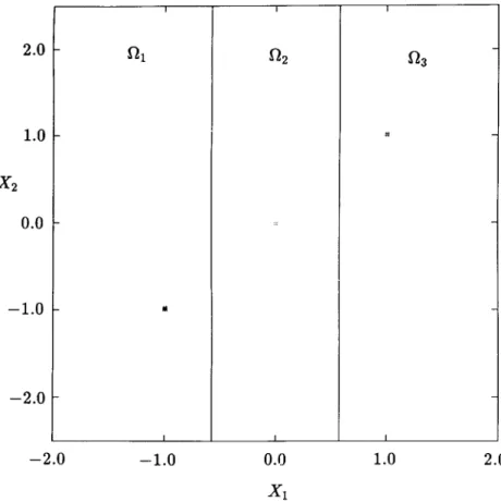
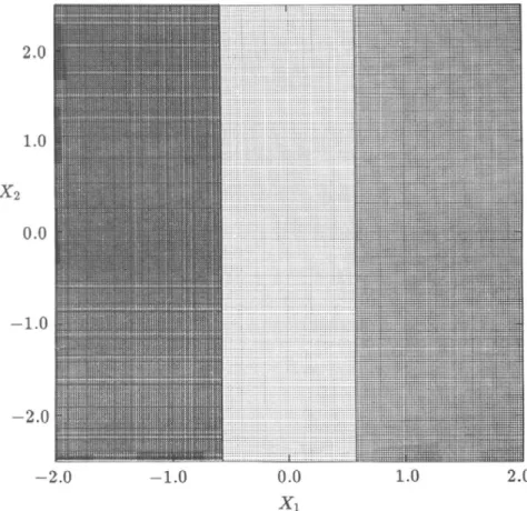
To apply the cell-mapping technique, we cover the phase-plane region - 2 . 0 < X j < 2 . 0 and - 2.5 < x2 < 2.5 with NCi=200 intervals along the
Xj-axis and N = 200 intervals along the x2-axis. This region consists of a total of 40,000 cells with cell sizes ft j — 0.02 and /i2 — 0.025. An associated cell mapping of (2) was computationally obtained by choosing an integration time of T = 0.5 with an integration step size of Ai = T/10. Figure 1 shows the
2.0
1.0
2
0.0
-1.0
- 2 . 0
i
Ox
- *
1
1
n
2i
i
ÍÍ3
»
i
-- 2 . 0 -1.0 0.0 1.0 2.0
FIG. 1. Location of various equilibrium cells for Example 1. Singular manifolds are shown by solid lines.
location of various periodic cells (three different groups each with a core of four equilibrium cells) together with the singular manifolds indicated by solid lines. It is verified that an initial state starting from the center point of an equilibrium cell in each core approaches asymptotically a corresponding equilibrium point of (2). Thus the cell-mapping results lead to the three roots of (26) given by
=C = (0,0), *b* = ( l , l ) , = ( - 1 . - 1 ) . (27)
2.0
1.0
0.0
1 . 0
2 . 0
-i -i -i 1 1 '
- 2 . 0 - 1 . 0 0.0 1.0 2.0
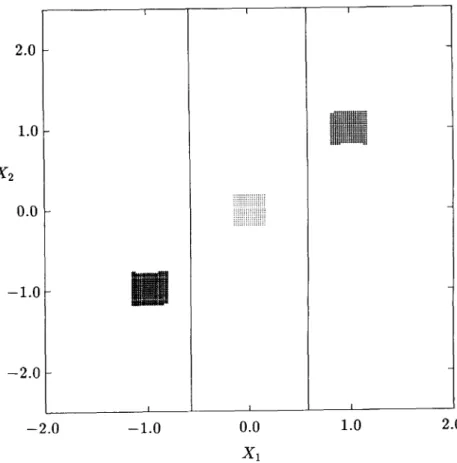
FIG. 2. Four-step domains of attraction of the stable equilibrium points for Example 1.
2.0
1.0
-X,
0.0
- 1 . 0
2.0
-- 2 . 0
1 1 1 1 i
- 1 . 0 0.0
* 1
1.0 2.0
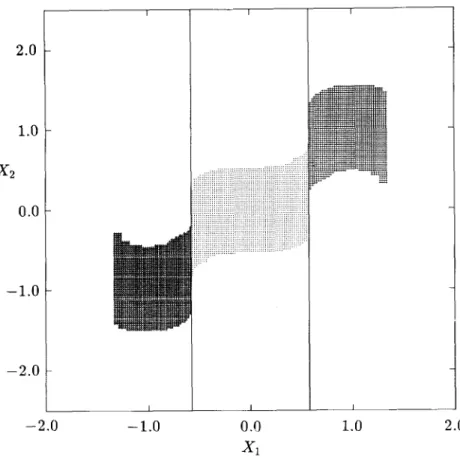
FIG. 3. Six-step domains of attraction of the stable equilibrium points for Example 1.
belong to the domain of attraction of the equilibrium point x*, 11,600 cells to x£, and 14,200 cells to x*. No regular cell is mapped to the sink cell. It should be noted that every domain of attraction of (2) for this problem is included in a different isolated region Í2;., thus confirming analytical results.
EXAMPLE 2. Consider finding the zeros of the vector field / in R2 given by
fi~xi 4x2,
f2 = cosx1-x2.
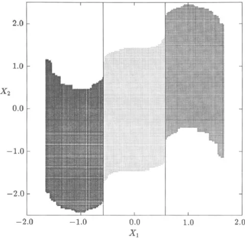
FIG. 4. Eight-step domains of attraction of the stable equilibrium points for Example 1.
We have
F ( x ) = - Xj +4xf +8x2(cosx1 - x2) xl sin xx - 4x1sin xi + c o s xi ~ x2
d e t / ( x )
d e t / ( x ) = - ( l + SxaSinXj).
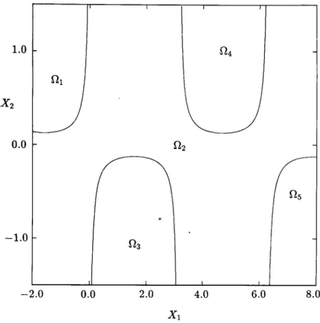
For this example, all the singular manifolds are also barrier manifolds and the isolated regions fl are clearly defined.
FIG. 5. Total domains of attraction of the stable equilibrium points for Example 1.
T = 3 units with integration step size Ai = T/6 is used to generate an associated cell mapping of (2). Three isolated equilibrium cells of the dynami-cal system associated with (2) are obtained. As before, it can be verified that these cells lead to the three roots of / , given by
x* = (3.5021474, -0.9357013),
xb* = (1.0366739,0.5090859),
x* = (2.4764680, - 0.7868399),
(29)
1
-fil 1
-\ -\
ÍÍ3
i
i r
ÍÍ4
l J
ü
2/ ^ 5
1 1
- 2 . 0 0.0 2.0 4.0 6.0 8.0
FIG. 6. Equilibrium cells replacing the stable equilibrium points for Example 2. Singular manifolds are shown by solid lines.
Figure 6, the three asymptotically stable equilibrium points %*, x*, and x* are each replaced by a single equilibrium cell, respectively represented by symbols " •," " X " and " + . " The barrier manifolds are also shown in this figure by the solid lines. It should be noted that the two asymptotically stable equilibrium points x* and x* are included in one isolated region S22, thus supporting the results of Theorem 8.
- 2 . 0 0.0 2.0 4.0 6.0 8.0
Xi
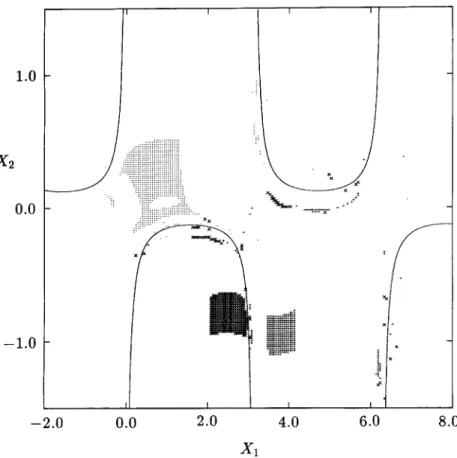
FIG. 7. One-step domains of attraction of the stable equilibrium points for Example 2.
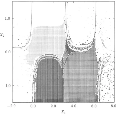
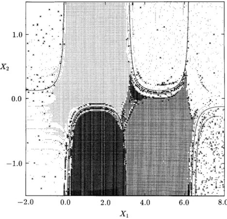
equilibrium cell. Figures 8 and 9 respectively show the two-step and three-step domains of attraction for the stable equihbria. Many cell trajectories, during evolution, may cross the barrier manifolds, as already commented in Section 5. In the evolution of these domains of attraction, notice how more and more of these trajectories are detected. The total domain of attraction is shown in Figure 10, where the largest number of steps required by a cell to get mapped to an equilibrium cell is 12. The domain of attraction of x * contains 13,414 cells, xg has 5347 cells, and x* has 7565 cells, for a total of 26,326. The remaining regular cells, a total of 13,674, map to the sink cell and arc simply indicated by blanks in this figure.
- 1 . 0
0.0 2.0 4.0 6.0
FIG. 8. Two-step domains of attraction of the stable equilibrium points for Example 2. 8.0
manifolds, the cell-mapping results are a very good approximation of the global behavior of the continuous-time dynamical system (2).
EXAMPLE 3. Consider the following algebraic system in R2 taken from Brown [5] and Morgan [24]:
Art X i
/i = ¿ s i n ( * i * 2 ) - ^ - y .
/
2= U
1 \ „ ex2
— \(e*"-e)+ — -2ex1,
air / IT
1.0
X,
0.0
-1.0
- 2 . 0
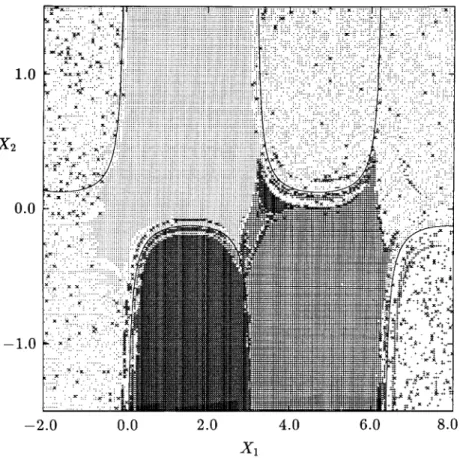
FIG. 9. Three-step domains of attraction of the stable equilibrium points for Example 2.
where e denotes the base of the natural logarithms. For this problem, we have
det J(x) = — [ x a c o s ^ x a ) - l] Á1T
1
2
ll
fi-1
4w \e
1
2x>- - e 2x1 cos(x1x2) I. (31) 77Figure 11 shows the singular manifolds determined by applying the algorithm given in Section 4 to the region - 1.0 < xx < 2.0 and — 20.0 < x2
FIG. 10. Total domains of attraction of the stable equilibrium points for Example 2.
one million cells in the plane) with /ix = 0.003 and h2 = 0.025. The figure
shows the location of cells containing the singular manifolds. The location of the singular manifolds is identical to that obtained in Zufiria and Guttalu [30] by an exhaustive sweeping and iteration in the entire region of interest. The present method cuts down the computational requirements by several orders of magnitude. Also, the method is much simpler to apply and more robust numerically.
We now apply cell mapping to the region — 1.0 < xY < 2.0 and — 20.0 <
x2 < 5.0 by taking Nc = 301 and N = 301 intervals in the region (totaling
90,601 cells) with celí sizes hx = 0.0099667 and h2 = 0.0830564. An
FIG. 11. Singular manifolds and the location of zeros for Example 3. Singular manifolds are shown by solid lines.
(30) discovered by using the location of these cells are given by
x* = (- 0.2605993,0.6225309),
x* = {i,ir),
x* = (1.3374256,
x* = (1.4813196,
x* = (1.5782254,
xfc* = (1.6545827,
-4.1404396),
-8.3836137),
-12.1766999),
-15.8191982),
xg = (0.2994487,2.8369278),
x% = (1.2943605, - 3.1372198),
xf = (1.4339493, - 6.8207653),
x£ = (1.5305053, - 10.2022579),
xf = (1.6045705, - 13.3629027),
FIG. 12. Location of equilibrium cells for Example 3.
FIG. 13. Total domains of attraction of stable equilibrium points for Example 3.
Once again, a fairly clear global picture is provided by the cell-mapping analysis in spite of the uncommon behavior of the dynamical system. The importance of the role played by the barrier manifolds, strongly suggested by theory, is clearly demonstrated in this example. The extent of the domains of attraction is demarcated by the isolated regions in a theoretical sense which is verified numerically by the cefl-mapping method. In addition, it should be noted that parts of some of the barrier manifolds act like an attractor, as seen by the large number of cells which straddle them.
6.2. Application to Finding Fixed Points
EXAMPLE 4. We consider a two-degree-of-freedom nonlinear mechanical system whose response was studied by Hsu [14] and by Hsu and Guttalu [17]. The system consists of two identical rigid bodies free to rotate about a common axis, which are coupled and connected through linear rotational dampers to the stationary support. The two bodies are subjected to simulta-neous periodic impact loads along a fixed direction. The dynamic behavior of this system can be expressed in terms of a point mapping (or discrete dynamical system) defined by x(n + 1) = G(x(n)), where
Gj(x) = xl + Cx(x3 — asin x1 cos x2) ,
G2(x) = x2 + C2(x4 — acos3c1sinx2),
(33) G3(x) = 0^X3 — a s i n x1c o s x2) ,
G4(x) = D2(x4 — acosXjSinXa),
in which
l - e - 2 / n l - e "2" *
C C = D = p'2^ D = P 2^2
2¡X1 2[l2
In (33), xx represents the in-phase mode of oscillations of the system, and x2 the out-of-phase mode of oscillations; x3 and x4 represent their correspond-ing velocities. The dimensionless quantity a is the strength of the impulsive load, and jux and ju2 are the damping coefficients of the in-phase and out-of-phase modes, respectively. It should be noted that the angular dis-placement coordinates x1 and x2 lie in the range — IT < xx < m and — TT < x2 < IT. Since this system is elastically unrestrained, we consider xl mod 2w
and x2mod 2ir.
We present the results for the case a = 5.0, [I1 = 0.1TT, and /¿2 = 0.27r. First, we make use of the compactification function (19) for the angular-velocity components x3 and x4 only. There is no need to compactify the
displacement coordinates xv and x2, because of the periodicity of (33) in
them. By applying the cell-mapping method (taking Nc = 1 1 , Af = 11,
N =31, and NCt = 3l, with T = 0.9 and Ai = T/32) to the compact state
space, we found most of the solutions. The velocity range covered by these solutions provides a good finite estimate of where most of the solutions may be found in the regular state space. The velocity range found was — 1.5w ^ x3 < 1.5w and — 0.5w < x4 < 0.57T. A refined cell mapping was subsequently
applied to this estimated finite velocity range. We now used the state-space region - {IT + h1/2)^x1<{ir+ h1/2), - (77 + h2/2) «S x2 < {IT + h2/2),
— 1.5IT < x3 < 1.577, - 0.5TT < x4 < 0.577, with intervals Nc¡ = 35, N = 35,
2VC3 = 51, JVC4 = 19 (totaling 1,187,025 cells) and cell sizes hx = §v, h2 = ^77,
^3 = ii""' ^4 = w77' an<^ integration parameters T = 1.0, Ai = T/8. Figure 14 shows the location of periodic cells (indicated by the symbol " X " ) deter-mined by this cell-mapping analysis. Center points of periodic cells were used as initial guesses for the Newton-Raphson iterative scheme to numerically
TABLE 1
LOCATION OF P - l SOLUTIONS OF THE MAP G FOR EXAMPLE 4
1( 2( 3( 4( 5( 6( 7( 8( 9( 10( H ( 12( 13( N14( N15( N16( N17( N18( N19( N20( N21( N22( N23( N24( N25( N26( N27( N28( N29( N30( N31( N32( N33( — 77, — TT, — TT, - 0.5T7, - 0.5*7, 0, 0, 0, 0.5w, 0.5T7, w,
" • >
w, -0.577, - 0.5w, 0.5*7, 0.5T7, - 0.5T7, - 0.5*7, 0.5T7, 0.5T7, - 0.710304TT, 0.71030477, - 0.71030417, 0.710304 77, - 0.710304 it,
0.710304 m,
- 0.2896967T, 0.289696 ir, - 0.289696 IT,
0.289696 IT,
- 0.289696TT, 0.289696 77, — IT, 0, 77, - 0.5T7, 0.5TT,
— TT,
0,
TT,
- 0.577,
0.5T7,
— TT,
0,
" • )
- 0.789696 TT,
0.789696 TT, - 0.789696 ir, 0.789696 TT, - 0.210340 TT,
0.210304 TT, - 0.210304 TT,
0.21030477, -TT, — TT, 0,
o,
77, TT, — TT, — TT,o,
0, 77, TT, 0,0 0,0 0,0 0,0; 0,ff 0,0 0,0 0,0 0,0 0,0 0,0 0,0 0,0; -1.4370577,0 -1.4370577,0; 1.4370577,0; 1.4370577,0; 1.4370577,0; 1.4370577,01 -1.4370577,01 -1.4370577,0; -1.4370577,0; 1.43705T7,01 1.4370577,0; -1.4370577,0 -1.4370577,0; 1.4370577,0 -1.4370577,0^ 1.4370577,0; 1.43705 77,0; -1.43705 77, W - 1.4370577,0;TABLE 2
LOCATION OF P-2 SOLUTIONS OF THE MAP G FOR EXAMPLE 4
34( 35( 36( 37( 38( 39( 40( 41( 42( 43( 44( 45( 46( 47( 48( 49( 50( 51( 52( 53( 54( 55( 56( 57( 58( 59( 60( 61(
N 6 2 ( N 6 3 ( N 6 4 ( N 6 5 ( N 6 6 ( N 6 7 ( N 6 8 ( N 6 9 ( N 7 0 ( N 7 1 ( N 7 2 ( N 7 3 ( N 7 4 ( N 7 5 (
0 . 3 3 4 1 9 T 7 ,
- 0 . 3 3 4 1 9 T 7 ,
0, 0,
0.09648 77,
- 0 . 0 9 6 4 8 T T ,
- 0 . 0 9 6 4 8 T T ,
TABLE 2. Continued. N76( N77( N78( N79( N80( N81( N82( N83( N84( N85( N86( N87( N88( N89( N90( N91( N92( N93( N94( N95( N96( N97( N98( N99( N100( N101( N102( N103( N104( N105( N106( N107( N108( N109( N110( N l l l ( N112( N113( N114( N115< N116( N117( 0.21919377, 0.2191937T,
- 0 . 2 4 4 3 7 9 T 7 ,
TABLE 2. Continued. N118( N119( N120( N121( N122( N123( N124( N125( N126( N127( N128( N129( N130( N131( N132( N133( - 0.75562177, - 0.755621W, 0.75562177, 0.75562177, - 0.78080777, - 0.78080777, 0.78080777, 0.78080777, - 0.93388577, 0.93388577, - 0.97277377, - 0.97277377, 0.97277377, 0.97277377, - 0.99207177, 0.99207177, - 0.25554377, 0.25554377, - 0.25554377, 0.25554377, - 0.28662577, 0.28662577, - 0.28662577, 0.28662577, 0, 0, - 0.03941277, 0.03941277, - 0.03941277, 0.03941277, 0, 0, 0.66997677, 0.66997677, - 0.66997677, - 0.66997677, 0.71852577, 0.71852577, - 0.71852577, - 0.71852577, -1.05129177, 1.05129177, - 0.98405377, - 0.98405377, 0.98405377, 0.98405377, 0.92332177, - 0.92332177, 0.18248977) -0.18248977) 0.18248977) - 0.18248977) 0.21334877) -0.21334877) 0.21334877) - 0.21334877) 0) 0) 0.04338977) - 0.04338977) 0.04338977) -0.04338977) 0) 0)
refine the locations of the periodic solutions of the map G. As remarked in Section 5, these periodic cells provided excellent initial estimates for the iterative scheme. The above cell-mapping analysis may be repeated by altering some of the parameters (cell sizes, region of analysis, etc.) until no new solutions are discovered. P-1 solutions thus obtained are listed in Table 1, and P-2 solutions in Table 2. The symbol " N " in these tables indicates a new solution found by the present method. Figure 15 shows the location of these solutions in the xrx2 plane. P-1 solutions are represented by the symbol
" X ," and P-2 solutions by " O . "
In all, there are 133 periodic points in Tables 1 and 2; 33 of them are P-1 points and 100 are P-2 points; that is, there are 50 P-2 solutions. In Hsu and Guttalu [17], a method based on simplicial mapping and cell functions was employed to determine P-1 and P-2 solutions of the map G. In comparison with their solutions, we have discovered 20 new P-1 points and 72 new P-2 points. Altogether, by using the method developed in this paper, 92 new roots of the vector function /( 2 ) have been discovered.
Next, we carried out a study to check whether solutions other than those listed in Tables 1 and 2 may be found by other numerical procedures. One such procedure is a heuristic search in the state space. Of course, this search may not give all the roots. However, if a random search does not provide a new root, then the results obtained by the present method are strengthened. We applied Newton's iterative method to find the roots of the function f<2)
7T 0.57T 2 0.0 0.57T — •K i 0 l -0 Y 0 0 - Y-0 i 1 «—e 0 0 0 0 0 X 0 0 o 0 0
1 a. -e
— r - e * - ,
X 0 0 o 0 X X 0
0 O X )
0 X X 0 0 0 0 X
l o » 1 . e—^B—e 0 0 0 0 0 X 0 0 0 V e—SB—e
p-x e-| o * > |
0 X 0 0 0 X 0 o 0 0 X 0
CX 0 0 X
0 X 0 0 o 0 X 0 <9 0 o X 0
1—* p i 0 IP 1
0 -0 0 •< 0 -0
— 7T - 0 . 5 7 T 0.0 0.57T 7T
X,
FIG. 15. Location of P-l and P-2 solutions in the x¡-x2 plane for Example 4.
Separate trials were made for three different regions covering the velocity ranges (a) - 5 < x3 < 5, - 5 < x4 < 5, (b) - 50 < x3 < 50, - 50 < x4 < 50,
and (c) - 500 < x3 < 500, - 500 < x4 < 500. In each case, a total of one
million initial guesses were used. With these trials we found no new root of the function /<2).
7. CONCLUDING REMARKS
guesses which may prove useful for iterative and homotopic techniques when they are employed for the purpose of refining the location of the roots.
The singular manifolds of the dynamical system, as explained in Zufiria and Guttalu [30], play a definitive role in characterizing its global behavior. Theoretical results are presented in this paper utilizing a discrete state space to support a numerical algorithm for locating the singular manifolds. The algorithm has been implemented and is found to be simple, robust, and computationally very efficient. In general, this algorithm can be used to find zeros of a scalar function of many variables.
The capability of the methods presented in this paper is illustrated by examples provided in Section 6. It appears that, as long as the cell sizes are made small enough to contain only one root in a cell, all the roots are recovered. Application of the method to a mechanical system provided many more solutions than those previously discovered, thus demonstrating the utility of the computational scheme outhned here. This approach presented in this paper for determining the singular manifolds was successfully tested in Example 3.
The computational robustness of the cell-mapping method in dealing with uncommon dynamical systems has been demonstrated in this paper. Both the cell-mapping method and the algorithm for locating the singular manifolds have enabled us to validate the results given by Zufiria and Guttalu [30]. Especially, the importance of the singular manifolds in delineating the domains of attraction has been highlighted.
The computational methods developed in this paper can be applied in the same spirit to any other dynamical system which can be formulated for the purpose of finding the zeros of vector functions. In the same way, the method is applicable to any dynamical system developed for solving global optimiza-tion problems.
The work reported here is partially supported by a grant from the National Science Foundation Grant under EET-8709267. P. J. Zufiria wants also to acknowledge the support of a Formación de Post grado fellowship of the Programa Nacional de F.P.I, provided by the D.G.I.C.T. of the Ministerio de Educación y Ciencia of Spain.
REFERENCES
1 O. Axelsson, On global convergence of iterative methods, in Iterative Solutions of Nonlinear Systems of Equations (R. Ansorge, Th. Meis, and Tornig, Eds.), Springer-Verlag, New York, 1982.