Explaining heavy vehicle demand evolution in toll roads:
A dynamic panel data approach in Spain
Juan Gómez
PhD. Candidate, Centro de Investigación del Transporte (TRANSyT-UPM)
José Manuel Vassallo
Associate Professor, Centro de Investigación del Transporte (TRANSyT-UPM)
ABSTRACT
Improving the knowledge of demand evolution over time is a key aspect in the evaluation of transport policies and in forecasting future investment needs, specially critical for the case of toll roads. However, literature regarding demand elasticity estimates in toll roads is sparse and leaves some important aspects to be analyzed in greater detail. In particular, previous research does not focus on heavy vehicle demand, so that the specific behavioral patterns of this traffic segment are not taken into account. Furthermore, GDP is the main socioeconomic variable most commonly chosen to explain road freight traffic growth over time. This paper seeks to determine the variables that better explain the evolution of heavy vehicle demand in toll roads over time. To that end, we present a dynamic panel data methodology aimed at identifying the key socioeconomic variables that explain the behavior of road freight traffic throughout the years. The results show that, despite the usual practice, GDP may not constitute a suitable explanatory variable for heavy vehicle demand. Rather, considering only the GDP of those sectors with a high impact on transport demand, such as construction or industry, leads to more consistent results. The methodology is applied to Spanish toll roads for the 1990-2011 period. This is an interesting case in the international context, as road freight demand has experienced an even greater reduction in Spain than elsewhere, since the beginning of the economic crisis.
1. INTRODUCTION
socioeconomic explanatory variable in the analysis.
The aim of this paper is to contribute to a better knowledge of heavy vehicle demand on interurban toll roads by identifying some of the key socioeconomic variables influencing traffic evolution. Through an original methodology, we discuss the suitability of GDP as a socioeconomic explanatory variable of road freight traffic on toll roads, and propose alternative variables that better explains the evolution of road freight demand over time. Additionally, this paper analyzes the effects of the economic crisis on heavy vehicle demand for toll roads, and tests the suitability of the explanatory variables chosen.
The methodology is applied to the Spanish toll road network, which represents a very interesting case in the international context. The deterioration of the economic environment in Spain since 2008 has had a great impact on the level of traffic in the tolled network, particularly as regards heavy vehicle demand. According to data from the Spanish Ministry of Transportation (Ministerio de Fomento, 2013), heavy vehicle demand in toll roads has fallen, since the beginning of the crisis, by a full 40%. As a result, road freight demand has returned to levels of 1994, when the tolled network was 46% smaller.
This paper is organized as follows. After the introduction in Section 1, Section 2 summarizes the state of knowledge regarding heavy vehicle demand on interurban roads. Section 3 establishes the methodology of this research, by describing both data series and the panel data models used to estimate demand elasticities. Section 4 presents and discusses the results. Finally, Section 5 sets out the main conclusions and suggests avenues of further research.
2. STATE OF KNOWLEDGE
Existing research on the evolution of traffic has focused on light vehicle demand, while road freight traffic has received little attention. Basically, the responsiveness of road demand with respect to different factors is measured through the concept of elasticity, by definition the relative change in travel demand induced by a relative change in a certain explanatory variable.
2.1Previous research for free roads
with facility location and urban form (Allen et al., 2012) and estimates of external costs for intercity freight trucking (Forkenbrock, 1999). Finally, few studies have analyzed, through a macro approach, the relationship between heavy goods vehicle demand and certain explanatory variables in countries such as the US (Gately, 1990), Australia (Li et al., 2009) or Portugal (Matos et al., 2011). Furthermore, recent experiences (Kveiborg et al., 2007) have suggested that the relationship between GDP and heavy goods vehicle demand may not be as enduring as often supposed (McKinnon, 2007).
2.2Previous research for toll roads
As mentioned before, literature regarding road freight demand for toll roads is still limited and focuses mainly on urban and metropolitan areas (Arentze et al., 2012). However, only a very few papers can be found regarding heavy vehicle demand in interurban toll roads, and they are focused on experiences in just a few nations. In the case of the United States, the most consistent research was conducted by Burris et al. (2011), who analyzed a sample of 12 interurban and metropolitan toll roads throughout the nation during an 11-year period (2000-2010). They found statistically significant results for heavy vehicle demand elasticities with respect to tolls (-0.35), with fuel price elasticities ranging from -0.22 to +0.14. Taft (2004) estimated a toll elasticity of -0.59 for truck volume on the Ohio Turnpike, while Holguín-Veras (2003) analyzed toll lanes for exclusive use by heavy trucks on Southern California.
Regarding Norway, Odeck et al. (2008) calculated the elasticity of travel demand in 19 Norwegian toll road projects, and calculated an average toll elasticity of -0.51 for heavy goods vehicles. Hensher et al. (2013) investigated the response of road freight operators in Australia to price signals under different charging schemes, defined by combinations of distance, mass and location. For the case of Spain, Álvarez et al. (2007) estimated the value of time and travel elasticities for both a Spanish toll motorway and its free parallel road, finding statistically significant elasticities for tolls (-0.39) and fuel prices (-0.09).
The existing literature on interurban toll roads leaves some important aspects to be investigated. First, previous studies have paid little attention to road freight traffic in tolled infrastructure. Furthermore, statistic models developed hardly establish a macro approach to quantify the relationship between road freight demand evolution and economic growth over time, as well as to identify the key explanatory variables of heavy vehicle traffic. In this respect, it is necessary to assess to what extent GDP constitutes a suitable explanatory variable for heavy goods vehicle demand in toll roads, and to explore possible alternatives. For the case of Spain, no previous studies have been undertaken specifically to investigate heavy vehicle traffic evolution.
This section presents the data collected for the analysis of heavy vehicle demand on Spanish toll roads, as well as the methodology we followed to develop the dynamic panel data approach.
3.1Previous data analysis
In order to estimate the demand equation for heavy vehicle traffic, we establish a dynamic panel data corresponding to 14 Spanish toll roads observed between 1990 and 2011. The sample includes those toll highways whose traffic data series are long enough for the statistical approach adopted in this paper, which is described below. Every toll highway included in the sample has a free parallel conventional road competing with it. The analysis thus focuses on toll roads with a free alternative of lower quality.
The dependent variable of the demand equation is the annual average daily traffic volume (AADT) for heavy vehicles in each toll road. These data have been collected from the statistics of the Spanish Ministry of Transportation (Ministerio de Fomento, 2012). Although traffic data from shorter tolled sections were available, we have only considered average data for entire toll roads in order to avoid spatial correlation problems in the models.
Dependent variable
Explanatory variables
Previous demand
Socioeconomic Generalized cost
Toll Fuel
AADT
(Heavy Vehicles) AADT (-1)
• GDP (provincial)
Toll prices (heavy vehicles)
Fuel cost (€/km): Diesel prices & Efficiency • GDP (national)
• Construction & Industry GDP (prov.) • Construction & Industry GDP (national) • Industry GDP (prov.)
• Industry GDP (national)
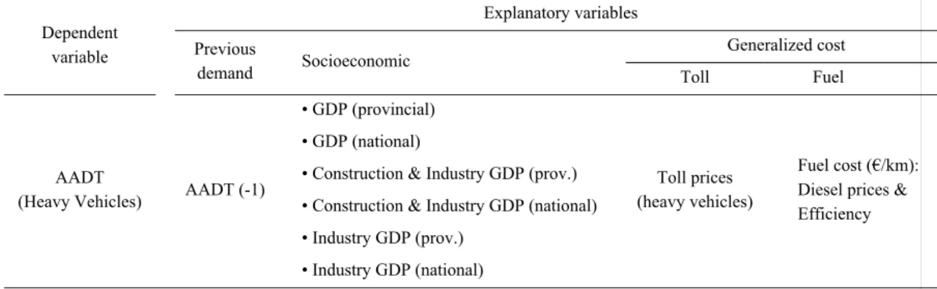
Table 1 – Explanatory variables included in the analysis
Three kinds of explanatory variables have been included in the demand equation (see Table 1): demand volume of previous years, socioeconomic variables, and generalized cost parameters. The demand variable (AADT(-1)) consists of a lag of the traffic volume, a term
needed due to the dynamic nature of the panel. Within socioeconomic variables, we have considered several alternatives. Firstly, we take GDP since it is the most common socioeconomic variable used to explain road freight traffic growth. Secondly, we consider combined GDPs only of transport-intensive activities, particularly Construction and Industry (GDPC+I). This variable exclude those sectors with little or no impact on road
demand, such as financial services, public administration, education, etc. Finally, GDP of the industrial sector alone (GDPInd) is included, as greater influence on toll road traffic can
commodities, with lower toll elasticities according to EPA (2011). By contrast, construction activities in Spain are mainly of an intra-regional nature (Vassallo et al., 2013), so that a smaller impact on toll road traffic can be expected. Data have been collected from the Spanish National Statistics Institute (INE). Other socioeconomic variables, such as population or size of the vehicle fleet, have been discarded, as weaker relations with traffic have been observed for these, especially after the beginning of the economic crisis of 2008.
As mentioned before, three kind of explanatory variables are included in the demand equation: previous demand, socioeconomic and generalized cost variables. Specifically, the equation incorporates a lag of the traffic volume (AADT(-1)), a Socioeconomic variable and
two Generalized cost parameters (Toll and Fuel), what results in a total of 4 categories:
AADT = f (AADT(‐1), Socioeconom., Toll, Fuel) (1)
According to Table 1, we consider several alternatives within these four categories, particularly in the socioeconomic one. This methodology then allows us to calibrate several models just by taking one variable from each of the groups of the demand equation. This variability improves the analytical capability of the methodology applied. Further details of the demand equation and the methodology are provided in Section 3.2.
Regarding socioeconomic variables, two levels of data have been considered in the analysis: provincial level and national level. With the aim of better measuring the influence of local socioeconomic characteristics on heavy vehicle demand, data have been collected at the provincial level. In this respect, each toll road is assigned the socioeconomic data from the provinces it crosses. Furthermore, data at the national level have also been tested since the panel analysis is applied to different toll roads spread throughout the country. Monetary socioeconomic variables (total GDP and combined GDPs of certain sectors) have been deflated by the Consumer Price Index (CPI) to reflect their real value over time.
With regard to Generalized cost variables, historical toll rates –expressed in euro/km– were collected from the statistics of the Spanish Ministry of Transportation (Ministerio de Fomento, 2012). A Fuel cost variable is established by taking into account not only diesel prices –expressed in euro/liter– but also fuel consumption (liter/km) for heavy vehicles. It allows us to reflect real fuel costs when driving (euro/km) and include the rebound effect due to the progression in fuel efficiency experienced by trucks over time. Both toll rates and fuel costs have been adjusted to inflation by using the CPI.
heavy vehicle demand.
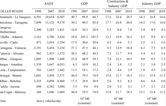
Table 2 provides an overview of the evolution of some of the provincial socioeconomic variables for all the toll roads selected before and after the economic recession. The figures show the long and strong economic growth experienced in Spain during the 1990-2007 cycle, when national GDP increased by 78.0%. For the provinces crossed by the toll roads selected, the data shows average growth rates of 76.5% for total GDP, 54.7% for GDPC+I,
and 34.6% for GDPInd. This period of prosperity has been followed by a significant
deterioration since 2008. National GDP fell by 7.4% between 2007 and 2011. Provincial socioeconomic data also shows significant average reductions from 2007 to 2010 for total GDP (-5.2%) as well as for GDPC+I (-16.0%) and GDPInd (-15.2%).
AADT GDP Construction &
Industry GDP Industry GDP
TOLLED ROADS 1990 2007 2010 1990 2007 2010 1990 2007 2010 1990 2007 2010
Montmeló - La Jonquera 4,591 10,654 8,207 49.7 89.9 84.7 17.6 24.4 20.5 14.3 16.8 14.6
Barcelona - Tarragona 7,099 13,125 9,179 50.3 90.5 85.4 17.7 24.8 20.8 14.5 17.0 14.8
Zaragoza -
Mediterráneo 2,300 2,287 1,421 16.8 30.3 28.9 5.2 8.4 7.0 3.9 4.9 4.5
Villalba - Adanero 2,161 4,786 3,434 54.8 105.2 101.5 12.3 19.9 16.2 8.5 9.9 8.1
Sevilla - Cádiz 471 2,016 1,354 17.5 30.6 28.6 4.2 6.6 5.1 2.5 3.1 2.6
Tarragona - Valencia 2,191 5,454 3,234 27.1 47.5 44.1 8.3 12.9 10.4 6.3 7.5 6.5
Valencia - Alicante 982 2,433 1,372 26.5 48.2 44.2 7.3 11.7 9.4 5.4 6.3 5.4
Bilbao - Zaragoza 1,002 1,890 1,448 23.4 40.9 39.3 7.4 12.3 10.5 6.0 8.3 7.3
Burgos - Armiñón 1,339 5,647 4,033 6.3 10.9 10.2 2.4 3.8 3.2 2.1 3.0 2.5
León - Campomanes 703 1,655 1,442 11.5 18.1 17.2 2.8 4.6 3.9 1.8 4.5 2.0
Montgat - Mataró 1,601 3,438 2,571 44.4 79.5 74.9 15.8 21.7 18.3 13.1 15.4 13.3
Bilbao - Behobia 2,235 4,894 4,460 17.5 29.8 28.9 5.6 9.2 8.2 4.6 6.4 6.0
Tudela - irurzun 698 4,382 3,694 5.5 9.6 9.6 2.0 3.2 3.1 1.7 2.3 2.2
San Cugat - Manresa 366 1,696 1,069 44.4 79.5 74.9 15.8 21.7 18.3 13.1 15.4 13.3
Units heavy vehicles/day 10
3 M€
(constant)
103 M€
(constant)
103 M€
(constant)
Table 2 – Average heavy vehicle demand for Spanish tolled motorways considered and provincial socioeconomic data (1990-2010)
Heavy vehicle demand has experienced trends similar to those of socioeconomic variables. Road freight traffic rose on average by 188.1% over the period 1990-2007, in line with the economic growth in the country. Trends have changed since the beginning of the crisis, and demand levels in 2010 were 27.7% lower than the peak reached in 2007. These sharp variations observed in the tolled network during the last 20 years make Spain an interesting case to be analyzed as well as useful in testing the robustness of the models.
3.2Dynamic panel data methodology specification
heavy vehicle demand in toll roads. It allows us to estimate demand elasticities with respect to explanatory variables included in Table 1. All variables are expressed in logarithms. The form proposed for the estimation models is:
,
With provincial socioeconomic data: t = 1990, …, 2010; i = 1, …, 14
With national socioeconomic data: t = 1990, …, 2011; i = 1, …, 14
(2)
Given the dynamic nature of the analysis, the equation includes a lag of the demand variable (AADTt-1). Fuel denotes fuel costs assumed by trucks in euro/km. Tollit denotes
toll rate (euro/km) applied in road i for year t. Finally, Socioecit denotes different
socioeconomic data (total GDP, GDPC+I and GDPInd) assigned to road i, either at the
provincial or national level. Regarding the rest of the parameters, βk is the short-run
elasticity of road demand with respect to explanatory variable k; λ measures possible autocorrelation in traffic data series; ηi denotes unobserved individual effects, that is,
constant and specific factors for each tolled road, not accounted for by any of the other variables in the models; finally, εit is the residual or idiosyncratic error.
Regarding initial conditions, we assume (Blundell et al., 1998) that ηi and εit are
independently distributed across i and have the familiar error components in which:
E(ηi) = 0, E(εit) = 0, E(ηi εit) = 0 for i = 1,…,N and t = 2,…,T.
E(εit εis) = 0 for i = 1,…,N and t ≠ s.
(3)
As pointed out by Graham et al. (2009), the main issue to be addressed in the context of dynamic panel estimation is correlation between the lagged dependent term (AADTi,t-1)
and the unobserved cross-section individual effects (ηi). This fact greatly limits estimators
to be applied. The Ordinary Least Squares (OLS) estimator for λ is then inconsistent (Bond, 2002) and biased upwards (Blundell et al., 2000). The Within Groups (WG) estimator clears this source of inconsistency by transforming the equation to eliminate ηi,
but gives an estimate of λ that is biased downwards, especially in short panels (Bond, 2002). Therefore, a consistent estimate of λ can be expected to lie between the OLS and WG estimates (Arellano et al., 1991). However, better estimates can be calculated with a Generalized Method of Moments (GMM) approach, specifically through the proposed difference GMM estimator (GMM-DIFF), which includes an instrumental variables (IV) approach (Arellano et al., 1991).
The GMM-DIFF estimator assumes that values of the dependent variable lagged two periods or more (AADTi,t-s, for s ≥ 2) are valid instruments for the lagged dependent
variable in the differenced equation, Δ(AADTi,t). That is, assuming a set of instrumental
variables which are correlated with Δ(AADTi,t-1) but orthogonal to the differenced
problems that can arise when too many instruments are considered (Roodman, 2009), we have opted for using only the first lag available in each time period. Furthermore, according to Judson et al. (1999), limiting the number of instruments does not materially reduce the performance of this technique. The GMM-DIFF approach generates consistent and efficient estimates of the parameters (Rey et al., 2011), among other attractive properties noted in the literature (Graham et al., 2009), but the instrumental variables estimator performs poorly as the value of λ increases towards unity, particularly at values above 0.8 (Blundell et al., 1998).
To overcome the weak instrument problem for persistent series, Arellano et al. (1995) and Blundell et al. (1998) suggested a system GMM estimator (GMM-SYS). It establishes a system of equations in both first differences and levels, where the instruments used in the levels equations are lagged first differences of the series. The GMM-SYS approach can reduce the finite sample bias of results, improves the precision and constitutes a more efficient estimator (Arellano et al. 1995). However, despite being smaller, the finite sample bias of the GMM-SYS estimator is generally upwards, in the direction of OLS levels (Blundell et al., 1998). Finally, it must be noted that the most suitable technique in each case can change depending on the size of the panel (Judson et al., 1999).
The most widely used tests to check the validity of hypotheses assumed in GMM estimators are the m1 and m2 tests, as well as the Sargan test (González et al., 2012). The m1 and m2 tests, proposed by Arellano et al. (1991), detect first and second-order serial correlation problems in Δεit, respectively. Both tests are generally used to check that no
serial correlation is observed in the estimated residuals εit. Additionally, the Sargan test
checks the validity of the instruments used in the model. Asymptotically distributed as a chi-square under the null of instrument validity, it detects possible correlation between the instruments and differenced residuals Δεit. However, as noted by Böckerman et al. (2009), the Sargan test can have extremely low power when using too many instruments in the GMM model, so we have adopted the alternative procedure proposed by Roodman (2009) of using only the first lag for instrument in the demand equation.
4. MODELLING RESULTS AND DISCUSSION
4.1General aspects
This paper develops an original approach to identify the key socioeconomic explanatory variables influencing road freight traffic. This research is based on estimates of demand elasticities with different panel data models including some new aspects in our analysis:
the period of analysis is extended. Then, those variables with significant variations in their demand elasticities over time cannot be considered as suitable to explain the evolution of road demand.
• As mentioned above, the methodology includes a great variety of explanatory variables with regard to socioeconomic data, period of time considered, size of the sample, etc. This variety enables a direct and deeper comparison of available alternatives, and makes it easier to identify which variables explain road demand evolution in a better way.
• Very little research on toll road demand has included the period of economic crisis in the analysis. Studying such an interesting case as the Spanish tolled network, allows us to test the robustness of the results when the economic outlook changes dramatically.
The great diversity of models presented in the methodology does not make it possible to show the results for each and every one of the alternatives available. In this paper, we focus on the behavior of some variables, especially socioeconomic ones due to their great explanatory potential for road demand. Furthermore, different figures summarize the evolution of demand elasticities as described above, in order to make the analysis more appealing and easier to grasp. The following subsection presents and discusses the most interesting results from all the models considered in the analysis.
4.2Analysis of explanatory variables influencing heavy vehicle demand
This subsection summarizes the estimates of heavy vehicle demand elasticities by using the panel data methods described before (OLS, WG and GMM), when taking into account all the variables considered according to Table 1. Results are sorted by socioeconomic variables (total GDP; Construction & Industry GDP, GDP C+I; and Industry GDP, GDPInd), as they may be the key explanatory variables of demand evolution.
Table 3 includes detailed results for a certain demand model applied to e.g. the 1990-2007 period when considering provincial GDP, toll rates and fuel cost (€/km) as explanatory variables for heavy vehicle traffic. According to Arellano et al. (1991), the λ estimates for OLS-pool (0.985) and WG (0.203) are biased upwards and downwards, respectively. Regarding the GMM-DIFF estimator, the elasticity result (0.379) comfortably falls between that of OLS and WG, and is significantly different from zero. However, the λ
estimate for the GMM-SYS estimator (0.975) is very close to that from the OLS-pool, which suggests some kind of bias in the results. This has been a circumstance frequently met with in conducting the analysis, so in the end we have chosen the GMM-DIFF approach for the analysis.
OLS - pool WG fixed effects GMM - DIFF GMM - SYS Estimate p-value Estimate p-value Estimate p-value Estimate p-value AADT (-1) 0,985 0,0000 0,203 0,0000 0,379 0,0007 0,975 0,0000 GDP (prov.) -0,007 0,3970 2,000 0,0000 0,925 0,0000 0,001 0,9459 Fuel cost 0,169 0,3758 -0,102 0,0061 -0,431 0,0013 -0,052 0,5286 Toll -0,025 0,0062 -0,220 0,0000 -0,334 0,0044 -0,049 0,2042
R2 0,9856 0,3848
m1 - test -1,556 0,0498 -1,822 0,0341
m2 - test -0,010 0,4956 -1,576 0,0574
Sargan test 14,0 0,5255 14,0 0,9990
Table 3 – Estimation of travel demand elasticities for the 1990-2007 period, through different panel data estimators
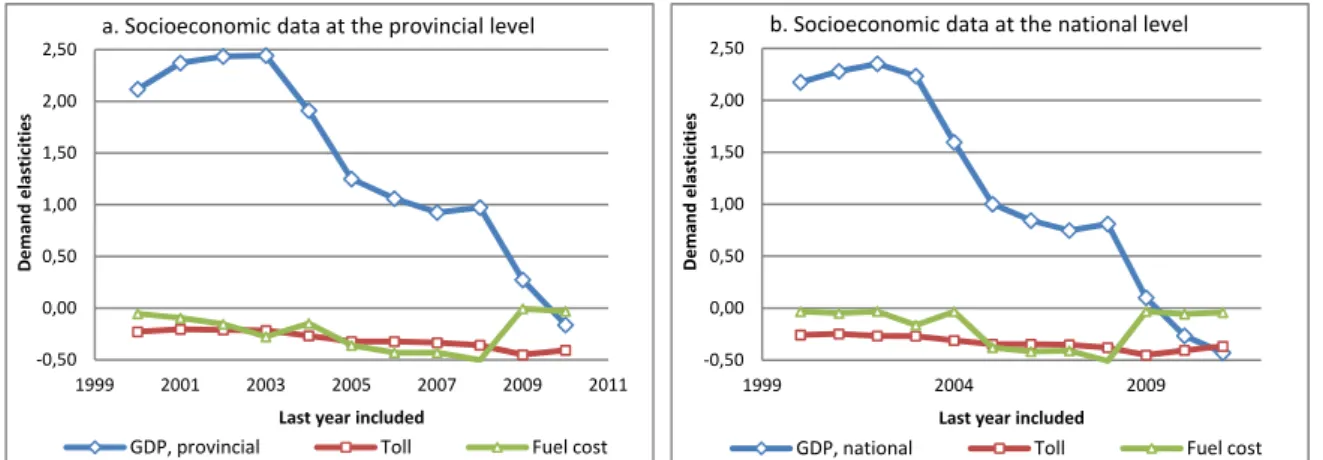
Previous studies often conclude their research at this point. We now introduce some variability by calibrating new models with time periods progressively extended over time. An illustrative example can be seen in Figure 1. It shows elasticity results from models including toll rates, fuel cost and total GDP either at a provincial level (subfigure 1.a) or at a national level (subfigure 1.b) as explanatory variables. Furthermore, each subfigure reveals how demand elasticities vary when the time period considered changes over time. The y-axis measures demand elasticities. The x-axis indicates the last year considered in the time period, taking 1990 as the starting point, so it allows for the analysis of the evolution of travel elasticities when an additional year is included in the model. Therefore, subfigures show how elasticities change when the time period gradually varies from 1990-2000 to 1990-2010. It can be easily seen that results shown in Table 3 are displayed in subfigure 1.a (provincial data) in the right-hand side, specifically for x=2007. As can be noted, all the elasticities have the expected sign: negative for both Toll and Fuel costs and positive for GDP, except in the period since 2010. We want to draw the attention to the great analytical capability of Figure 1. As can be seen, it enables quick and simultaneous comparisons of results for 23 different models (11 and 12 models for provincial and national socioeconomic data, respectively), which makes it easier both to observe trends and to identify key explanatory variables.
Fig. 1 – Demand elasticities when considering provincial GDP (left) and national GDP (right) as the socioeconomic variable in the model
‐0,50 0,00 0,50 1,00 1,50 2,00 2,50
1999 2001 2003 2005 2007 2009 2011
Demand el asti ci ti es
Last year included
a. Socioeconomic data at the provincial level
GDP, provincial Toll Fuel cost
‐0,50 0,00 0,50 1,00 1,50 2,00 2,50
1999 2004 2009
Demand el asti ci ti es
Last year included
b. Socioeconomic data at the national level
In Figure 1 we observe that results are very similar when considering socioeconomic data either at the provincial or at the national level. Secondly, if we observe the evolution of demand elasticities with respect to GDP, different periods are identified:
• Until 2003, demand elasticity moves around 2.0-2.5, which is above the usual values found in the literature. We should note that these results correspond to the peak in the economic growth experienced by Spain during the 1990s and early 2000s.
• Next, GDP elasticities significantly decrease when including the 2004-2009 period. Results range from 0.81 to 1.24, which is in line with previous studies for road freight traffic (Matos et al., 2011; Gately, 1990). The decline observed makes clear that, once a certain level of economic development is reached, further growth causes smaller increases in road traffic. Additionally, some kind of decoupling effect may appear as a result of the use of larger vehicles, increasing average loads, etc. (Kveiborg, 2007), as well as declining share of transport-intensive activities in GDP.
• Finally, GDP elasticities fall sharply after the beginning of the economic crisis, with values near zero or even negative. These inconsistent results seem to show that the models are not able to provide a satisfactory explanation for the road freight traffic reduction in Spain, when total GDP is the socioeconomic variable chosen.
Figure 1 shows that demand elasticity with respect to total GDP experiences great variability over time. As pointed out by Matas et al. (2012), it is often unrealistic to assume a constant elasticity for certain explanatory variables. However, the huge variability of results for total GDP greatly weakens its capability to explain heavy vehicle demand, as both variables show no stability over time. GDP elasticities move from -0.16 to 2.44 when considering provincial data, and range from -0.43 to 2.35 when choosing GDP data at the national level. This makes clear that total GDP does not represent a suitable explanatory variable to be considered as useful in predicting road freight traffic evolution in toll roads. Results for toll and fuel elasticities are not commented here, since including total GDP as an explanatory variable in the models does not lead to good estimates. Nevertheless, detailed results for toll and fuel elasticities are commented upon below, when we present more consistent models.
Figure 2 includes estimates when considering Construction & Industry GDP (GDPC+I),
either at the provincial (subfigure 2.a) or the national level (subfigure 2.b), for the socioeconomic variable in the model. Unlike total GDP, results for GDPC+I show great
stability when gradually varying the time period. Demand elasticities move between 0.74 and 1.32 with provincial data, and range from 0.53 to 0.79 when taking national data.
demonstrates that GDPC+I is a more suitable explanatory variable. It contrasts with the
results shown for GDP elasticities, with greater variability over time. Some reasons for this can be set. While total GDP consists of the aggregation of different heterogeneous sectors of the economy, GDPC+I could be a better proxy for road freight mobility. It only refers to
transport-intensive sectors (Construction and Industry) and excludes those activities with little effect on road demand: public administration, financial services, etc.
Fig. 2 – Demand elasticities when considering provincial Construction & Industry GDP (left) and national Construction & Industry GDP (right) as the socioeconomic variable in the model
Figure 2 also demonstrates that changes in heavy vehicle demand trends on Spanish toll roads during the economic crisis cannot be considered an anomalous fact, despite sharp reductions suffered since 2007. GDPC+I elasticities in recent years move in the usual range
of values of previous years and, therefore, nothing can be concluded in this respect. It makes clear that, if proper explanatory variables are chosen, elasticity estimates show a fairly continuous trend despite dramatic changes in the economic outlook. Furthermore, we want to point out that subfigures 2.a and 2.b present quite similar results. We could initially expect better performance for provincial data, as they have a stronger relationship with local, specific factors for each road. Nevertheless, GDPC+I data at the national level have
also been shown to be a good proxy for the whole tolled network. This good performance of national GDPC+I as an explanatory variable for road freight transport can be attributed to
the high proportion of long trips in the tolled high capacity network in Spain, as goods – mainly industrial commodities– need to be transported from the industrialized regions near the coast and distributed throughout the inner part of the peninsula.
Next, results concerning demand elasticities with respect to toll rates and fuel costs are set out. Toll elasticities show a quite stable trend, with values moving from -0.25 to -0.45 and a mean of -0.32, which is consistent with previous research (Burris et al., 2011; Álvarez et al., 2007). This behavior is likely caused by the fact that real toll rates in the sample remain quite stable, as toll rates in Spain are usually adjusted through inflation. It is also noted that toll elasticities increased slightly over time, especially since the beginning of the economic crisis. Regarding fuel elasticities, greater variations are observed. Estimates move from
-‐0,50 0,00 0,50 1,00 1,50 2,00 2,50
1999 2001 2003 2005 2007 2009 2011
Demand el asti ci ti es
Last year included
a.Socioeconomic data at the provincial level
GDP C+I, prov Toll Fuel cost
‐0,50 0,00 0,50 1,00 1,50 2,00 2,50
1999 2004 2009
Demand el asti ci ti es
Last year included
b. Socioeconomic data at the national level
0.05 to -0.56, averaging -0.24. A wide variety of results are also observed in the literature, as fuel elasticity estimates range from -0.41 (Gately, 1990) to values near zero (Álvarez et al., 2007) or even positive (Burris et al., 2011). Our values are in line with previous results, as they usually fall between the highest and lowest estimates found in the literature review. Although the relative position of toll and fuel curves can change over time, both elasticities show values of the same order of magnitude. Nevertheless, it seems that user´s perception toward tolls is slightly higher than that of fuel costs.
Figure 3 includes elasticity results when Industry GDP (GDPInd) is the socioeconomic
variable in the model. It constitutes the most solid alternative, as all demand elasticities – socioeconomic, tolls and fuel costs– present very constant results. GDPInd turns out to be a
very stable explanatory variable. Elasticities run from 0.91 to 1.20 with provincial data, and from 0.55 to 0.90 with national data. Despite some volatility experienced for particular years, the behavior of GDPInd can be considered highly satisfactory.
Fig. 3 – Demand elasticities when considering provincial Industry GDP (left) and national Industry GDP (right) as the socioeconomic variable in the model
Elasticities with respect to toll rates and fuel costs also show significant stability. Trends for toll elasticities are very constant and values move around -0.25, while those for fuel elasticities are generally lower and lie between 0.0 and -0.24. These results reinforce the notion that the perception of tolls by users is slightly higher than that of fuel costs.
4.3Analysis of explanatory variables influencing heavy vehicle demand
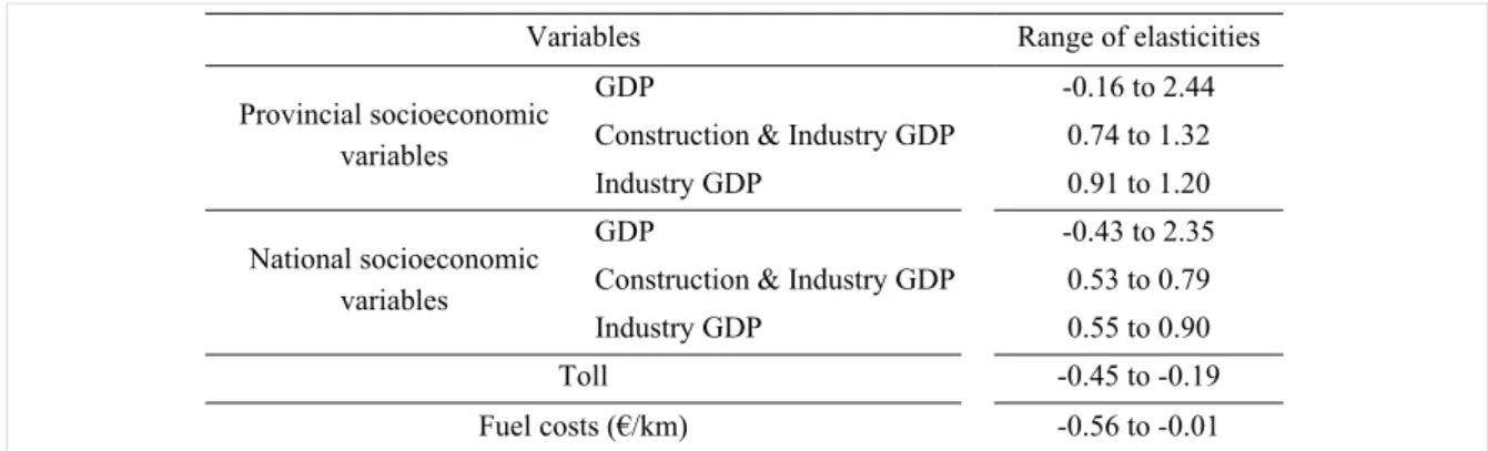
Finally, Table 4 summarizes the main elasticity estimates calculated through this panel data approach. As the analysis over time has evidenced, a range of figures seems a more complete and fairer way to present results for demand elasticities, rather than the traditional approach of simply showing a single value for each variable. It gives essential information for traffic forecasts, since it can be generally assumed that the shorter the range of elasticities, the greater its usefulness as an explanatory variable.
‐0,50 0,00 0,50 1,00 1,50 2,00 2,50
1999 2001 2003 2005 2007 2009 2011
Demand
el
asti
ci
ti
es
Last year included
a. Socioeconomic data at the provincial level
GDP Ind, prov Toll Fuel cost
‐0,50 0,00 0,50 1,00 1,50 2,00 2,50
1999 2001 2003 2005 2007 2009 2011
Demand
el
asti
ci
ti
es
Last year included
b. Socioeconomic data at the national level
Variables Range of elasticities
Provincial socioeconomic variables
GDP -0.16 to 2.44
Construction & Industry GDP 0.74 to 1.32 Industry GDP 0.91 to 1.20
National socioeconomic variables
GDP -0.43 to 2.35
Construction & Industry GDP 0.53 to 0.79 Industry GDP 0.55 to 0.90
Toll -0.45 to -0.19
Fuel costs (€/km) -0.56 to -0.01
Table 4 – Summary of elasticity estimations concluded from the analysis fro the whole panel
Regarding socioeconomic variables, we found that GDP does not show a stable behavior over time, as elasticity values greatly vary in parallel with economic cycles. However, variables such as GDPC+I and GDPInd have a shorter range of values, at both the provincial and the national level, which makes them more reliable explanatory variables to explain heavy vehicle demand. Significant variability of range for fuel costs and tolls responds to the numerous models calibrated because these variables generally show a fairly constant trend in each single model.
5. CONCLUSIONS AND FURTHER RESEARCH
This paper has developed a panel data methodology to analyze which variables explain heavy vehicle demand evolution over time in toll roads. It establishes a feasible and original alternative, which consists of gradually varying the time period in the model, to analyze the stability of elasticities over time. This approach adds some advantages to the traditional procedure. On the one hand, it enables the identification of those parameters which exhibit a more constant and solid relationship with the dependent variable and, therefore, are more suitable to be chosen as explanatory variables. On the other hand, it makes the analysis more complete, objective, and rigorous.
The first conclusion of the paper is that, despite the traditional approach, total GDP does not seem to be the most suitable socioeconomic explanatory variable for heavy goods vehicle demand. The significant variability of GDP elasticities, especially when changes in the economic environment happen, weakens its ability to explain traffic behavior and make long-term traffic forecasts. However, more solid estimates can be made if we take into account only transport-intensive sectors such as construction or industry. Thus excluding from the analysis those activities with low impact on road demand, such as financial services, public administration, education, etc., clearly improves the performance of total GDP as a socioeconomic variable.
considering only transport-intensive activities, GDP forecasts for specific sectors of the economy are rarely provided, particularly in the long-term. By contrast, international financial institutions focus their economic projections on total GDP, which makes heavy vehicle traffic forecasts more complicated. In this respect, it would be helpful and desirable that these institutions provide disaggregated GDP projections for the most significant economic sectors. In any case, the results arrived at in this research are useful for understanding the limitations of relying on GDP, in case that is the socioeconomic variable chosen to forecast road freight demand.
The second conclusion points out that traffic decreases experienced in Spanish toll roads in the last years cannot be considered an anomalous fact given the trends shown by socioeconomic data. When proper explanatory variables are chosen for the analysis, elasticity estimates show a fairly continuous behavior despite dramatic changes in both road freight demand and economic growth.
From the results of this paper, some aspects can be highlighted as calling for further research. First, the analysis can be extended to heavy vehicle demand in free high capacity motorways in Spain, in order to check whether each type of road exhibits a different behavior. Furthermore, a trans-national analysis would be of great value to compare the influence that the key explanatory variables studied for heavy vehicles –total GDP, as well as GDP of transport-intensive sectors– can have on toll road demand in different countries. Finally, it would be very useful to include the analysis of the decoupling effect in order to improve the performance of total GDP as an explanatory variable.
REFERENCES
ALLEN, J., BROWNE, M., CHERRETT, T. (2012). Journal of Transp. Geography 24, 45-57.
ÁLVAREZ, Ó., CANTOS, P., GARCÍA, L. (2007). The value of time and transport policies in a parallel road network. Transport Policy 14, 366-376.
ARELLANO, M., BOND, S. (1991). Some Tests of Specification for Panel Data: Monte Carlo Evidence and an Application to Employment Equations. Review of Economic Studies 58, 277-297.
ARELLANO, M., BOVER, O. (1995). Another look at the instrumental variable estimation of error-components models. Journal of Econometrics 68, 29-52.
ARENTZE, T., FENG, T., TIMMERMANS, H., ROBROEKS, J. (2012). Context-dependent influence of road attributes and pricing policies on route choice behavior of truck drivers: results of a conjoint choice experiment. Transportation 39, 1173-1188.
BÖCKERMAN P, HÄMÄLÄINEN U, UUSITALO, R. (2009). Labour market effects of the polytechnic education reform: The Finnis experience. Economics of Educ. Review 28, 672-681.
BOND, S. (2002). Dynamic Panel Data Models: A Guide to Micro Data Methods and Practice. Working Paper CWP09/02. The Institute for Fiscal Studies. Department of Economics, UCL.
BURRIS, M., HUANG, C. (2011). The Short-Run Impact of Gas Prices on Toll Road Use. DOT Grant No. DTRT06-G-044. University Transportation Center for Mobility. Texas Transportation Institute.
ELHORST, J. (2012). Dynamic spatial panels: models, methods and inferences. Journal of Geographical Systems 14, 5-28.
EPA, NHTSA (2011). Final Rulemaking to Establish Greenhouse Gas Emissions Standards and Fuel Efficiency Standards for Medium- and Heavy-Duty Engines and Vehicles: Regulatory Impact Analysis. Washington, D.C.
GATELY, D. (1990). The U.S. Demand for Highway Travel and Motor Fuel. The Energy Journal 11, 59-74.
GONZÁLEZ, R.M., MARRERO, G.A. (2011). Induced road traffic in Spanish regions: A dynamic panel data model. Transportation Research Part A 46, 435-445.
GRAHAM, D., GLAISTER, S. (2004). Road Traffic Demand Elasticity Estimates: A Review. Transport Review, Vol. 24, No. 3, 261-274.
GRAHAM, D.J., CROTTE, A., ANDERSON, R.A. (2009). A dynamic panel analysis of urban metro demand. Transportation Research Part E 45, 787-794.
HOLGUÍN-VERAS, J., SACKEY, D., HUSSAIN, S., OCHIENG, V. (2003). Economic and Financial Feasibility of Truck Toll Lanes. Transportation Research Record 1833, 66-72.
JUDSON, R.A., OWEN, A.L. (1999). Estimating dynamic panel data models: a guide for macroeconomists. Economics Letters 65, 9-15.
MATAS, A., RAYMOND, J.L., Ruiz, A. (2012). Traffic forecasts under uncertainty and capacity constraints. Transportation 39, 1-17.
MINISTERIO DE FOMENTO (2013). Anuario Estadístico. Dirección General de Programación Económica. Subdirección General de Estudios Económicos y Estadísticas.
MINISTERIO DE FOMENTO (2012). Informe 2011 sobre el sector de autopistas de peaje en España. Delegación del Gobierno en las Sociedades Concesionarias de Autopistas Nac. de peaje.
ODECK, J., BRATHEN, S. (2008). Travel demand elasticities and users attitudes: A case study of Norwegian toll projects. Transportation Research Part A 42, 77-94.
REY, B., MYRO, R., GALERA, A. (2011). Effect of low-cost airlines on tourism in Spain. A dynamic panel data model. Journal of Air Transport Management 17, 163-167.