Treatment of singularities in 2-D domains using BIEM

Treatment of singularities in

2-D domains using BIEM*

S. Gomez Lera

Polytechnical University, Madrid, Spain

E. Paris

School of Industrial Engineering, Las Palmas

E. Alarcon

Polytechnical University, Madrid, Spain

The singularities which arise when there is a sudden change of boundary conditions are modelled using spectral shape interpolation functions. The procedure can be used for elasticity as well as potential theory and to any degree of accuracy with respect to the smooth part of the curve.

Key words: mathematical model, boundary integral equation method, singularities

Introduction

The numerical analysis of potential and elasticity problems has received considerable attention in recent years, due mainly to the wide availability of computers. Among the methods employed, the Boundary Integral Equation Method (BIEM) has become increasingly popular of late. As is well known1 the main advantage of BIEM is the dimensional reduction of the continuum to be discretized because the unknowns are located at the boundary. On the other hand, the resultant matrices are full and nonsymmetric and this requires careful programming. Several authors1-3 have presented the details of the method and a short account is given in the following section.

In this paper, we present the possibility of treating the singularities that arise when there is a sudden change in boundary conditions.

The natural variable (fluxes, stresses) presents an infinite value which cannot be modelled by the computer and the results near the singularity are contaminated by that inaccuracy. This phenomenon is well known in the Finite Element Method and, of course, the first idea with respect to its elimination is mesh refinement near the singularity. Some results of this procedure when translated to the BIEM technique have been discussed elsewhere.4,9

In the discussion that follows, we will show what happens when using one of the following alternatives: first the extrapolation of the results obtained near the singularity as is usually done when trying to calculate intensity factors in fracture mechanics. Second we tried to increase the accuracy using a higher order of interpola-tion, and finally we have developed 'singular elements' in

which the factor responsible for the singularity has been included in the shape functions.

Another alternative using mixed elements has been presented elsewhere.5

Boundary Integral Equation Methods (BIEM)

Given the problem:

Au=f (1)

where A is a self-adjoint operator, u the field variable and / t h e forcing function, it is possible to combine it with another one:

A<p=g (2)

using a reciprocity relationship of the Green type, obtaining: («, A<p)n = (Eu, N(t>)da - (£-0, Nu)bn + (Au, 0)„ (3) where the brackets indicate a cross product, Q. is the domain with boundary 3£2, Af represents 'natural' and E 'essential' conditions. When/= 0 (Laplace equation or elasticity with-out body forces):

(". M)a = (Eu, W)m ~ (E<t>, Nu)bn (4) which only involves a domain-extended computation.

If 0 is chosen as a fundamental solution:

A<t> = S(x,) (5) we can write:

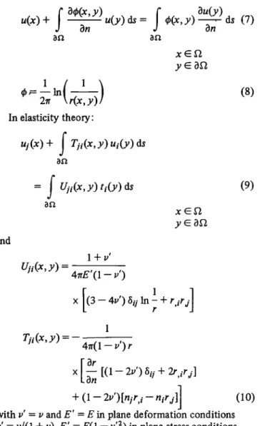
H(Xi) + (E<}>, Nu)sn = (Eu, N<t>)m (6) as a representational formula for u. In 2-D potential theory

J bn J on

an an

xGSl yGbCl

0 - — l n ( ) 2JT \r(x,y)/ In elasticity theory:

«,(*)+ j Tj,(x,y)u,0>)to

an

= J Uji(x,y)tj(y)ds an

(8)

(9) x G J 2

yGbQ.

and

uitQc,y) =

l + v'

TSi(x,y) =

-4TT£"(I - i/)

x [(3 - 4»') 8ff In ^ + rt /ry]

1 An{\ — v')r

x [ ^ [ ( l - 2 ^ ' ) 5/ / + 2r) Ir) /]

+ ( l - 2 i » ' ) [ n / ^ - n , ^ ] ] (10) with v' = v and £" = £• in plane deformation conditions

v' = i»/(l + v), E' = E(l — i/2) in plane stress conditions.

In order to reduce the equation to values defined at the boundary, a limiting process leads t o :

C(xi) u(xt) + (E4>, NU)M = (Eu, vV0)3n ₍₁₁₎

where C depends on the local boundary geometry.

The discretization of the previous equations as described elsewhere1 - 3 allows the establishment of a system of linear

equations whose solution produces the desired results. For instance, in potential theory and with an assumed linear evolution in £/as well as in bu/bn along the boundary (11), can be written as:

TV r 30(7) Vu(k) 1

an^

= I f WhN2)<t>k(l)dsk\

k=l J L anjt

'«*(*)

^a) «*(/) difc | "*; ' 1 (12)

qk{k + 1)J

where N stands for the number of elements into which the boundary has been discretized and Ni,N2 are linear

interpolation (shape) functions.

Nature o f t h e difficulty

Motz6 showed that near a corner of the interior angle a,

in a boundary where a continuous harmonic function u is defined, it is possible to represent it by a series:

1=1 a i=i «

( 0 < 6 < a ) (13) Where r, 6 are the local polar coordinates. When a>ir, the derivatives can be infinite when r -* 0.

In elasticity, the phenomenon is the same, and the stressed Oy can be factorized as:

otj = Go* (14)

where G is a function containing the singularity and (re-presents smooth behaviour.

As is seen, the nature of the singularity in both cases is similar. Different solutions have been presented to treat them. Jaswon and Symm7 have introduced an auxiliary

harmonic function; others8 use asymptotic analysis to

extrapolate experimental results; in other cases the mesh refinement is used, etc.

The following examples show some results when the singularity is of the type:

6 u-u0 + ar1'2 cos - + 0r 3/2

36

cos •

+ yrs

, 50 ' cos

f-2

(15)

which corresponds to a situation like that of Figure la. au

b6 •• r

1 / 2s i n - - -fir 3/2

3d

sin . 2

q 1 bu a . 0 3 30 - = = r , / 2s i n 0 r1 / 2s i n —

r bd 2 2 2 2 (16)

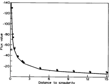
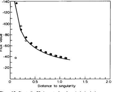
which derivative tends to infinity when r tends to zero. If a node of the discretization is situated on the singu-larity, the evolution of q near it resembles the curve shown in Figure lb.

The extrapolationprocedure consists of taking the smooth function q\/ras defined by values far enough from the singularity and their posterior identification with (16) in order to obtain the values of the coefficients in (16).

As an example of this method we present the problem (Figure 3) of the seepage under a sheet-pile, where the singularity appears at point A. The problem has been solved by superimposing a symmetric and a skew symmetric situation. Obviously the solution to the first one is a constant function; the skew symmetric case presents the factor r'1'2 around point A, being zero and the other

boundary conditions as shown in the figure.

Figure 4 depicts the discretization used in which a progressive mesh refinement near point A can be observed. The results are presented in Figure 5, where we have also plotted the solution obtained with the program BETIS;1 the

/ / / / s / / / .

O *1L ,q •dm

It

Figure 2

u av 4 .

o = 0

<7 = 0

Symmetric

Figure 3

0 = 0 0> = 0

( 7 = 0

Skew symmetric

1 5 m 1 8 m

1 8 m

Figure 4 Sheet-pile, 33 elements

-140

-120

-100-j>-80

6 9 Distance to singularity

12 15

Figure 5 Sheet-pile, 33 elements. ( ) analytical solution;

(+), asymptotic solution; (o), direct BIEM solution with BETIS program'

-40

o > X £-30

<k

°-20

1_

O 1-10

• •>»

^ » " s ^ _ ^

I I .____•

I I

•

I

6 9 12 Distance to singularity

), interpolation curve; 15

Figure 6 Sheet-pile, 33 elements. (

(+), solution with BETIS program1

curve corresponding to the exact solution for the full half-space is also plotted.

The intermediate results of the curve smoothed with y/r are shown in Figure 6. Figure 7 gives a table with the numerical values.

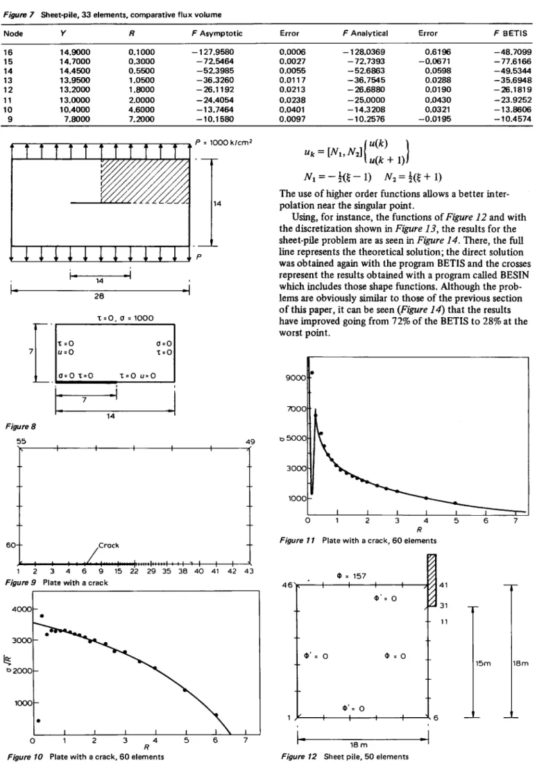
The second example of the same procedure is a square plate with a crack, supporting a traction of 1000 kg/cm2 (Figure 8). Due to the symmetry, it is only necessary to analyse a quarter of the plate under the conditions shown in Figure 8. The discretization can be seen in Figure 9, and in Figure 11 we have plotted the direct solution obrained using program SERBA2,3 with a full line as well as that obtained extrapolating the original function smoothed by \Jr. This regularized function has been represented in Figure 10, where it can be seen that the intensification

factor is Fc = 3587.09, which is only 0.91% in error with respect to the true solution.

Higher order interpolations

Node F Asymptotic Error F Analytical Error F BETIS

16 15 14 13 12 11 10 9

14.9000 14.7000 14.4500 13.9500 13.2000 13.0000 10.4000 7.8000

0.1000 0.3000 0.5500 1.0500 1.8000 2.0000 4.6000 7.2000

-127.9580 -72.5464 -52.3985 -36.3260 -26.1192 -24.4054 -13.7464 -10.1580

P = 1000 k/cm2

0.0006 0.0027 0.0055 0.0117 0.0213 0.0238 0.0401 0.0097

- 1 2 8 . 0 3 6 9 - 7 2 . 7 3 9 3 - 5 2 . 6 8 6 3 - 3 6 . 7 5 4 5 - 2 6 . 6 8 8 0 - 2 5 . 0 0 0 0 - 1 4 . 3 2 0 8 - 1 0 . 2 5 7 6

0.6196 - 0 . 0 6 7 1 0.0598 0.0288 0.0190 0.0430 0.0321 - 0 . 0 1 9 5

- 4 8 . 7 0 9 9 - 7 7 . 6 1 6 6 - 4 9 . 5 3 4 4 - 3 5 . 6 9 4 8 - 2 6 . 1 8 1 9 - 2 3 . 9 2 5 2 - 1 3 . 8 6 0 6 - 1 0 . 4 5 7 4

_E-I_

ISl

14

Figure 8

"*

=[

^

]

L

+

i))

J V i = - K * - l ) N2=fa+1) The use of higher order functions allows a better inter-polation near the singular point.

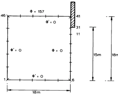
Using, for instance, the functions of Figure 12 and with the discretization shown in Figure 13, the results for the sheet-pile problem are as seen in Figure 14. There, the full line represents the theoretical solution; the direct solution was obtained again with the program BETIS and the crosses represent the results obtained with a program called BESIN which includes those shape functions. Although the prob-lems are obviously similar to those of the previous section of this paper, it can be seen (Figure 14) that the results have improved going from 72% of the BETIS to 28% at the worst point.

9 0 0 0

7 0 0 0

D5 0 0 0

3 0 0 0

1 0 0 0

-Figure 11 Plate w i t h a crack, 6 0 elements

4 6 V

1

X-* = 157 H 1 h

0 ' = 0

<(>'= o

0> = 0

J,

- 11

^ 6

15m 18m

Figure 10 Plate w i t h a crack, 6 0 elements

1 18 m

-140

-120

-100

Si-80

- 6 0

- 4 0

- 2 0

I i r J I I I l_ 0 5 1.0

Distance to singularity

1.5 2 0

Figure 13 Sheet-pile, 50 elements ( ), analytical solution;

(o), direct BIEM solution with BETIS program1; (+), special

function shapes (BESIN program)

This experiment encouraged us to implement singular elements, as can be seen in the following section.

Singular elements

As was said before, there exists the possibility of factorizing the natural variable in two parts: one with a smooth varia-tion and the other responsible for the infinite values near the singularity. If the last one is incorporated into the shape functions, the first will take on a finite value (the intensifi-cation factor) which can be perfectly managed by the computer. The idea then is nothing more than to interpolate qy/rin place of q near the singularity (Figure 16). Maintain-ing, for instance, the linear interpolation for q' = q\/r, it is possible to write:

q'Dk = (NhN2)\ ,

Wfc+i

or

but

QDk

\y/r \/r/yqk+1>

Qk= y/LkQk

and then:

M"^

;

3)ltJ

(17)

(18)

(19)

(20)

A6y

1 5 m 18m

1 8 m

Figure 15 Sheet-pile, 50 elements

which is the new interpolation rule for the singular element by the singularity.

It is clear that this idea can be used with every kind of interpolation and every order of the singularity. For instance, in the parabolic case:

«Ok=»?J^ *$J^

"J/VP-Qk

Qk+\

Vq'k

(21)

where N* are the current second degree shape functions with the midsize node.

According to Figure 16, the integrals to be evaluated are:

* - J £

h

Dk

B2= f — In (llr(x,y))N2 — dsk (22)

J 27T V

Dk

There are two cases that can appear depending on the relative position (inside or outside) of the singular element and the point from which the integration is done. The most important singularities are collected in the Appendix.

Taking the program BETIS1 as a basis, we have produced a new one, BENUM, which collects the singular elements. In Figures 16 and 17, some of the results comparing both solutions with the analytical one are given. As can be seen, the results are encouraging.

Figure 14 Sheet-pile, 50 elements, comparative flux value

Node 3 0 29 28 27 26 25 24 23 22 21 20 Y 14.9000 14.8000 14.7000 14.6000 14.5000 14.4000 14.3000 14.2000 14.1000 14.0000 13.9000 R 0.1000 0.2000 0.3000 0.4000 0.5000 0.6000 0.7000 0.8000 0.9000 1.0000 1.1000 F BESIN

- 9 1 . 4 9 5 6 - 1 1 0 . 4 9 6 3 - 7 3 . 8 8 6 7 - 6 4 . 5 5 6 2 - 5 6 . 5 8 9 6 - 5 1 . 0 8 5 2 - 4 6 . 7 9 1 8 - 4 3 . 3 4 9 9 - 4 0 . 5 0 1 3 - 3 8 . 0 9 1 3 - 3 6 . 0 1 5 3

Error

0.2854 - 0 . 2 3 0 4 - 0 . 0 1 5 8 - 0 . 0 3 2 9 - 0 . 0 2 0 2 - 0 . 0 1 6 6 - 0 . 0 1 3 3 - 0 . 0 1 1 1 - 0 . 0 0 9 3 - 0 . 0 0 7 8 - 0 . 0 0 6 5

F Analyt.

- 1 2 8 . 0 3 6 9 - 8 9 . 8 0 2 7 - 7 2 . 7 3 9 3 - 6 2 . 5 0 0 0 - 5 5 . 4 7 0 0 - 5 0 . 2 5 1 9 - 4 6 . 1 7 5 7 - 4 2 . 8 7 4 6 - 4 0 . 1 2 8 6 - 3 7 . 7 9 6 4 - 3 5 . 7 8 2 8

Error

0.7201 - 0 . 0 3 4 6 0.0691 0.0302 0.0264 0.0208 0.0175 0.01 51 0.0134 0.0122 - 0 . 0 4 3 4

F BETIS

0.5 1.0 1.5 2.0 Distance to singularity

Figure 16 Sheet-pile, 50 elements. ( ), analytical solution;

(o), direct BIEM solution with BETIS program'

Conclusions

The possibility of modelling the singular behaviour of the natural variables in plane problems by using special shape interpolation functions has been analysed.

The procedure can be implemented in elasticity as well as in potential theory and in every desired degree of accuracy with respect to the smooth part of the curve. Here we have presented the computations related to poten-tial theory with a linear -singular interpolation; a similar approach can be studied,7 in which the singularity has been incorporated into a constant element discretization for a plane elastodynamic steady-state case.

Appendix

The integrations which must be performed for the most representative cases in the section on singular elements are detailed below.

The singularity and the point where the integral equations is applied are on the same element

Two cases can be distinguished:

(1) The singularity and the integration point do not coincide {Figure A1)

Bi= J . V ( i n — )Ldr)

J V £ ( 1 - T ? ) \ Li?/

o

U v i - i ? J \/\-i\ J

where:

= -y/l[I1 + I2-I4\

/ i = | ——— lnZ,d77= f V Trr 7 l n Z , d i ? = l l n i .

J VI—V J

o o

It should be noted that when making the change 1 — TJ = t1,

we first check that this change of variable is correct.

0 <77 < 1 0 < 1 - T J < 1

?7 dr?

r T?dr?

J VT^~

1— V ,

= (-2) V I - T ? - — V T = 1 5

l - T J 1 - e

/ = lim —2 \J\— TJ Vl —f?

e-*o* 3

= 4/3

Therefore:

B2 = - y/Z [i In L - 0.370132]

(2) The singularity and the integration point coincide

(Figure A2)

r

Singularity < i Integration point

•n = 1 Tl = 0

Figure A1

-* Singularity = integration point

11 = 1

Figure A2

Tl = 0

Figure 17 Sheet-pile, 50 elements, comparative flux value

Node F B E N U M Error F Analyt. Error F BETIS

30 29 28 27 26 25 24 23 22 21 20

14.9000 14.8000 14.7000 14.6000 14.5000 14.4000 14.3000 14.2000 14.1000 14.0000 13.9000

0.1000 0.2000 0.3000 0.4000 0.5000 0.6000 0.7000 0.8000 0.9000 1.0000 1.1000

- 1 3 5 . 6 6 7 0 - 8 7 . 7 2 1 1 - 7 2 . 8 3 5 5 - 6 2 . 3 8 5 6 - 5 5 . 4 1 0 2 - 5 0 . 2 5 1 9 - 4 6 . 1 0 9 0 - 4 2 . 8 0 3 6 - 4 0 . 0 5 2 3 - 3 7 . 7 9 6 4 - 3 5 . 6 9 2 7

- 0 . 0 5 9 6 0.0232 - 0 . 0 0 1 3 0.0018 0.0011 - 0 . 0 0 0 0 0.0014 0.0017 0.0019 0.0000 0.0025

- 1 2 8 . 0 3 6 9 - 8 9 . 8 0 2 7 - 7 2 . 7 3 9 3 - 6 2 . 5 0 0 0 - 5 5 . 4 7 0 0 - 5 0 . 2 5 1 9 - 4 6 . 1 7 5 7 - 4 2 . 8 7 4 6 - 4 0 . 1 2 8 6 - 3 7 . 7 9 6 4 - 3 5 . 7 8 2 8

0.7201 - 0 . 0 3 4 6 0.0691 0.0302 0.0264 1.9792 0.0175 0.0151 0.0134 0.0122 0.0113

This integral can be expressed as:

1

'9'

B^j'-^lniULrftL&n

- * J ^

r- fn— l

= s/L lim —— In (IT?) dr? e~*o J vi?

6

We can fine a primitive function of:

7 ? - l

—— In (Z,r?) dr? VT?

integrating by parts: 17— 1

Vv

= (Ir?*2 - 2r?I/2) ln(Z,r?) - (|r?3'2 - 4r?1/2) Consdering that:

lim (ln/,T?)[|r?3/2-2T?1/2] = 0 r)-*0

which can easily be proved, as it can be written as °°/°° and therefore L'Hopital can be applied.

Therefore:

B^-y/LQkiL-%) Calculation of B2:

1

T? 1

•Ldrj

s/Lr\ Lrt

0 1

C v 1

B2=\ —=ln—,

J \fLr\ IT?

Proceeding in an analogous way to the calculation of B u we obtain:

5

= - v £ ( f l n Z , - i )

The singularity and the integration point are not on the same element

(1) The singularity lies to the left of the integration point.

r l \L

- 1

ngulanty

/• 1 1 - $ \L

% 2 rl

-ijl>

r~

where:

r=sjn-

and therefore :

dr Ls/r2-D2 d£ 2r Integrating by parts:

_ _ 1

- 1

-/a-

_]

- 1

#1 can be computed numerically through the following expression:

/ T 1 4

5

=

y-2

-

ln--X0-S)

G

1=1

where:

[LL r* nWi

2 2

Calculation of B2

~-1

n

- 1

V 2 J VT1 7! 2 \ r/2

- 1

integrating by parts:

j — 1

- 1

I (i-?)

(i + ? ) — r ^ - d ?

.a «4— • Singularity'

g=-1

Computing Z?2 numerically:

5

= f (l-*)

G,-£(l-$)

(l + »ffi

(2) The singularity lies to the right of the integration point (Figure A4)

r 1 \L 2?x= -7= ^ I n — d*

J y/r r 2

-J\\

2 J

2 r

- l

Integrating by parts and computing numerically:

i * i = I (l + t )1 / 2 Gi + 1 (l - 5X1 + £)1 / 2#i 1=1

Calculation o f 52: l

i = i

/• 1 1Z, B2= — 7 V2l n - - d |

J Vr 1-2

V 2 J VTTI 2 r

- l

Integrating again by parts:

j - i

B

=J^ [2V2 In i - f (1 + 5)

In ^ d|

- 1

1

+ J (l +

€)

'

\

<uj

Computing this numerically:

52

;

L 1 4

1=1

- 1

References

1 Paris, F. 'El Metodo de los Elementos de Contorno en la Teoria del Potencial y la Elasticidad'. Tesis Doctorla. E.T.S.I. Industriales de Marid, 1979

2 Alarc6n, E. et al. Comput. and Struct. 1979, 10, 351 3 Serba. 'A computer program for two dimensional elastostatics.

Advances in Engineering Software

4 Thompson, J. C. and Post, E. 'Asymptotic analysis techniques for for stress-concentration regions in plane problems'. Strain V 1977, 13 (4)

5 Jaswon and Symm. 'Integral equations methods in potential thoeory and elastostatic', Academic Press, London, 1977 6 AlarccSn, E. et al. 'Some minor problems with B.I.E.M'.

I Congr. Appl. Numer. Modelling. Madrid, 1978

7 Dominquez, J. and Alarc6n, E. 'Impedance of fundations using the boundary integral equation method'. Innovative Numerical Analysis for the Applied Engineering Sciences, Montreal, 1980 8 Brebbia, C. A. and Walker, S. 'Boundary element techniques in

engineering', Butterworth, London, 1979