Simplified methods for Next Generation IP Access Networks planning

Simplified methods for Next Generation IP Access Networks planning

ALBERTO E. GARCÍA, KLAUS D. HACKBARTH

Telematic Engineering Group GIT-DICOM University of Cantabria

Av. Los Castros sn, 39005 Santander – Cantabria SPAIN

http://www.tlmat.unican.es

Abstract: - The scope of this paper is to derive a set of simple formulas providing a traffic aggregation in

important points of an Internet access networks. The paper shows that the resources associated to the access network depend on user type-, technology and service parameter. Existing calculation methodologies applies on individual approximations whereas this proposal exposes the combined application of these individual and well-known approximations providing a scheme of generic dimensioning formulas. The dimensioning formulas for a generic applications are derived for the three main levels: connection, session and burst level, and the traffic aggregation is considered through three different and combined variables describing users, accesses and services forming a cube with three axes. The adaptation of corresponding parameters following the different axes allows the calculation of complete access network traffic scenarios, grouped by the so called CASUAL concept: Cube of Accesses / Services / Users. A set of CASUAL based tools allows an estimation of the aggregated traffic in different access points as multiplexers, IP point of presence or edge routers.

Key-Words: - traffic engineering, aggregation, access network, , architecture for Internet.

1 Introduction

The effect of the traffic aggregation has been broadly studied, usually under different approaches, to establish models and methods for carrying out estimations in form of corresponding parameters as mean value and variance. The solutions based on complex stochastic models use, for example markovian sources as MMPP - Modulated Makov Poisson Processes, associated with the main services supported by the network [1], [2]. Other solutions are based on simulation studies, considering both the sources and the networks elements [3]. Some statistical analysis over the network performance is even used in this type of studies, based on the knowledge acquired in the observation of the current Internet networks [4]. For the same purpose but following a different approach, there are some approximation methods as for example the "Network Calculus" [5], that allows obtaining solutions based on estimations carried out on the worst cases analyses of the network behaviour. This paper provides a comparison between two different methods and justifies their application inside an access network planning tool. The objective is to obtain the main parameters for aggregated Internet traffic resulting from different users and network access types and corresponding services.

2 Application of temporary scaled

behaviour of Internet traffic

Traditional methods of IP traffic characterization consider the protocols tower like an only queue system M/G/∞ [6] where the arrivals of request by session follow the classical Poisson model. But the characteristics of bursty traffics and the statistical parameters of the service utilization are very different to the telephony traffic and generate traffic traces with high autocorrelation values over long time observation. They are modelled using heavy tailed distribution functions.

Hence traffic in current IP networks does not provide a negative exponential distribution for the inter-arrival time, In fact the long term correlation of the IP traffic results an autocorrelation different from zero for increasing observation time which is completely opposite to the Poisson models. Taking into account the long term correlation behaviour, corrected Markov models have gone evolving from the self-similar pattern. Independently of the temporary period of observation the behaviour of these models is self-similar, showing autocorrelation figures that follow a clear hyperbolic decrease, see [7] and [8].

If the arrival process is approximated by a Poisson one but the service time duration is self similar the M/G/∞ model can be applied modelling the duration associated to the service process by a Pareto or Weibull distribution [9] because they provide a good approximation of the self-similar

nature of the global system. In function of the type of service associated to the modelling application, the use of heavy tails can be simplified including the classical case of the negative exponentials distribution as a special case; e.g. when VoIP traffic is included.

However, the use of the M/G/∞ is doubtful when the arrival process has to model self similar behaviour. This characteristic would imply the modelling of the traffic along the whole temporary scale, and not only at the level of calls, as in the case of the traditional markovian queue models. For this purpose we propose to use the different reference points that traditionally has been applied in the modelling of services of voice transmission, see [10] and [11], as a frame of reference for the modelling of different types of IP services.

Additionally we have to consider three time scales, as shown in figure 1:

‰ Connection level: This step models the

behaviour between two consecutive Internet accesses. Connection is considered similar as the call establishment to the Internet service provider over one of the access methods. The user-provider association usually impedes the establishment of multiple connections in a simultaneous way. Anyway there are some exceptions at high networks levels, e.g. bonding or bundling. The connection duration evolves with the access technology, the pricing scheme, the type of services and the socio-cultural situation in a particular way.

‰ Session level, considering as session, for

example, the download of an only Web page, a voice conversation, a videoconference, etc. This level models the time between two consecutive sessions inside a connection and the duration of each session. The concept of traffic aggregation can simplify the modelling of the multiservice scenario associated to the access to Internet by individual user. The characteristics of the traffic associated to a session depend on the type of service and application.

‰ Burst level, is the lowest reference level,

where the traffic patterns generated inside a session are modelled as the interarrival time of the objects or burst belonging to the service

3 Temporary Scaled On-Off

1

Model

The high difference of the time scale in the three temporal levels allows, from the point of view of the behaviour of the traffic generated by a source, to consider each temporary level as quasi-independent from the other. This results three two state sources hierarchically related where fig. 1 shows the inter-arrival time scale and fig. 2 the hierarchical relation.

Fig. 1: IP traffic interarrival temporary sequence

Fig. 2: Temporary scaled ON-OFF Model

At the connection level the ON-OFF source represents the connected or disconnected states, from the user to the ISP, 0 and 1 respectively. The fundamental parameters of the model are the time between connection requests and their corresponding durations.

At the session level the ON-OFF source represents the group of requests, transfers and the waiting times during each download, for example, of a web page. The first state, ‘0’ represents the periods of inactivity between sessions. The second state, ‘1’, models the group of requests and transfers associated to each session, voice communication, web page, ftp downloads, etc. The fundamental parameters of the model are the time between sessions and the duration of each session.

At the burst level the ON-OFF source models each one of the requests that compose each session. The states represent the idle time or latency between

1_{Really we use a generic two-states model. The}

classical ON-OFF model considers the OFF state as silence, Vmin=0, it is a singular case of generic

two-states model. Tb (between requests) Ton/off (between IP packets /objects) Burst Level Session Level Connection Level Ts (between connections) Tb (between requests) Ton/off (between IP packets /objects) Burst Level Session Level Connection Level Ts (between connections) 0 1 0 1 0 1 Connection Level Session Level Burst Level ISP disconnected Connected to ISP inactive Service Silence Transmit 0 1 0 0 11 0 1 0 0 11 0 1 0 0 11 Connection Level Session Level Burst Level ISP disconnected Connected to ISP inactive Service Silence Transmit

requests and the transfer of the objects associated to each request. In this case the fundamental parameters of the pattern are the time between requests and the time of service of associated to each request.

One of the advantages associated to this type of models is that when determining the bit rate associated to singular connection it is not necessary to know the number of transitions between each state (the number of transmitted objects) but only sojourn probability in one of the state. These values are determined starting from the average total sojourn time in each state.

2.1 Calculation

methods

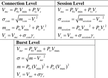
We can apply recursively the previous methodology along each temporary level obtaining in each case the associated traffic figures (the average rates corresponding to each level, and their variances). It is necessary to consider that the calculation of the rates associated to the connection level can be obtained knowing the activation and deactivation probabilities of the source (P1 and P0, corresponding to the ON_OFF states), and the typical deviation associated to this level (σcon), see Table I. However to obtain this values it is necessary to know the rates corresponding to the immediately inferior temporary level, this is the session level. In the same way, the statistical corresponding to the session level can only be obtained starting from the statistical of the inferior level.

Connection Level Session Level

0 min 1 mc c c s

V

=

P V

+

P V

2 con mcon Vc

σ

= − 2 2 0 min 1 con c c s

m

=

P V

+

P V

c mc con c

V

=

V

+

σ γ

0 min 1 ms s s r

V

=

P V

+

P V

2 session msession Vms

σ

= − 2 2 0 min 1 session s s r

m

=

P V

+

P V

s ms session s

V

=

V

+

σ

γ

Burst Level 0 min 1 max mr r r

V

=

P V

+

P V

2 mr m V

σ

= − 2 2 0r

(

min

)

1r

(

max

)

m

=

P V

+

P V

r mr r

V

=

V

+

σγ

Table I: Formulation of temporary scaled ON-OFF model

The Connection level provides the associated rate using the formulation corresponding to the considered ON-OFF source: the parameters corresponding to the activation probabilities is calculated by the mean sojourn times of the different

states, active or inactive, and the rates of data transmission associated to each state: the minimum rate (Vmin) in the inactivity event, and the total rate of the session level (Vs).

In the same way to the previous formulation, in the session level we could calculate the average rate using the corresponding ON-OFF source, and following the same process the burst level uses the corresponding ON-OFF model. However because inferior levels will no longer be contemplated, the rate of the burst activation period will take the value from the maximum rate of the connection, or the rate fixed by the group of protocols defined by the services. In this case Vmax is related with the rate of the burst, in some cases defined by the access bit rate.

2.2 Aggregation of temporary scaled

ON-OFF sources

The previous model describes only one source with one application but does not solve the problem of multi-sources providing a traffic mixture. Hence we have to consider the problem of the aggregation of independent sources must be solved. There are three approximations for the aggregated traffic calculation reference model: Statistical multiplexing, Markov Modulated based models and binomial approximations.

The Statistical Multiplexing approximation [12] calculates the equivalent capacity associated to N multiplexed sources as:

(

)

2 1 1 1 1 1 1

min

,

min

,

N N N i i i i i i N N N i i i i i i i i

C

a

R

a

R

R

ρ

σ

ρ

ρ

ρ

= = = = = =

⎧

⎫

⎪

⎪

=

_⎨

+

_⎬

⎪

⎪

⎩

⎭

⎧

⎫

⎪

⎪

=

_⎨

+

−

_⎬

⎪

⎪

⎩

⎭

∑

∑ ∑

∑

∑

∑

(1)

with ρi y σi2 as the average bit rate and its variance for the ith source, Ri is the maximum bit rate and, and a is a normalization factor depending of the error ε: a= −2ln

( )

ε

−ln 2

( )

π

(2)

The concrete case of modulated Markovian sources considers the superposition of N sources, and the maximum bound is calculated as

1 N i i

C

C

=

=

∑

(3)

with Ci as the equivalent capacity for the source i. Markov modulated based models, as for example shown in [13] as D-MMDP (Discrete-time Markov modulated deterministic process) model the on-off sources aggregation, using a discrete time Markov chain as modulator process. Following this idea, a D-MMDP system with (M+1) states defines an arrival

process with a bit rate controlled by the probability of two concurrent active sources which are calculated using a binomial function. However, the assumption of the Gaussian approximation (individual sources are normal and independent), the required bandwidth is calculated using the mean value and the variance of the aggregated traffic, as:

C

= +

µ σ

(

−

ln 2

( )

π

−

2ln

P

_l

)

(4)

with Pl as the loss probability. This is an approximation by an upper bound, based on maximum values, providing a loss-free estimation. On the contrary, the D-MMDP model uses an approximation based on effective bandwidth, but the results are similar.

4 Binomial approximation

The traffic mixture is usually carried out using a binomial distribution that models the aggregation; see [13] and [14]. The multiplexing of N independent On-Off sources is outlined in the figure 3.

Each source generates vp bits/sec in its active state. The aggregated data rate would be Nvp in the CBR source case. In case of the silence compression, one can profit from statistical multiplexing gain so that the needed server capacity C will be C = εvp with ε as the number of equivalent CBR sources. If k independent sources are active with probability pON, (N-k) sources are inactive with pOFF = (1-pON). Further there are (N over k) possibilities for choosing k elements out of N, see [15]. Thus the probability of k active sources follows a binomial distribution: In the mean E(k) = N*pON sources are active so the average data rate generated by N sources is E(v) = vp*N*pON. Therefore ε should satisfy the condition N ≥ ε > E(k) = N*pON.

If the server capacity is less than the potential maximum source data rate an overload condition can appear. Under this condition the server buffer will be filled and if no more buffer space is available packet loss occurs expressed by:

( ) (1 ) k N k k N k ON ON

N

N

Pk

p

p

k

k

α

β

α β α β

− −

⎛ ⎞

⎛ ⎞ ⎛

⎞ ⎛

⎞

=

_{⎜ ⎟}

⋅

⋅ −

=

_{⎜ ⎟ ⎜}

⋅

_{⎟ ⎜}

⋅

_⎟

+

+

⎝

⎠ ⎝

⎠

⎝ ⎠

⎝ ⎠

(5)

This can also be derived from the Markov chain of the M(N)/M/N binomial source model of figure 4. If the server provides capacity for N sources with su< ε < so all states from so to N cause overload and the overload probability is calculated as the probability

that they are more active sources than capacity is available: 1 ( ) (1 ) N i N i ol ON ON i C

N

P

P k C

p

p

i

− = +

⎛ ⎞

=

>

=

_{⎜ ⎟}

⋅

⋅ −

⎝ ⎠

∑

(6)

In (6) C expresses the server (=backbone) capacity in number of sources, k the number of active sources and N the total number of sources. Note that for pure loss systems without buffers the overload probability becomes the loss probability of the system. In the following we will assume a pure loss system.

α β vp vp E(v) = vp⋅N⋅pON α α β β C = vp⋅ε > E(v) 1 2 N source server buffer

Fig. 3: Multiplexing of On-Off sources

Fig. 4: M(N)/M/N state transition diagram To take into account loss probability as a function of pON and the number of sources N, the server capacity must be augmented by a correction value γ(PB,pON,N). This γ can be interpreted as a multiplier of the standard deviation of the aggregated data stream. The corresponding formulas are derived as follows: Total capacity for N aggregated binomial sources in bps: ( ) ( , , ) ( ) ( ( , , ) (1 )) B ON ON B ON ON ON p C E v P N p v N p P N p N p p v

γ

σ

γ

= + ⋅ = ⋅ + ⋅ ⋅ ⋅ − ⋅ (7)

Total number of equivalent circuits for N sources in vp units: ( ) ( , , ) ( ) ( , , ) (1 ) eq B ON p ON B ON ON ON C N E N P N p N v N p P N p N p p

γ

σ

γ

= = + ⋅ = ⋅ + ⋅ ⋅ ⋅ − (8)

Equivalent capacity for one binomial source in vp units: 0 1 _su so N-1 N Nα _α β soβ Nβ 2 (N-1)α 2β (N-su)α suv sov (N-1)v Nv 2v v

(1 ) ( , , ) eq eq CBR p ON ON ON B ON N C C v C v N N p p p P N p N γ = = = ⋅ ⋅ − = + ⋅ (9)

Limiting behavior of the equivalent capacity veq: N

lim

eq N

lim (

ON

)

ON

const

v

p

p

N

→∞

=

→∞

+

=

(10)

A binomial distribution is generally used to know the number of simultaneous occurrences of a group of independent statistical processes. However, in case of a bursty traffic nature, this aggregation is better modelled using a negative binomial distribution function.

This problem appears in the aggregation between the temporary levels. Evidently, the two lower levels (burst and session) requires in case of a service with bursty traffic nature to use a negative binomial based aggregation while services with independency between sessions and bursts needs to apply again a positive binomial distribution.

Bursty traffic means that when data are generated or received it is very probable that it continues to generate a quantity of data and when data generation is stopped it is very probable that the source continue to be in silence. The negative binomial distribution models this effect dividing the activation probability by the non activation probability. The result grows very quickly when the activation probability increase, simulating the continuation of the data arrival. Note that mostly the connection level is far of a bursty behaviour because a connection start indicates the invalidation of new calls (connections to the ISP are maintained during long periods, and only one by each user).

For this reason we used for the three levels a mixed model applying for the burst level a negative binominal and for the connection positive one. The distribution for the session level depends on the type of service, Table II resumes the formulas of both approaches where M is the number of independent processes (users in our case), N the total number of users, K the number of active users and P the activity probability.

Negative Binomial Function Classical Binomial Function

1 1

(1

)

k M k M M

P

P

+ − −

⎛

_{⎞⋅ ⋅ −}

⎜

⎟

⎝

⎠

*

*(1

)

N k N k k

P

P

−

⎛ ⎞

₋

⎜ ⎟

⎝ ⎠

2 [] * 1 var[] * (1 ) P Avg M P P M P = − = −

[]

*

*

[]

1

Avg

M P

M P

var

P

=

=

−

Table II: General Binomial Formulation

The mean number and variance of simultaneous active users N are:

1 1 1 2 1

*

1

[

]

*

(1

)

ms s ms

P

n

pop

P

P

v

var n

pop

P

=

−

=

=

−

(11)

Then the number of users transmitting a burst can be calculated by 2 2

(

* )*

1

mr ms s

P

n

n

v

P

γ

=

+

−

(12)

being Nmr the mean number of users transmitting a burst simultaneously, nms corresponds to the mean number of users with simultaneous active session, vs its variance for that level, and P2 indicates the probability of the active state of the burst. On the other hand, variance of the burst level users is expressed by:

[ ]

2 2 2 ( * )* (1 ) r mr ms s P v var n n v P γ = = + − (13)

with γ between 1 and 3.

For calculating the average number of users and their variance at the session level, in case of a binominal negative behaviour this method is applied in the same way providing the probabilities of the active states characteristic and the mean number and population's variance is given to the connection level. Once two lower time level are evaluated the connection populations can be calculated by the same methods as the two previous states, but using generally a positive binomial formulation. The rates are calculated starting from the averages of number of users and their variances:

2

*

var

[

]*

avg mr r avg mr r

V

n

v

V

var n

v

=

⎡

⎤ =

⎣

⎦

(14)

resulting the average value and the variance of the bit rate required by a user group for a certain service is calculated for a given group of users.

5 Network calculus based aggregation

aproximation

Analytical approximations obtain results with clear tendencies toward linearity, with simplifications represented by simple traffic figures. Network Calculus uses the simplification of generalist figures of traffic, limited bounds of real traffic, represented by arrival and service curves. The application of arrival curves and service curves represent generic approximations of the real behaviour of individual sources over different elements into the networks, see

[16]. Deterministic Network Calculus only considers the bounds corresponding to the most pessimistic cases, without consider the advantages associated to the statistical multiplexing of several flows over a single link. Statistical Network Calculus considers the Guarantees of Service characteristics for the aggregation of flows (deterministic service curve), and the individual guarantees (effective service curves).

An effective service curve represents the probabilistic bound for a service associated to a concrete flow. Using these curves allows establishing three possible approximations for the estimation of Guarantees of Service requirements:

1. Maximum bit rate estimation: If the service curve of each flow j shows the form

( )

t

P

t

S

j

=

j , we obtain the maximal bound

corresponding to the resources used by each flow j.

2. Mean bit rate estimation: The service curve of each flow j is

S

_j

( )

t

=

ρ

_j

t

, and now we could obtain the minimal bound for the resources used by each flow j. For example, the LBAP (Linear Bounded Arrival Processes) model, see [17], considers each traffic source like a token bucket

( )

b,

ρ

, with b its capacity and ρ the bit rate, with the arrival curve : A

( )

t ≤b+

ρ

t ∀t>0

3. Deterministic estimation: This method considers the best service curve accordingly with the resource reservation for each flow j assuring a concrete end to end delay.

The IETF defines a Guaranteed Service Class which assures a bandwidth without loss and with bounded maximum delay, see [18] and [19]. The associated traffic is called Tspec and it is modelled with two serialized token buckets. Their fundamental parameters are: Token bucket service rate r (bytes/sec), Capacity of the bucket b (bytes), Maximum bit rate p (bytes/sec), Maximum packet size M (bytes), and considering traffic control, the minimal unit of data m (bytes). This model establishes very clear bounds for the end to end delay. This is the reason because the Tspec definition can be generalised to characterise traffic sources with concrete behaviours related with the different Internet services. For example, the Guaranteed Service traffic is characterised by an arrival curve with the Tspec parameters: Tspec(r, b, p, M) with the expression: a t

( )

=min

(

M+ pt b, +rt

)

(15)

In the same way, the service curve is calculated as

( )

₌

(

₋

)

+

V

t

R

t

c

, with

D

R

C

V

=

+

and R as the service rate. C and D depend of the processing type (e.g. PGPS: C=M and D=M’/c, with M as the maximal size of packets, M’ the MTU and c the link bitrate).

Accordingly with this behaviour, the required reserved capacity for a determined path (assuring a maximum delay dmax) is calculated as:

max max b M p M C p r p R r b M d D R p r M C R p r d D − ⎧ _{+ +} ⎪ ₋ ≥ ≥ ⎪ ₋ ⎪ _{+ −} = ⎨ ₋ ⎪ + ⎪ _{≥ ≥} ⎪ ₋ ⎩ (16)

This approximation has he following limitation; it is only applicable into the concrete aggregation points. In these points, the nodes have proportional resources accordingly to the number of connected sources. Moreover maintaining the low delay criteria supposes the necessity of a lot of resources, and then, the aggregation of individual sources increases the over dimensioning of the aggregated traffic estimation. Applying this methodology into the aggregation points (into the access network POP or including at the backbone edge), several TSPEC sources can be grouped following the RFC 2212 and RFC 2216 indications. Addition of N TSPEC flows generates a new TSPEC flow with the expression:

(

)

( )

1 1 1 1 , , , , , , max n i i i i i n n n i i i i i i i TSpec r b p M TSpec r b p M = = = = ⎛ ⎞ = _{⎜ ⎟} ⎝ ⎠

∑

∑ ∑ ∑

(17)

This function shows the addition of N input flows and it allows dimensioning the system with a shared reservation of resources, but in some cases, the result could be higher than the smallest sum.

Applying the Network Calculus, the exact sum for each flow associated to each Tspec could be calculated, and its value will be less or equal than the Summed Tspec, as figure 5 shows. The calculation uses the concatenation of (N+1) token buckets to obtain the arrival curve for the set of N flows (represented by the ⊗ operator of Network Calculus), called Cascaded-Tspec, resulting a Tspec curve with the form:

(

)

(

)

1 1 1 1 1 1 1 , , , n k k j l l l j k l l n k k j l l l j k l l p r b M M TSpec p r b M M = + = = − − = = = ⎛ ⎞ + − + ⎜ ⎟ ⎜ ⎟ ⎜ ⎟ + − + ⎜ ⎟ ⎝ ⎠

∑

∑ ∑

∑

∑ ∑

(18)

Fig. 5: Comparison between real and approximate calculations based on T-Spec based methodology.

6 Application of the traffic aggregation

calculation in the planning of the access

network

The application of these methodologies allows simplifying many of the procedures related with the network planning and dimensioning. For this purpose the GIT (Group of Telematic Engineering) of the University of Cantabria has developed a tool denominated CASUAL (Cube of Accesses / Services / Users of Free Assignment) incorporating these models and calculation schemes. We apply these models for the dimensioning of the capacities in fixed and mobile access networks under the concept of a traffic scenario resulting from the user’s connection commonly to an access network point.

The CASUAL tool serves as a generator of scenarios for modelling aggregated INTERNET accesses traffic considering each access network like a group of services, directly related with the type of users, and the type of access architecture. Under this scheme a scenario results a graphically representation in form of a cube by means of three axes (access type, type of user, type of service). The application carries out the modelling of each service individually, accordingly with the user's characteristics and the access type, completing each one of the individual cubes following the three main axes:

1. Axis “users”: The different behaviour of the users, although the idea is quite subjective, it can be defined in a relative way to the likeness of customs and necessities related in a certain group of clients. These likenesses are even clearer when behaviours associated with certain economic and labour status are observed.

2. Axis “accesses”: The different access configurations and types of physical media to use, each one with different characteristic, as capacities and market penetration.

3. Axis “services”: Today the Internet world is populated by an enormous number of services, and even the parameter of the existing services are in a continuous change. Hence a service definition with a generic set of parameters is required.

We observed that most of current and future services can be modelled with the approach shown in this paper and changes in its characteristics can be mapped into corresponding variations in some of their parameters. Modelling each sub-cube, CASUAL carries out the estimation of the traffic associated to each one of these subcubes, so that it is possible to establish the fundamental parameters, and to outline the appropriate aggregation approaches to the related aggregation point.

Fig. 6: Three dimensional concept of 3G-IP scenarios definition

Following this classification the corresponding arrival curves are determined, being able to be associated to concrete scheduling mechanisms, and therefore to dimension the aggregation point (for example a multiplexer or an "Edge Router").

Each axis could be used to obtain an aggregated traffic figure, accordingly to their individual associated parameters. Following each separated axis

Web MODEM PYME Web MODEM SOHO Video ISDN SOHO Web ISDN Residential Web MODEM Residential Voice MODEM Residential Video MODEM Residential

is possible to obtain statistical approaches related to the aggregated traffic, for example, by user’s groups, individual users or typical services. Combined utilisation of binomial approximation and TSpec Calculus method allows obtaining the final aggregated traffic associated to complete access network scenarios.

7 Conclusion

This paper exposes a new application of traditional calculation methods which are combined to model the complex Internet traffic behaviour. The proposal uses a generalization of the ON-OFF model with three time scales as simplification of self-similar traffic behaviour. Calculations are simpified with binomial approximations and service characterization follows the Network Calculus principles to obtain corresponding arrival curves. The resulting methodology allows the generation of multiples scenarios of IP access networks, considering customer characterization, services and access types. An example of this implementation type is called CASUAL-TAROCA-IP, developed by GIT/DICOM of Cantabria University. This tool serves as entrance source for tools specialized in the design and dimensioning of a 3G Internet backbone network.

References:

[1] Dolzer, Payer: “A simulation study on traffic aggregation in Multiservice Network” Proceedings of the IEEE Conference on High

Performance Switching and Routing (ATM 2000),

pp. 157-165, Heidelberg, 2000

[2] Y. Serbest, San-qi Li: “Unified Measurement Functions for Traffic Aggregation and Link Capacity Assessment”, IEEE Infocom '99:The

Conference on Computer Communications,

Volume 3, pp. 1522-1531, 1999.

[3] D. Clark, W. Lehr: “Provisioning for Bursty Internet Traffic: Implications for Industry and Internet Structure”, MIT Press, 2001

[4] T. Ferrari: “End to end performance analysis with traffic aggregation”, Computer Networks Journal, Vol. 34, nº6, pp. 905-914, Amsterdam, 1999 [5] J. Y. LeBoudec, P. Thiran: “Network Calculus: A

theory of deterministic Queuing Systems for the Internet”. Ed. Springer Verlag LNCS 2050. July 2002

[6] Peter Pieda. “The dynamics of TCP and UDP interconnection in IP-QoS differentiated services networks”. Nortel Networks

[7] W. E. Leland, M. S. Taqq, W. Willinger, and D. V. Wilson, "On the self-similar nature of {Ethernet} traffic," presented at ACM SIGCOMM

Conference on Communications Architectures,

San Francisco, California, 1993.

[8] R. J. Mondragon, D. K. Arrowsmith, J. M. Griffiths, and J. M. Pitts, "Chaotic Maps for Network Control: Traffic Modelling and Queuing Performance Analysis," Performance Evaluation, vol. 43, pp. 223-240, 2001.

[9] V. Paxson, S. Floyd. “Wide area traffic: the

failure of Poisson Modelling”. Lawrence Berkeley

lab.

[10] N. X. Liu and J. S. Baras, "Long-Run Performance Analysis of a Multi-Scale TCP Traffic Model," IEE Proceedings

Communications, vol. 151, pp. 251-257, 2004.

[11] A. Riedl, M. Perske, T. Bauschert, and A. Probst, "Dimensioning of IP Access Networks with Elastic Traffic," presented at Networks 2000, Toronto, Canada, 2000.

[12] Wang, S., Zheng, H. and Copeland, J.A., Video Multiplexing with QoS Constraints. in

IEEE SPIE Conference on Internet Routing and QoS, (1998), 81-91.

[13] Ni, J., Yang, T. and Tsang, D.H.K. Source Modelling, Queuing Analysis and Bandwidth Allocation for VBR MPEG-2 Video Traffic in ATM Networks. IEE Proceedings on

Communications, 143 (4). 197-205.

[14] R. Parkinson, "Traffic Engineering

Techniques in Telecommunications," vol. 2005:

Infotel System Corporation, 2002.

[15] A. E. Garcia, K. D. Hackbarth, A. Brand, R. Lehnert: "Analytical Model for Voice over IP traffic characterization", WSEAS Transactions on

Communications, vol. 1, pp. 59-65, 2002.

[16] J. Liebeherr, S. Patek, and A. Burchard, "A Calculus for End-to-End Statistical Service Guarantees," University of Virginia, Charlottesville, USA CS-2001-19, June 2001 2001.

[17] R. G. Garroppo, S. Giordano, S. Niccolini, and F. Russo, "DiffServ Aggregation Strategies of Real Time Services in a WF2Q+ Schedulers Network," Lecture Notes in Computer Sciences, vol. 2170, pp. 481-491, 2001.

[18] J. Schmitt, M. Karsten, and R. Steinmetz, "Aggregation of Guaranteed Service Flows," presented at 7th IEEE/IFIP International

Workshop on Quality of Service (IWQoS'99),

London, UK, 1999.

[19] J. Schmitt, M. Karsten, and R. Steinmetz, "On the Aggregation of Deterministic Service Flows," Computer Communications, vol. 24, pp. 2-18, 2001.