Obesity and socio-economic inequalities in spain: evidence from the ECHP

(1)

Obesity and socio-economic inequalities in spain: evidence

from the ECHP

David Cantarero Marta Pascual

University of Cantabria (Spain) University of Cantabria (Spain)

Abstract

This paper explores the relationship between obesity, measured by the Body Mass Index (BMI), and socio-demographic characteristics in Spain. Empirical work is based on data from the European Community Household Panel (ECHP). The results obtained through probit models show that factors such as age, education, marital status, health status and some economic data are relevant in explaining whether an individual is obese or not.

This work has been partially supported by the Ministerio de Educación y Ciencia (SEJ2004-02810) and the Spanish Institute of Fiscal Studies. The authors would like to thank anonymous referees and the editor for helpful suggestions. The usual disclaimer applies.

Citation: Cantarero, David and Marta Pascual, (2007) "Obesity and socio-economic inequalities in spain: evidence from the

ECHP." Economics Bulletin, Vol. 9, No. 3 pp. 1-9

Submitted: December 18, 2006. Accepted: January 31, 2007.

(2)

1

1. INTRODUCTION

Being overweight or obese is one of the most significant health issues facing developed countries. However, obesity is not only a significant risk factor for some diseases (including coronary heart disease, diabetes, hypertension, sleep apnea, cancer, etc.) but also has important economic consequences (higher health expenditure, lower productivity, lower earnings, etc.). A review of the literature enables us to verify that there exists evidence about the impact of obesity on health status (Nayga 1997), on earnings (Baum and Ford 2004), on economic activity (Hamermesh and Biddle 1994) and on occupation selection (Morris 2006). Thus, the purpose of this paper is to analyse which socio-economic variables (gender, age, education, income, etc.) are related with the increasing prevalence of obesity in Spain. The analysis is conducted using microdata from the European Community Household Panel and the structure of the paper is as follows. Section 2 describes the data set and the variables involved in the analysis. In Section 3, empirical results based on probit models are presented. Finally, concluding remarks are shown in Section 4.

2. DATA AND METHODOLOGICAL DECISIONS: THE ECHP

The data used in this paper come from the European Community Household Panel (ECHP). This survey contains data on individuals and households for the European Union countries with eight waves available (1994-2001). The main advantage is that information is homogeneous among countries since the questionnaire is similar across them. However, only from 1998 to 2001 there is available information about individuals’ weight and height in Spain.

In order to measure body fat, we have used as indicator the Body Mass Index (BMI) which uses a height-weight relationship to calculate individual’s ideal weight. BMI has become the medical standard used to measure overweight and obesity. It is calculated as weight in kilograms divided by height in meters squared. Thus, individuals with BMI over 25 kg/m2 are overweight and individuals with BMI ≥ 30 kg/m2 are classified as obese. TABLE I reports mean BMI for each year. It can be also noted that from 1998 to 2001 this indicator shows that Spanish population has overweight problems.

TABLE I

Summary Statistics of BMI Distribution. Country: Spain.

1998 1999 2000 2001 Mean 25.17 25.19 25.14 25.38 Std. Deviation 4.22 4.19 4.12 4.33 Minimum 13.67 11.56 11.11 11.72 Maximum 63.69 63.61 60.97 66.41 Number of Observations 12598 12014 11502 11712

(3)

2

3. THE MODEL AND EMPIRICAL RESULTS

The objective of this paper is to deep in the relationship between obesity and socio-demographic characteristics. Our dependent variable in the statistical model is a dichotomy variable which takes a value of 1 if the individual has a BMI over 25 Kg/m2 and 0 otherwise. In this way, the respondent is overweight (Y=1) or not (Y=0) in the corresponding period. A set of factors, such as age, marital status, education, etc., gathered in a vector x explain this fact so that: ). , ( 1 ) 0 ( Prob ), , ( ) 1 ( Prob β β x F Y x F Y − = = = = (1)

The set of parameters β reflects the impact of changes in x on the probability. In order to estimate this equation, a nonlinear specification of F(.) can prevent logical inconsistency and the possibility of predicted probabilities outside the range [0,1]. The most common nonlinear parametric specifications are logit and probit models which have been analysed. So, we will use a latent variable interpretation (Jones 2001). Let

0 0 0 1 ≤ = > = * i * i y if y y if y (2) where ε β + = ' * x y . (3)

If we assume that ε has a standard normal distribution, we obtain the probit model, while assuming a standard logistic distribution, we obtain the logit model. These models are usually estimated by maximum likelihood estimation and the log-likelihood for a sample of independent observations is:

[

]

{

}

∑

= − − + = 1 ' ' ) ( 1 ln ) 1 ( ) ( ln ln i i i i i F x y F x y L β β . (4)

In order to establish the main socio-demographic characteristics of obesity, we have classified them into eight groups of variables: personal and household characteristics, education level, marital status, income, occupational status, variables related to individuals’ health, social relationships and lifestyles. TABLE II shows explanatory variables used in estimations and their corresponding definitions.

Firstly, as personal characteristics we have included two variables: individual’s age (in years) and gender (building a dummy variable which takes value of 1 if individual is MALE and 0 otherwise). To allow for a flexible relationship between the SAH and AGE, a quadratic polynomial function of this variable is included (AGE2=Age2).

The second group of variables are referred to the maximum level of education completed. In the ECHP, education is classified into three categories based on ISCED classification: less than secondary level (ISCED 0-2), second stage of secondary level (ISCED 3) and third level (ISCED 5-7). Thus, a dummy variable has been included: third level education (HIGHEDUC).

(4)

3

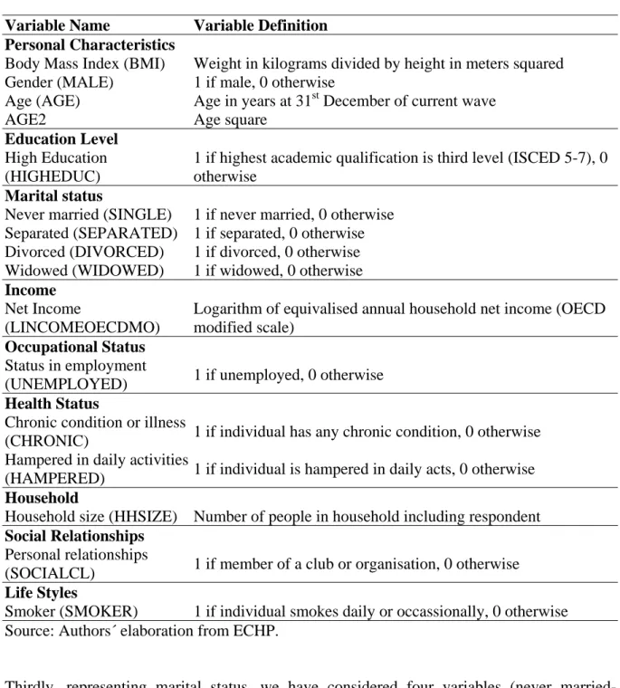
TABLE II

Variables Definitions

Variable Name Variable Definition

Personal Characteristics

Body Mass Index (BMI) Weight in kilograms divided by height in meters squared

Gender (MALE) 1 if male, 0 otherwise

Age (AGE) Age in years at 31st December of current wave

AGE2 Age square

Education Level

High Education (HIGHEDUC)

1 if highest academic qualification is third level (ISCED 5-7), 0 otherwise

Marital status

Never married (SINGLE) 1 if never married, 0 otherwise Separated (SEPARATED) 1 if separated, 0 otherwise

Divorced (DIVORCED) 1 if divorced, 0 otherwise

Widowed (WIDOWED) 1 if widowed, 0 otherwise

Income

Net Income

(LINCOMEOECDMO)

Logarithm of equivalised annual household net income (OECD modified scale)

Occupational Status

Status in employment

(UNEMPLOYED) 1 if unemployed, 0 otherwise

Health Status

Chronic condition or illness

(CHRONIC) 1 if individual has any chronic condition, 0 otherwise

Hampered in daily activities

(HAMPERED) 1 if individual is hampered in daily acts, 0 otherwise

Household

Household size (HHSIZE) Number of people in household including respondent

Social Relationships

Personal relationships

(SOCIALCL) 1 if member of a club or organisation, 0 otherwise

Life Styles

Smoker (SMOKER) 1 if individual smokes daily or occassionally, 0 otherwise

Source: Authors´ elaboration from ECHP.

Thirdly, representing marital status, we have considered four variables (never married-SINGLE, SEPARATED, DIVORCED and WIDOWED) with married as the reference category.

On the other hand, we are concerned with the influence of income on obesity. Our income variable is equivalised annual net household income (LINCOMEOECDMO) adjusted using OECD modified scale to take into account household size and composition.

The income measure is disposable (after tax) individual income. However, the reference period of income is the year prior to interview and the interviews corresponding to the first eight waves of the ECHP were performed from 1994 to 2001, meaning that the corresponding incomes refer, respectively, from 1993 to 2000 (eight years). Nevertheless, as we are

(5)

4

interested in combining individuals’ characteristics with households’ income, we will focus on the information corresponding to 2000.

Other variables included in the analysis related to occupational status are status in employment. We have considered a dummy variable that takes value one if the individual is unemployed and zero otherwise (UNEMPLOYED).Also, we have considered other variables related to health status. For example, we have taken into account if an individual has any chronic condition (CHRONIC) or is hampered in daily acts (HAMPERED).

Finally, we have considered number of people in household including respondents (Household size-HHSIZE). Also, another dummy variable has been built in order to take into consideration whether an individual is a member of a club or organisation or not (SOCIALCL). As well, we have incorporated another dummy variable which takes value 1 if individual smokes daily or occasionally (SMOKER). TABLE III reports the results of the estimation

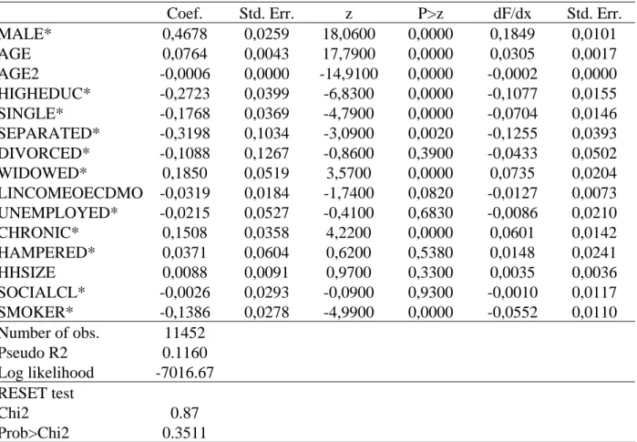
TABLE III

Probit Estimates including average and marginal effects.

Dependent variable: Binary variable which takes value one if an individual is overweight or obese.

Coef. Std. Err. z P>z dF/dx Std. Err.

MALE* 0,4678 0,0259 18,0600 0,0000 0,1849 0,0101 AGE 0,0764 0,0043 17,7900 0,0000 0,0305 0,0017 AGE2 -0,0006 0,0000 -14,9100 0,0000 -0,0002 0,0000 HIGHEDUC* -0,2723 0,0399 -6,8300 0,0000 -0,1077 0,0155 SINGLE* -0,1768 0,0369 -4,7900 0,0000 -0,0704 0,0146 SEPARATED* -0,3198 0,1034 -3,0900 0,0020 -0,1255 0,0393 DIVORCED* -0,1088 0,1267 -0,8600 0,3900 -0,0433 0,0502 WIDOWED* 0,1850 0,0519 3,5700 0,0000 0,0735 0,0204 LINCOMEOECDMO -0,0319 0,0184 -1,7400 0,0820 -0,0127 0,0073 UNEMPLOYED* -0,0215 0,0527 -0,4100 0,6830 -0,0086 0,0210 CHRONIC* 0,1508 0,0358 4,2200 0,0000 0,0601 0,0142 HAMPERED* 0,0371 0,0604 0,6200 0,5380 0,0148 0,0241 HHSIZE 0,0088 0,0091 0,9700 0,3300 0,0035 0,0036 SOCIALCL* -0,0026 0,0293 -0,0900 0,9300 -0,0010 0,0117 SMOKER* -0,1386 0,0278 -4,9900 0,0000 -0,0552 0,0110 Number of obs. 11452 Pseudo R2 0.1160 Log likelihood -7016.67 RESET test Chi2 0.87 Prob>Chi2 0.3511

(*) dF/dx is for discrete change of dummy variable from 0 to 1. z and P>|z| are the test of the underlying coefficient being 0.

(6)

5

The sign of the coefficients inform us about the qualitative effect of the explanatory variables. In this way, if the sign of the coefficient on MALE is positive, this means that men are more likely to be overweight or obese relative to the reference individual who are women. Estimates show that most of the coefficients are significant and have the expected signs. Individuals who are more likely to be overweight are men with low level of education and income. Also, we observe a positive relationship between being overweight and being hampered in daily activities. As well, if an individual smokes or is a member of a club or organisation is less likely to be overweight. An average, the probability of male individuals being overweight is 0.1849 more than for female individuals. TABLE III also shows the RESET test for the probit model concluding that there is no evidence of mis-specification. The chi-squared test statistic is 0.87 with a p-value well above conventional significance levels (p=0.3511)

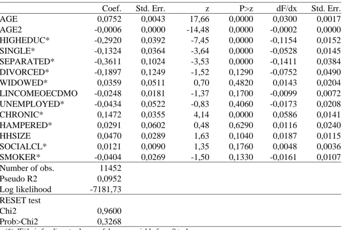
Finally, to test the sensitivity of our results, subsets of individuals aggregated by gender have been constructed. The categories to be analysed are overall, females and males. TABLES IV, V and VI report the results obtained. Thus, we can observe small differences. Widowed women are more likely to be overweight while widowed men are more likely. Also, males who are hampered in daily activities are less likely to be overweight or obese than women.

TABLE IV

Dependent variable: Binary variable which takes value one if an individual is overweight or obese. Category: Overall.

AGE 0,0752 0,0043 17,66 0,0000 0,0300 0,0017 AGE2 -0,0006 0,0000 -14,48 0,0000 -0,0002 0,0000 HIGHEDUC* -0,2920 0,0392 -7,45 0,0000 -0,1154 0,0152 SINGLE* -0,1324 0,0364 -3,64 0,0000 -0,0528 0,0145 SEPARATED* -0,3611 0,1024 -3,53 0,0000 -0,1411 0,0384 DIVORCED* -0,1897 0,1249 -1,52 0,1290 -0,0752 0,0490 WIDOWED* 0,0359 0,0511 0,70 0,4820 0,0143 0,0204 LINCOMEOECDMO -0,0248 0,0181 -1,37 0,1700 -0,0099 0,0072 UNEMPLOYED* -0,0434 0,0522 -0,83 0,4060 -0,0173 0,0208 CHRONIC* 0,1472 0,0355 4,14 0,0000 0,0586 0,0141 HAMPERED* 0,0291 0,0602 0,48 0,6290 0,0116 0,0240 HHSIZE 0,0470 0,0289 1,63 0,1040 0,0187 0,0115 SOCIALCL* 0,0121 0,0090 1,35 0,1760 0,0048 0,0036 SMOKER* -0,0404 0,0269 -1,50 0,1330 -0,0161 0,0107 Number of obs. 11452 Pseudo R2 0,0952 Log likelihood -7181,73 RESET test Chi2 0,9600 Prob>Chi2 0,3268

(7)

6

TABLE V

Dependent variable: Binary variable which takes value one if an individual is overweight or obese. Category: Males.

AGE 0,0875 0,0062 14,04 0,0000 0,0342 0,0024 AGE2 -0,0008 0,0001 -12,88 0,0000 -0,0003 0,0000 HIGHEDUC* -0,1986 0,0567 -3,50 0,0000 -0,0785 0,0226 SINGLE* -0,2710 0,0523 -5,18 0,0000 -0,1065 0,0206 SEPARATED* -0,4511 0,1577 -2,86 0,0040 -0,1784 0,0610 DIVORCED* -0,0227 0,2262 -0,10 0,9200 -0,0089 0,0889 WIDOWED* -0,0378 0,1049 -0,36 0,7180 -0,0148 0,0413 LINCOMEOECDMO 0,0061 0,0267 0,23 0,8210 0,0024 0,0105 UNEMPLOYED* -0,1332 0,0759 -1,76 0,0790 -0,0526 0,0302 CHRONIC* 0,0498 0,0528 0,94 0,3460 0,0194 0,0205 HAMPERED* -0,0129 0,0921 -0,14 0,8880 -0,0051 0,0361 HHSIZE 0,0182 0,0398 0,46 0,6480 0,0071 0,0155 SOCIALCL* -0,0146 0,0131 -1,12 0,2630 -0,0057 0,0051 SMOKER* -0,1397 0,0370 -3,78 0,0000 -0,0547 0,0145 Number of obs. 5509 Pseudo R2 0,0939 Log likelihood -3403,55

(8)

7

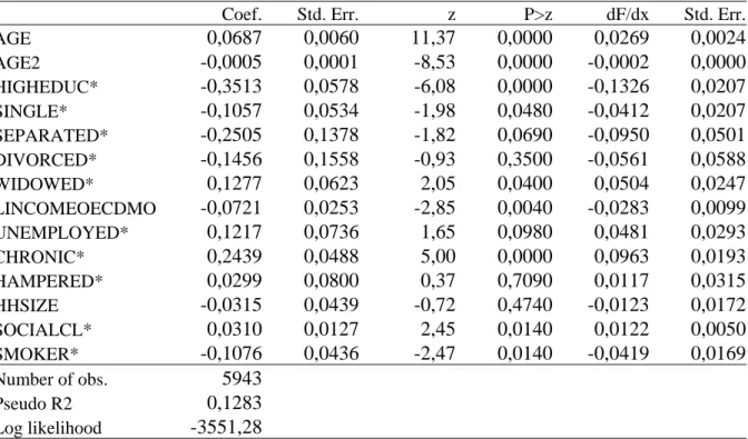
TABLE VI

Dependent variable: Binary variable which takes value one if an individual is overweight or obese. Category: Females.

AGE 0,0687 0,0060 11,37 0,0000 0,0269 0,0024 AGE2 -0,0005 0,0001 -8,53 0,0000 -0,0002 0,0000 HIGHEDUC* -0,3513 0,0578 -6,08 0,0000 -0,1326 0,0207 SINGLE* -0,1057 0,0534 -1,98 0,0480 -0,0412 0,0207 SEPARATED* -0,2505 0,1378 -1,82 0,0690 -0,0950 0,0501 DIVORCED* -0,1456 0,1558 -0,93 0,3500 -0,0561 0,0588 WIDOWED* 0,1277 0,0623 2,05 0,0400 0,0504 0,0247 LINCOMEOECDMO -0,0721 0,0253 -2,85 0,0040 -0,0283 0,0099 UNEMPLOYED* 0,1217 0,0736 1,65 0,0980 0,0481 0,0293 CHRONIC* 0,2439 0,0488 5,00 0,0000 0,0963 0,0193 HAMPERED* 0,0299 0,0800 0,37 0,7090 0,0117 0,0315 HHSIZE -0,0315 0,0439 -0,72 0,4740 -0,0123 0,0172 SOCIALCL* 0,0310 0,0127 2,45 0,0140 0,0122 0,0050 SMOKER* -0,1076 0,0436 -2,47 0,0140 -0,0419 0,0169 Number of obs. 5943 Pseudo R2 0,1283 Log likelihood -3551,28

SOURCE: Own elaboration from ECHP (2000 and 2001).

4. CONCLUSIONS

The prevalence of obesity in modern societies has risen considerably since last years specially among children. Obviously, obesity is a multi-factor problem which is affected by genetics, diet, lifestyles, physical activity and environment. However, there exist socio-economic characteristics which are related with obesity. The results obtained provide new evidence about the relationship between the increasing prevalence of obesity in Spain and socio-demographic characteristics (gender, age, education, income, etc.). Empirically, we have used the new information contained in the ECHP.

In this study, it is interested in seeing if socio-economic variables have different effects of men and women taken as separate classes. We can conclude that obesity is more prevalent in males with low levels of education and not married. Also, obesity is positively related with those chronic illnesses which hampered female’s activities. This is an important result to take into consideration to elaborate effective policies to fight against obesity in modern societies.

(9)

8

5. REFERENCES

Baum, C.L., Ford, W.F. (2004) “The Wage Effects of Obesity: A Longitudinal Study”

Health Economics, 13, 885-899.

Hamermesh, D.S., Biddle, J.E. (1994) “Beauty and the Labor Market” The American

Economic Review, 84(5), 1174-1194.

Jones, A.M. (2001) Applied econometrics for health economists-A practical guide, Office of Health Economics, Whitehall London.

Morris, S. (2006) “Body Mass Index and Occupational Attainment” Journal of Health

Economics, 25, 2, 347-364.

Nayga Jr, R.M. (1997) “Obesity and Heart Disease Awareness: A Note on the Impact of Consumer Characteristics Using Qualitative Choice Analysis” Applied Economics Letters, 4, 4, 229-231.