DIFFERENCES IN THE ECONOMIC GROWTH OF LATIN AMERICAN COUNTRIES. INTEGRATION EFFECTS AND FOREIGN DIRECT INVESTMENT INFLUENCE.

(1)

REVISTA INVESTIGACIÓN OPERACIONAL Vol., 29 No 1, 10- 25, 2008

DIFFERENCES IN THE ECONOMIC GROWTH OF

LATIN AMERICAN COUNTRIES. INTEGRATION

EFFECTS AND FOREIGN DIRECT INVESTMENT

INFLUENCE.

Marta Bengoa, Ana M. Carrera and Adolfo C. Fernández1 Department of Economics. University of Cantabria.

ABSTRACT:

This paper tries to explain the wide range of economic experiences among Latin American countries taking into account the role of capital formation and foreign direct investment (FDI) as a drive engine of growth. We design a model in which FDI generates endogenous, non zero growth. In particular, FDI brings about growth because it facilitates the entry of intermediate goods of more advanced technology in the host country. In contrast, if the entrance of FDI is obstructed or precluded by policy measures in the host country, the growth rate of the latter will be smaller or even zero. Integration enables countries to exchange more varieties of goods and eases technological diffusion through FDI. The predictions are tested empirically using GMM technique in a panel data performed by 18 Latin American countries over the period 1970-2000. The estimations suggest that Latin America’s growth rates are positively related to a more open attitude and to a greater integration in international markets. However, the empirical analysis also points out to the need of a certain degree of social capacity to ensure a successful integration. Finally, the empirical exercise confirms the positive connection between FDI and growth predicted by the model.

RESUMEN

El objetivo del presente trabajo es doble: en primer lugar, desarrollar un modelo de crecimiento endógeno que analice la influencia de la inversión extranjera directa en el crecimiento del PIB per cápita en términos reales de una economía en desarrollo; y, en segundo lugar, contrastar de forma empírica si la inversión extranjera ha contribuido al crecimiento del producto en América Latina teniendo en cuenta las diferencias entre países. Con este fin, se desarrolla un modelo de crecimiento endógeno que se aplica a dos escenarios: una economía abierta que permite la entrada de capitales foráneos y una economía cerrada que no autoriza la entrada de tales capitales. El crecimiento es mayor en el primero de los escenarios, y su motor es la inversión extranjera, que coexiste con el capital local. En el análisis empírico se utiliza la metodología de datos de panel con el fin de estudiar el efecto de la IDE en el crecimiento económico latinoamericano durante el periodo 1970-2000, y se explora en qué medida una mayor libertad económica y un entorno institucional adecuado han contribuido al crecimiento económico de América Latina.

KEY WORDS: Endogenous growth, less developed countries, panel data estimation. MSC 91B62 JEL F43- O11-O41.

1 INTRODUCTION

The abundant research on economic growth that has flourished from the mid 80s onwards has underlined the role of endogenous technological progress as one of the main drive engines of growth (Romer, 1990; Grossman and Helpan, 1991; Aghion and Howitt, 1992). However, the potential access to inventions and new designs is not homogeneous among countries. As the literature has also pointed out, some countries are capable to innovate and produce their own technology. Other, instead, may lack the necessary skills to generate new discoveries and implement them in the productive process. These countries, usually Less Developed Countries (LDCs), will have to benefit from the diffusion of the technology that is produced elsewhere.

In the last decades the literature has stressed a particular channel whereby technology may spill over from advanced to laggard countries, allowing the latter to grow at higher rates (Grossman and Helpman, 1991; Romer, 1994; Jones, 1995; Barro and Sala-i-Martín, 1997; Aghion and Howitt, 1998): i.e. the entrance of Foreign Direct Investment (FDI). This point of view vividly contrasts with the common belief that was accepted in some academic and political spheres in the

1_{Corresponding author Department of Economics, University of Cantabria, Av. Los Castros s/n 39005} Santander (Spain), Pone 34-942 20 20 05 Fax 34-942 201603; Email [email protected]

(2)

1950s and 60s, according to which FDI was deleterious for the economic performance of LDC. Fortunately, the theoretical discussion that permeated part of the development economics of the second half of the 20th_{century has been} approached from a new angle on the light of the New Growth Theory. Thus, the models built in this novel framework provide an interesting background in order to study the correlation between FDI and the growth rate of GDP. This literature has developed various hypotheses that explain why FDI may potentially enhance the growth rate of per capita income in the host country. First, FDI is one of the main transmission vehicles of advanced technology from leaders to developing countries (Borensztein, De Gregorio and Lee, 1998).

In addition, FDI may ease the exploitation and distribution of raw materials that are produced in the host country, by means of helping improve the network of transport and communication. FDI may also have a positive impact on the productive efficiency of domestic enterprises. Finally, FDI may also raise the quality of domestic human capital and improve the know-how and managerial skills of local firms, that have an opportunity to increase their efficiency by learning from and interacting with foreign firms (the so called learning by watching effect).

On empirical grounds, some recent contributions have detected a positive connection between FDI and growth. De Gregorio (1992) finds a positive and significant impact of FDI on economic growth in a panel of 12 Latin American countries over the period 1950-1985. Blomström, Lipsey and Zejan (1992) pursue a cross-country analysis of a sample of 78 developing countries. They report that the (positive) impact of FDI on growth is larger in those countries that exhibit higher levels of per capita income. Balasubramanyan et al. (1996) reach to the same result for export promoted countries. Borensztein, De Gregorio and Lee (1998) suggest that FDI enhances economic growth by means of easing technological diffusion. This effect is detected in a set of 69 LDC over the years 1970-89. They also report a higher impact of FDI on growth than that of domestic investment. Balasubramanyam, Salisu and Sapsford (1996) employ a cross-country procedure to analyze 46 LDC in 1970-85. Their results suggest that FDI enhances growth in those cases in which the host country has adopted trade liberalization policies. Zhang (2001) documents a similar result. De Mello (1999) employs time series and panel data analysis over a sample of both OECD and non-OECD countries in the years 1970-1990. He claims that FDI has a positive impact on growth if there is complementarily between foreign and domestic investment. Bengoa and Sánchez-Robles (2003) explore the correlation between FDI and economic growth in Latin America, over the period 1970-2000. They find also a positive and significant impact of FDI on the economic growth of the countries of this area.

The first part of this paper is devoted to design and discuss a model intended to provide some theoretical background to these (and other related) empirical results. The model is inspired in those designed by Romer (1990), Grossman and Helpman (1991), Rebelo (1991), Barro and Sala-i-Martín (1995) and Borensztein, De Gregorio and Lee (1998). It is first presented in an open economy setting. Later on in this paper we shall discuss the closed economy version of the model, in order to compare the predictions suggested by both models regarding the rate of growth of the economy. Finally, we perform an empirical test of the model using data from a sample made up by 18 Latin American countries over the years 1970-2000.

2. THE MODEL IN AN OPEN ECONOMY.

The main features of the model in an open economy scenario are the following:

1. Total production in the economy is elaborated taking as inputs the stock of capital in the host country (or domestic capital) together with the capital accumulated from the foreign direct investment in the country.

2. Since the model is mainly designed for a developing country, it seems reasonable to assume that capital mobility is imperfect due, for example, to the existence of capital controls. This restriction entails that agents cannot convert local assets in foreign currency at the official rate, or that there are limits to this exchange. Similarly, it could be assumed that the country gets funds from abroad to finance just one part of its stock of capital, whereas the rest (the domestic component) is financed with local savings (Barro, Mankiw and Sala-i-Martín, 1995). Capital controls will create a wedge between domestic and international interest rates, and therefore the model will consider two different interest rates.

3. Foreign firms operating in the country produce capital goods xi, where i indexes the ith variety of intermediate good. The entrance of new firms endows the domestic economy with new varieties of

intermediate goods.

4. Technical progress in the model is linked to the entry of new sorts of capital goods that in turn increase the stock of domestic capital. These goods will typically embed more advanced technology in them.

(3)

2.1.1. Preferences.

The economy is populated by individual agents with standard Ramsey (1928) preferences. The utility function is thus of the form

∫

∞ −

=

0

)

(

)

0 (

e

u

c

L

dt

u

ρt _t _t

σ

−

=

−

1

1 )

(

1 t

c

u

₍₁₎

Where ρ is the rate of time preference, ct per capita consumption at time t and Lt the size of the family. There is only one consumption good in the economy. Population remains constant for simplicity. The utility function is of the CRRA form, where σ is the inverse of the intertemporal elasticity of substitution.

2.1.2. Technology and the decision to invest.

The economy thus described produces the final consumption good Y, which will be sold in competitive markets. The production function of Y is of the form

Yt= A Ktα α β − =

⎥

_⎦

⎤

⎢

⎣

⎡

∑

1 , 1 FDI t N i it

x

0<α<1; 0<β<1 (2) where A is exogenous and constant by assumption, and it captures not only the state of technology stricto sensu but also other aspects related with the efficiency in the economy as, for example, the institutional framework (Basu and Weil, 1998). In other words, and following the terminology of Abramovitz (1986) “A” is a proxy of the social capacity of the host economy.

The stock of domestic capital is represented by K. The capital brought in by foreign firms is denoted by FDI, and is composed by Nt, FDI (notice that NFDI is a continuous function with finite derivatives) varieties of intermediate capital goods, each one of them denoted by xi. α and β are the elasticities of output with respect to K and xi correspondingly. From now on, we shall omit the subscript t in order to alleviate notation.

Intermediate goods enter in an additive and separate form into the production function. This means that they are neither perfect substitutes nor perfect complements. In contrast to other models (Grossman and Helpman, 1991; Aghion and Howitt, 1992), the entrance of new varieties of durables does not render the existing intermediate goods obsolete. The production function described by equation (2) exhibits decreasing returns in each intermediate good, and also in the total number of these goods, NFDI. It will be shown below that this point is crucial for foreign firms to decide whether to invest or not into the country. Finally, the production function exhibits constant returns to scale in K and NFDI considered together.

Let us assume that a foreign firm is trying to decide whether to undertake an investment project in this country or not. The firm will invest in this country as long as the rate of return of a new variety of intermediate goods (plus the cost associated to the entrance in the country) exceeds the interest rate prevailing in the international market rw_.

We can think of this entry cost as the payment of fees, legal procedures, paperwork, and other outlays entailed by the adaptation of the managers of the firms to the local environment.

The entry cost will be assumed to be a percentage φ of the profits of the firm. It will typically depend on the attitude of the host country to the entrance of new firms. More formally, a new firm will entry into the local economy if the productivity of the new project net of the entry cost exceeds the world interest rate (equation 3):

(1-φ) FDI

N

y

∂

> rw ₍₃₎

(4)

(1-φ) A Kα_(1-α) _x α β − =

⎥

_⎦

⎤

⎢

⎣

⎡

∑

FDI t N i it

x

, 1 iβ > rw (4)

If condition (4) is fulfilled, new firms will come into this country, therefore increasing the number of available varieties of capital goods. The increase in NFDI, in turn, decreases the marginal productivity of new varieties of capital until the point in which the marginal productivity of a new type of good (net of the entry cost) equals the world interest rate. Notice that this assumption is necessary in order to prevent a massive entry of foreign firms in the local economy.

In equilibrium:

(1-φ) A Kα_(1-α) −α _x

FDI

N

β(1-α)_{= r}w ₍₅₎ The increase in the number of intermediate goods will also bring about an increase in the stock of domestic capital2_{, and hence foreign and domestic capital will grow at the same pace.}

Technological progress is captured by an increase in the number of available varieties of intermediate goods. This feature of the model implies that FDI is the channel whereby the host country can access state of the art technology.

A further assumption that shall be made concerns the dynamics of domestic capital. The law of motion of domestic capital has the standard form

K

c

Y

K

=

−

δ

• (6) where a dot over a variable represents its derivative with respect to time, and δ is the depreciation rate in the economy.

2.2. Discussion of the model.

The final good Y is made up by the combination of A, domestic capital and the different varieties of intermediate goods. It is sold in competitive markets at a price normalized to 1 for simplicity. It is irrelevant whether Y is produced by local or foreign firms. In this model, however, the production of the intermediate good is carried out by foreign firms.

We shall assume that each firm produces a single variety of the intermediate good xi in a monopolistic competition setting, and sells or rents the good to final producers at the price Pi. The demand function for each variety of intermediate good can be obtained by means of equating Pi to the marginal productivity of xi in the production of the final good.

Pi = A Kα (1- α) 1 (7) 1 − − =

⎥⎦

⎤

⎢⎣

⎡

_∑

β α β

β

_i FDI N i i

x

Pi= A β (1- α) Kα −α _x FDI

N

iβ(1-α)-1 (7´) The foreign firm sells the good at the price Pi, and faces a (constant) marginal cost that will be normalized to 1. The firm will choose the price and the quantity produced of xi in order to maximize profits (8) in each point of time:

ΠiFDI= (Pi – 1)xi (8)

We can plug the expression of Pi as given by (7´). The optimization problem for the firm is3:

2_{Intuitively, a new firm that settles down in the host country to provide, for example, phone facilities, will require the support of}

domestic capital (offices, machines to construct the network, and so forth) thus contributing to the increase of domestic K.

(5)

Max

[A β (1- α) K i x α −α _x FDI

N

iβ(1-α)-1– 1] xi dt (9) The optimal quantity of the ith_{good is thus:}

xi =x*₌

[

β

(

−

α

)

α −α

]

1−β(1−α) 1 2 2

1 K

N

_FDI

A

(10)

The optimal quantity of the intermediate good is positively related to A, K, α and β. Plugging (10) in (7’) yields the complete expression for the monopoly price:

Pi= A β (1- α) Kα α − FDI

N

[

(

)

]

β( α) α β α α

α

β

− − − − −

−

2 (1 ) 11 1 2

1 K

N

_FDI

A

(11) P=

₍

₎

α

β

1 −

1

(12)

The quantity and the monopoly price are the same for all xi since the marginal cost is equal for all xi, and every good enters the production function in the same way4_{. Using the fact that intermediate goods are} independent among them, the production function can be written as:

Y= A Kα

N

_FDI1−α

x

_iβ(1−α) (13)

Notice that the production function is homogeneous of degree 1 in N and K, and therefore the model behaves like an AK model.

As shown above, the equilibrium condition that warrants the entrance of FDI in the host economy is: (1-φ) A Kα_(1-α) −α _x

FDI

N

iβ(1-α) = rw

It is necessary to take into account that in any time the world interest rate will fulfill the following equation: rw_{= (1-φ) (1-α)} FDI

N

Y

(14) NFDI is thus: NFDI= (1-φ) (1-α) _w

r

Y

(15)

Replacing the expression in (15) for NFDI into (13) yields

K

x

A

Y

_i α α β(1 )

~

−

=

(16) where

(

)(

)

α α α

α

φ

−

⎥⎦

⎤

⎢⎣

⎡

−

≡

1 1

1

1 ~

w

r

A

(17)

4_{This kind of symmetry is a property common in the models that resemble the contributions by Romer (1990) and Barro and}

(6)

2.3. Steady State Growth.

In order to close the model we must make explicit the behavior of individuals. The maximization problem of the consumers can be written as:

Max Ut =

e

dt

c

t ρt σ

σ

− ∞ −

∫

₋

−

0 1

1

(18) subject to

K

=

Y

−

c

−

δ

K

•

If we add the initial condition K0>0 this problem can be solved by standard optimal control techniques. The Hamiltonian is:

H = e-ρt

c

t

λ

(

Y

c

δ

K

)

σ

−

+

⎟⎟

⎠

⎞

⎜⎜

⎝

⎛

−

1

1 (19) Where λ is the shadow price of domestic capital. The first order conditions and the transversality condition are as follows: Hc=0 e-ρt c-σ-λ=0 (20) -Hk=

λ

&

λ

&

= -

λ

(

MgPK

−

δ

)

(21) Where

K

Y

MgPK

∂

=

0 =

∞ → t t t

K

lim

λ

(22)

Taking logs and derivatives with respect to time and plugging in the resulting expression in (21) yields an equation for the rate of growth of the economy, c (23).

(

ρ

δ

)

σ

γ

=

MgPK

−

c

1

(23) For the particular case of the production function described in (16), the rate of growth can be written as:

( )

⎟

⎠

⎞

⎜

⎝

⎛

₋

=

−

ρ

δ

σ

γ

α α β1 *

1 ~

i

x

A

(24)

Expressed in terms of the parameters of the model (see Appendix 1):

(

)

⎥

⎦

⎤

⎢

⎣

⎡

−

=

β

α

₋+

φ

−

ρ

δ

σ

γ

α 2ηβ _ηη₍₁(1_ββ₎ ) η(1 β) 1 *

1

1 (

1 )

w

r

A

(25) where

α

η

=

1 −

(7)

1. The combination of FDI and the stock of domestic capital warrants the existence of positive and endogenous rates of growth in the host country. Moreover, FDI provides the host country with more advanced intermediate goods, thus acting as a channel whereby technology generated in more advanced countries may be adopted in laggard nations.

2. The rate of growth in the economy is inversely related to the opportunity cost of investing in international capital markets (rw_{). Thus, higher world interest rates will disincentives flows of direct} investment among countries, hence reducing the rate of growth in LDCs.

3. The rate of growth is also negatively correlated with the cost that the foreign firm has to pay in the host country. Economic policy may thus influence the amount of inflows coming into the country by means of altering this cost. The parameter will be lower in outward oriented countries, which remove regulations to the entrance of FDI and ease the paperwork necessary for foreign firms to settle down into the country. The attraction of FDI will be encouraged and the economy will be able to grow at faster rates. Inward oriented countries, instead, will exhibit higher values of ; they will be less appealing to FDI as a potential destiny and therefore will grow at a slower pace.

3. THE MODEL IN A CLOSED ECONOMY.

For the sake of comparison we shall present the model in a closed economy set up. To come closer to the model described above we shall assume that there is an initial stock of FDI (although this assumption is not crucial). In contrast to above, however, now policymakers are reluctant to allow new inflows of FDI into the country, and therefore NFDI is constant over time.

The production function is similar as the one discussed for the open economy:

Yt= A Ktα α β − =

⎥

_⎦

⎤

⎢

⎣

⎡

∑

1 , 1 FDI t N i it

x

0<α<1; 0<β<1 (26)

Since foreign investment is constant, the production function can be written as:

Yt=

BK

_tα (27)

where

B

=

AN

_FDI1−α. The law of motion of capital is again:

K

=

Y

−

c

−

δ

K

•

The agents face the same maximization problem. It is straightforward to show that the rate of growth is

(

α

ρ

δ

σ

γ

*

₌

1

α−1

₋

K

B

)

(28)

Replacing B by its value we get the rate of growth of the economy:

(

α

ρ

δ

σ

γ

*

₌

1

1−α α−1

₋

K

N

A

_FDI

)

(29)

Since FDI is taken as constant and the production function is concave in K, the model now mimics the Ramsey model. The economy will eventually achieve a steady state with no growth.

4. EMPIRICAL RESULTS

Next, we have pursued an empirical exercise in order to test the connection between FDI and growth. The data have been obtained from the standard sources in the growth literature (the Summers-Heston data basis, IMF and World Bank). We have chosen a sample of 18 Latin

(8)

American countries5_{, over the years 1970-2000. Since the model is designed basically for countries that} imitate technology, it made sense to us to focus on a set of nations that have the following features: they are developing countries (and therefore most likely to be imitators rather than innovators), they have a certain level of social capacity that allows their profiting form the entrance of FDI, and they have had different trajectories in terms of growth. We think that the Latin American countries share these features.

Finally, while there are already a number of papers that explore the impact of FDI on developing countries, the number of articles that deal explicitly with Latin America is still insufficient, in our view.

Table 1. FDI and growth in Latin America (1970-2000). Estimation in levels.

LEVELS

Number of firms: 18 Sample period is 1970 to 2000 Observations: 108 Degrees of freedom: 101 Dependent variable is: growth

RSS = 0.047606 TSS = 0.068456 Estimated sigma-squared (levels) = 0.000471

Wald test of joint significance: 6.028928 df = 1 p = 0.014 Wald test - jt sig of time dums: 36.526099 df = 5 p = 0.000 Wald test selected by user: 6.028928 df = 1 p = 0.014 Testing: fdi

Variable Coefficient Std. Error T-Statistic P-Value CONST 0.020037 0.005423 3.694689 0.000220 fdi 0.437400 0.178139 2.455388 0.014073 D71 -0.008451 0.007246 -1.166295 0.243495 D72 -0.037511 0.007255 -5.170611 0.000000 D73 -0.025255 0.007237 -3.489734 0.000484 D74 0.009652 0.007339 1.315179 0.188450 D75 0.024895 0.008817 2.823600 0.004749 Test for first-order serial correlation: 3.248 [ 18 ] p = 0.001 Test for second-order serial correlation: 1.683 [ 18 ] p = 0.092

LEVELS

Instruments used are:

CONST nothing TIM DUMS

Variable Coefficient Std. Error T-Statistic P-Value CONST -0.044001 0.029541 -1.489492 0.136358 fdi 0.447341 0.194667 2.297986 0.021563 rate -0.105129 0.047735 -2.202365 0.027640 D71 -0.010750 0.006736 -1.596022 0.110484 D72 -0.042125 0.005234 -8.048149 0.000000 D73 -0.032037 0.008281 -3.868916 0.000109 D74 0.018284 0.007943 2.301712 0.021351 D75 0.035029 0.007255 4.828287 0.000001 Test for first-order serial correlation: 2.065 [ 18 ] p = 0.039 Test for second-order serial correlation: 1.644 [ 18 ] p = 0.100

Software: DPD98 for Gauss, Arellano and Bond (1998). Standard errors and test statistics robust to heteroskedasticity.

5_{The countries that encompass the sample are Argentina, Bolivia, Brazil, Chile, Colombia, Costa Rica, R. Dominican,} Ecuador, El Salvador, Guatemala, Honduras, Mexico, Nicaragua, Panama, Paraguay, Peru, Uruguay and Venezuela.

(9)

We have estimated a simplified version of equation, approximating the various variables and parameters by the most similar available (24). The dependent variable is the rate of growth, computed over five year’s averages, in order to depurate the data from the influence of the business cycle. The regressors are:

a) FDI (in percentage of GDP). We have not included local investment to avoid collinearity with FDI (the data available of local investment compiled by standard sources, as the IMF, already include the flows of FDI)

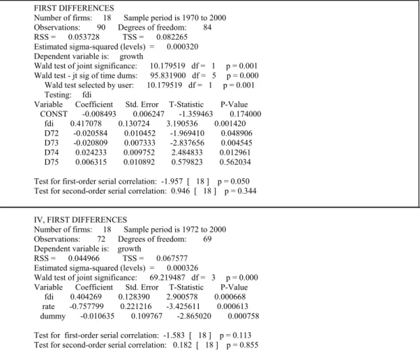
Table 2. FDI and growth in Latin America (1970-2000). Estimation in first differences.

FIRST DIFFERENCES

Number of firms: 18 Sample period is 1970 to 2000 Observations: 90 Degrees of freedom: 84 RSS = 0.053728 TSS = 0.082265 Estimated sigma-squared (levels) = 0.000320 Dependent variable is: growth

Variable Coefficient Std. Error T-Statistic P-Value CONST -0.008493 0.006247 -1.359463 0.174000 fdi 0.417078 0.130724 3.190536 0.001420 D72 -0.020584 0.010452 -1.969410 0.048906 D73 -0.020809 0.007333 -2.837656 0.004545 D74 0.024233 0.009752 2.484833 0.012961 D75 0.006315 0.010892 0.579823 0.562034 Test for first-order serial correlation: -1.957 [ 18 ] p = 0.050 Test for second-order serial correlation: 0.946 [ 18 ] p = 0.344

IV, FIRST DIFFERENCES

RSS = 0.044966 TSS = 0.067577 Estimated sigma-squared (levels) = 0.000326

Wald test of joint significance: 69.219487 df = 3 p = 0.000 Variable Coefficient Std. Error T-Statistic P-Value fdi 0.404269 0.128390 2.900578 0.000668 rate -0.757799 0.221216 -3.425611 0.000613 dummy -0.010635 0.109767 -2.865020 0.000758 Test for first-order serial correlation: -1.583 [ 18 ] p = 0.113 Test for second-order serial correlation: 0.182 [ 18 ] p = 0.855

Software: DPD98 for Gauss, Arellano and Bond (1998). Standard errors and test statistics robust to heteroskedasticity. b) The level of efficiency in the economy A has been captured indirectly by several proxies. The black market premium (bm) is a measure of the degree of distortions in local markets and it is a variable frequently used as a proxy for the integration effects (see Sachs and Warner, 1997; Rodriguez and Rodrik, 1999). Therefore larger values of the black market premium will entail lower levels of efficiency. The same can be said of the ratio of public consumption to GDP (con): a high value of this indicator will generally mean that the degree of intervention of the public sector in the economy is larger, and inputs’ productivity will be lower. Inflation (infl) is usually associated with a larger degree of regulations in the economy or with a lack of commitment of the monetary authority to preserve economic stability. On a priori grounds, then, it will entail lower efficiency of the correspondent country. Ile is the index of economic freedom of the Fraser Institute. Larger values of the index entail less regulated markets and higher levels of efficiency and growth. Two variables are included to capture the potential impact of human capital, which most theoretical studies associate to higher levels of efficiency in the economy: the percentage of enrollment at the secondary level (secun) and the percentage of enrollment at the primary level (prima).

(10)

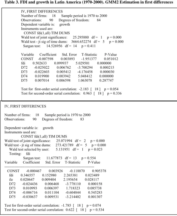
Table 3. FDI and growth in Latin America (1970-2000). GMM2 Estimation in first differences

CONST fdi(1,all) TIM DUMS

Wald test of joint significance: 25.295880 df = 1 p = 0.000 Wald test - jt sig of time dums: 3664.652274 df = 5 p = 0.000 Sargan test: 14.526956 df = 14 p = 0.411

Variable Coefficient Std. Error T-Statistic P-Value CONST -0.007598 0.003893 -1.951377 0.051012 fdi 0.502633 0.099937 5.029501 0.000000 D72 -0.025022 0.006762 -3.700294 0.000215 D73 -0.022603 0.005412 -4.176458 0.000030 D74 0.019900 0.003942 5.048412 0.000000 D75 0.007014 0.006598 1.063078 0.287747

Test for first-order serial correlation: -2.183 [ 18 ] p = 0.054 Test for second-order serial correlation: 0.963 [ 18 ] p = 0.336

Sargan test: 11.677873 df = 13 p = 0.554 Variable Coefficient Std. Error T-Statistic P-Value --- CONST -0.000467 0.003926 -0.118870 0.905378 fdi 0.346557 0.152980 2.265381 0.023489 ile 0.020647 0.009404 2.195654 0.028117 D72 -0.024436 0.006468 -3.778110 0.000158 D73 0.010993 0.006397 1.718323 0.085738 D74 -0.006716 0.011104 -0.604844 0.545283 D75 -0.030637 0.009531 -3.214402 0.001307 Test for first-order serial correlation: -1.785 [ 18 ] p = 0.074 Test for second-order serial correlation: 0.622 [ 18 ] p = 0.534

c) The world interest rate has been proxied by the Federal Reserve Bank three months treasury bill rate.

d) Finally, we have included several time dummies for each of the five subperiods. D71 corresponds to 1975-80, D72 to 1980-85, D73 to 1985-90, D74 to 1990-95 and G75 to 1995-2000

Table 1 displays the results obtained by estimating our baseline specification by OLS in levels. We already observe that FDI is positively and significantly correlated with economic growth. In the first part of the table the point estimate for FDI is 0.43 and the t-statistic associated to this parameter is 2.45. Time dummies are negative for the years 75-80, 80-85 and 85-90 and positive for the rest of the period. This result makes sense since in the mid 70s and the 80s Latin America suffered the negative impact of the debt crises, whereas the 90s envisaged a remarkable recuperation.

In the second part of Table 1 we have included the world interest rate. As predicted by our model, the correlation with growth is negative. The point estimate is significant. Intuitively, higher world interest rates disincentive the flows of FDI to LDC and thus entail lower rates of growth.

(11)

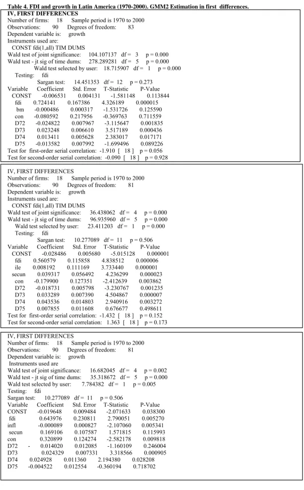
Table 4. FDI and growth in Latin America (1970-2000). GMM2 Estimation in first differences. IV, FIRST DIFFERENCES

Wald test of joint significance: 104.107137 df = 3 p = 0.000 Wald test - jt sig of time dums: 278.289281 df = 5 p = 0.000

Wald test selected by user: 18.715907 df = 1 p = 0.000 Testing: fdi

Sargan test: 14.451353 df = 12 p = 0.273 Variable Coefficient Std. Error T-Statistic P-Value CONST -0.006531 0.004131 -1.581148 0.113844 fdi 0.724141 0.167386 4.326189 0.000015 bm -0.000486 0.000317 -1.531726 0.125590 con -0.080592 0.217956 -0.369763 0.711559 D72 -0.024822 0.007967 -3.115647 0.001835 D73 0.023248 0.006610 3.517189 0.000436 D74 0.013411 0.005628 2.383017 0.017171 D75 -0.013582 0.007992 -1.699496 0.089226 Test for first-order serial correlation: -1.910 [ 18 ] p = 0.056 Test for second-order serial correlation: -0.090 [ 18 ] p = 0.928 IV, FIRST DIFFERENCES

Sargan test: 10.277089 df = 11 p = 0.506 Variable Coefficient Std. Error T-Statistic P-Value CONST -0.028486 0.005680 -5.015128 0.000001 fdi 0.560579 0.115858 4.838512 0.000006 ile 0.008192 0.111169 3.733440 0.000001 secun 0.039317 0.056492 4.236299 0.000023 con -0.179900 0.127351 -2.412639 0.003862 D72 -0.018731 0.005798 -3.230767 0.001235 D73 0.033289 0.007390 4.504867 0.000007 D74 0.043536 0.014803 2.940916 0.003272 D75 0.007855 0.011608 0.676677 0.498611 Test for first-order serial correlation: -1.432 [ 18 ] p = 0.152 Test for second-order serial correlation: 1.363 [ 18 ] p = 0.173 IV, FIRST DIFFERENCES

Number of firms: 18 Sample period is 1970 to 2000 Observations: 90 Degrees of freedom: 81 Dependent variable is: growth Instruments used are

Wald test of joint significance: 16.682045 df = 4 p = 0.002

Wald test - jt sig of time dums: 35.318672 df = 5 p = 0.000 Wald test selected by user: 7.784382 df = 1 p = 0.005

Testing: fdi . Sargan test: 10.277089 df = 11 p = 0.506

Variable Coefficient Std. Error T-Statistic P-Value

CONST -0.019648 0.009484 -2.071633 0.038300 fdi 0.643976 0.230811 2.790051 0.005270 infl -0.000089 0.000827 -2.107060 0.005341 secun 0.169106 0.107587 1.571815 0.115993 con 0.320899 0.124274 -2.582178 0.009818 D72 - 0.014020 0.012085 -1.160109 0.246004 D73 0.024329 0.007331 3.318566 0.000905 D74 0.024928 0.011360 2.194380 0.028208 D75 -0.004522 0.012554 -0.360194 0.718702

(12)

Test for first-order serial correlation: -2.282 [ 18 ] p = 0.023

Test for second-order serial correlation: 1.037 [ 18 ] p = 0.300

Table 5. FDI and growth in Latin America (1970-2000). GMM2 Estimation in first differences

Sargan test: 10.582005 df = 11 p = 0.456 Variable Coefficient Std. Error T-Statistic P-Value CONST -0.025547 0.006962 -3.669206 0.000243 fdi 0.625936 0.097825 6.398542 0.000000 pop grw -0.004428 0.000036 -4.505678 0.000083 secun 0.231558 0.075544 3.065217 0.002175 con -0.242980 0.095610 -2.541372 0.011042 D72 -0.019106 0.007387 -2.586484 0.009696 D73 0.027498 0.005135 5.354665 0.000000 D74 0.028962 0.008034 3.604719 0.000312 D75 -0.001943 0.007483 -0.259669 0.795119

Test for first-order serial correlation: -1.913 [ 18 ] p = 0.056 Test for second-order serial correlation: 1.434 [ 18 ] p = 0.151 IV, FIRST DIFFERENCES

Instruments used are: CONST fdi(1,all) TIM DUMS

Wald test of joint significance: 22.559543 df = 3 p = 0.000 Wald test - jt sig of time dums: 153.667281 df = 5 p = 0.000 Wald test selected by user: 13.582890 df = 1 p = 0.000 Testing: ide

Sargan test: 12.478505 df = 12 p = 0.408 Variable Coefficient Std. Error T-Statistic P-Value CONST -0.017441 0.003707 -4.704872 0.000003 ide 0.495232 0.134373 3.685497 0.000228 prima 0.005701 0.067063 3.247157 0.000630 serv -0.015166 0.033725 -2.999709 0.000920 D72 -0.023558 0.006086 -3.870660 0.000109 D73 0.024520 0.005355 4.579016 0.000005 D74 0.025198 0.004435 5.681038 0.000000 D75 -0.005829 0.006901 -0.844731 0.398261 Test for first-order serial correlation: -2.000 [ 18 ] p = 0.045 Test for second-order serial correlation: 1.564 [ 18 ] p = 0.118

Software: DPD98 for Gauss, Arellano and Bond (1998). Standard errors and test statistics robust to heteroskedasticity.

However, the observation of the test for second order serial correlation in both estimations suggests that this type of correlation is present, and therefore we proceed to pursue the next estimations in first differences.

Table 2 displays the results obtained when we estimate the baseline equation in first differences. FDI is again positive and significant, and the point estimate (0.41) is quite stable with regard to the previous

(13)

estimation of Table 1. D71 does not appear now by construction. The rest of the time dummies have the same sign as before.

Regarding the diagnosis of the model, the test for second order serial correlation6_{suggests that now the null} hypothesis of no autocorrelation cannot be rejected at conventional levels7_{. Therefore the model in first} differences appears as preferably on econometric grounds.

As above, we present an estimation that includes the world interest rate in the second part of Table 2. This variable is again negative and significant. Since the world interest rates are the same for all countries in the sample, in this case we had to remove the time dummies (except one) from this estimation to avoid the possibility of the matrix of observations been singular.

It seems reasonable and in accord with the model presented in Section 1 to treat FDI as an endogenous variable. Two Stage Generalized Methods of Moments (GMM2) is especially suited for this kind of analysis (Arellano and Bond, 1991). Thus, the method employed in the next estimations we pursued is the Two Stage Generalized Methods of Moments (GMM2). For this particular case, FDI is instrumented by its own lags. Since previous estimations in levels suggested the presence of second order serial correlation in the residuals, we have continued performing the estimations in first differences.

Table 3 displays the results obtained when we employed GMM2. The main results carry over: FDI is positive and significant, and the time dummies have the same sign as before.

The second part of the table shows an estimation that includes the index of economic freedom. As expected, it displays a positive and significant correlation with growth, although now some of the time dummies have different signs as before. We attribute this result to the fact that the dummies were capturing institutional aspects that are now better measured by the Index of economic freedom.

Table 6. FDI and growth in Latin America (1970-2000). GMM2 Dynamic Estimation in first differences.

IV FIRST DIFFERENCES

CONST cre(2,all) TIM DUMS TWO-STEP ESTIMATES

Wald test of joint significance: 20.510156 df = 2 p = 0.000 Wald test - jt sig of time dums: 274.426098 df = 4 p = 0.000 Wald test selected by user: 0.831050 df = 1 p = 0.362 Testing: cre(-1)

Sargan test: 11.874760 df = 8 p = 0.157 Variable Coefficient Std. Error T-Statistic P-Value CONST -0.031032 0.003316 -9.357575 0.000000 grw(-1) 0.113318 0.124304 0.911619 0.361969 fdi 0.863789 0.311636 2.771787 0.005575 D73 -0.050465 0.010554 -4.781470 0.000002 D74 0.042590 0.004849 8.784108 0.000000 D75 0.003083 0.009941 0.310143 0.756452 Test for first-order serial correlation: -2.399 [ 18 ] p = 0.066 Test for second-order serial correlation: 0.199 [ 18 ] p = 0.842

Software:DPD98 for Gauss, Arellano and Bond (1998). Standard errors and test statistics robust to heteroskedasticity. The equation displayed in the third part of Table 3 introduces the world interest rate. Again, it is negative and significant. The Sargan test for the validity of instruments8_{suggests that FDI is adequately}

instrumented by its own lags. Table 4 and 5 replicate the results, including different control variables

6_{Under the null hypothesis of no second order autocorrelation in the residuals, the test is distributed as a N(0,1).}

7_{First order serial correlation appears in estimation in first differences by construction. It should not be regarded as a symptom of poor}

(14)

These control variables have the expected signs. Black market premium, inflation, population growth and public consumption exhibit a negative correlation with growth. Human capital variables, instead, are positively associated to economic growth. Population growth (pop grw) and the debt service ratio serv (in the last part of Table 5) have a negative sign, suggesting a deleterious impact on growth

Finally, we present the results from a dynamic model in Table 6. This model has been constructed including as a regressor the first lag of the growth rate. However, this does not seem to be a good

approximation to our data since the first lag of the growth rate is not significant. We attribute this result to the fact that we are working with averages over five years. Thus, it is not clear whether the growth rate in t should have impact in the growth rate of t+5.

The results obtained by this analysis can be summarized as follows:

1. According to our results, FDI is positively correlated with growth. This association is quite stable and robust to alternative techniques, specifications and control variables. The coefficient of FDI is quite similar in all cases and significant at conventional values.

2. The rest of the variables included as regressors have the expected signs and are significant at conventional values. The index of economic freedom and the proxies of human capital have a positive impact on growth. Instead, black market premium, inflation, public consumption, debt service and population growth display a negative correlation with economic growth.

3. The diagnostic tests suggest both the validity of the instruments employed and the absence of second order serial correlation.

5. CONCLUDING REMARKS.

Generally speaking, LDCs lack the necessary background –in terms of educated population, infrastructure, liberalized markets, economic and social stability and so forth- to be able to innovate and generate new discoveries and designs. Accordingly, they will have to benefit from the diffusion of technology that is produced elsewhere. One of the ways whereby this technological diffusion from the leader countries to LDC may take place is the entrance of FDI.

This paper describes and discusses a simple model whose main prediction is that FDI may act as a drive engine of endogenous growth. FDI in this model warrants the entrance of more advanced technological intermediate goods in the economy, hence bringing about increases in the stock of domestic capital and in the total level of output.

Next, we have employed data from a set of Latin-American countries over the years 1970-2000 to perform an econometric approximation of the model. Results suggest that FDI is indeed positively and significantly correlated with economic growth for the sample considered.

Policy conclusions are straightforward: by easing the conditions that regulate the entry of foreign

investment in developing countries, governments may attract this kind of investment and favor faster rates of growth in their countries. In contrast, inward oriented policies that preclude the entry of foreign investment may condemn the countries in which they are implemented to situations of no growth and stagnation.

APPENDIX 1.

Using equation 14, the stock of foreign capital can be written as (A.1)

(

)(

)

α β( α) α

α

φ

− −

−

=

₁

1

_i w FDI

x

AK

r

N

(A.1)

8_{Under the null hypothesis of validity of instruments the test is distributed as a Χ}

p-k2, where p is the number of instruments and k the

(15)

Plugging the above expression in that of the optimal amount of intermediate good, (eq. 10), we can write the equilibrium value of xi as:

(

)

(

)

w i

r

x

2

1

1 _β

φ

α

−

=

(A.2.)

Replacing (A.2) together with the expression for

A

~

(17) in (24) yields the rate of growth in terms of the parameters of the model:

(

)

⎥

⎦

⎤

⎢

⎣

⎡

−

=

β

α

₋+

φ

−

ρ

δ

σ

γ

α 2ηβ _ηη₍₁(1_ββ₎ ) η(1 β) 1 *

1

1 (

1 )

w

r

A

(A.3.) REFERENCES.

[1] ABRAMOVITZ, M. (1986): Catching up, forging ahead and falling behind, TThheeJJoouurrnnaallooffEEccoonnoommiicc H

Hiissttoorryy,, 4466,, 338855--440066..

[2] AGHION, P. and HOWITT, P. (1992): A Model of Growth Through Creative Destruction Econometrica, . 60. 323-351.

[3] AGHION, P. and HOWITT, P. (1998): Endogenous Growth Theory. The MIT Press., N. York. [4] ARELLANO, M. and BOND, S. (1991): Some Tests of specification for panel data: Monte Carlo evidence and an application to employment equations, Review of Economic Studies 58. 277-297. [5] ARELLANO, M. and BOND, S. (1998): Dynamic panel data estimation using DPD for Gauss, Institute for Fiscal Studies, London.

[6] BALASUBRAMANYAN, V. N., SALISU, M. and SAPSFORD, D. (1996): Foreign Direct Investment and growth in EP countries and IP countries, The Economic Journal, .106, 92-105.

[7] BARRO, R. and SALA-I-MARTÍN, X. (1997): Technological Diffusion, Convergence and Growth,

Journal of Economic Growth, . 2,. 1-26.

[8] BARRO, R., MANKIW, N.G. and SALA-I-MARTÍN, X. (1995): Capital mobility in neoclassical models of growth, American Economic Review, 85, 103-15.

[9] BASU, S. and WEIL, D. (1998): Appropriate Technology and Growth, Quarterly Journal of Economics November, 1025-1054.

[10] BENGOA, M. and SANCHEZ-RObles, B. (2003): FDI, economic freedom and growth: New evidence from Latin America, European Journal of Political Economy, 19, 529-546.

[11] BLOMSTRÖM, M., LIPSEY, R. and ZEJAN, M. (1992): What explains developing country growth?

NBER Working Paper, 4132. Cambridge, Mass.

[12] BORENSZTEIN, E., DE GREGORIO, J. and LEE, J. W. (1998): How does Foreign Direct Investment affect economic growth? Journal of International Economics, 45, 115-135.

[13] DE GREGORIO, J. (1992): Economic growth in Latin American. Journal of Development Economics, 39, 59-83.

[14] DE MELLO, L. (1999): Foreign Direct Investment led growth: Evidence from time series and panel data, Oxford Economic Papers, 51, 133-151.

[15] GROSSMAN, G. and HELPMAN, E. (1991): Innovation and Growth in the Global Economy, MIT Press, Cambridge.

(16)

[17] JONES, CH. I. (1995): Research and Development based models of economic growth, Journal of

Political Economy, 103, . 759-784.

[18] REBELO, S. (1991): Long run policy analysis and long run growth, Journal of Political Economy, 99, 500-521.

[19] RODRIGUEZ, F. and RODRIK, D. (1999): Trade Policy and Economic Growth: A Skeptics´s

Guide to the Cross-National Evidence, NBER Working Paper 7081 Cambridge, Massachusetts.

[20] ROMER, P. (1990): Endogenous technological change , Journal of Political Economy 98, part II, S71-S102.

[21] ROMER, P. (1994): The Origins of Endogenous Growth, Journal of Economic Perspectives, 8, 3-22.

[22] ACHS, J. D. and WARNER, A. M. (1997): Sources of slow growth in African economies,  Journal of

African Economies, 6, 335-76.

[23] ZHANG, K. (2001): Does Foreign Direct Investment promote growth? Evidence from East Asia and Latin America, Contemporary Economic Policy . 19, . 175-85.

Received November 2006 Revised June 2007