Parallelization of Plasma Physics Simulations on Massively Parallel Architectures

(1)

Parallelization of Plasma Physics Simulations

on Massively Parallel Architectures

Luis Diego Chavarría Ledezma

A dissertation submitted for the degree of

Magister Scientiae in Computing

Computer Science Concentration

in the

School of Computing

Costa Rica Institute of Technology

Supervisor: Esteban Meneses, PhD

(2)

(3)

To my Parents

(4)

Acknowledgements

First of all, I would like to thank to GOD for having me blessed with all the opportunities that He gave me in my life.

Next, I would like to thank my adviser, Dr. Esteban Meneses, for all his support and dedication to this thesis.

Also, to Iván Vargas y Esteban Zamora, who developed the original SOLCTRA, which sets the bases for this research. Thanks for allowed me to work with this application.

To Lars Koesterke for his support on the Stampede supercomputer. Thanks to him I could have access to the Stampede supercomputer, so I could run my experiments on it.

(5)

List of Figures

2.1 C++ example with OpenMP . . . 27

2.2 C++ example with MPI . . . 29

2.3 Formula to calculate the roof of the n point . . . 31

2.4 Pseudo-algorithm for the fourth order Runge-Kutta . . . 32

3.1 Division transformation into the multiplication of the inverted divisor. . . 34

3.2 Analysis results on the original code version of SOLCTRA . . . 35

3.3 MPI implementation with particles independently distributed across MPI ranks. . . 36

3.4 Example of the compiler report on vectorization . . . 37

3.5 Vectorization analysis results on the original code version of SOLCTRA . . . 37

3.6 From AoS to SoA. . . 38

3.7 Implementation of the_mm_mallocfunction for memory allocation. . . 38

3.8 Vectorization of one loop in SOLCTRA. . . 39

3.9 Adding threading through OpenMP to SOLCTRA. . . 39

3.10 Saving the value per thread in an array. . . 40

3.11 Strip-mining implementation example. . . 42

3.12 Strip-mining implementation in the SOLCTRA application. . . 43

3.13 Implementing the omp for collapse to increase the thread count. . . 43

3.14 Total of threads calculation after strip-mining and omp for collapse . . . 44

3.15 Experiment results of SOLCTRA on Stampede supercomputer for the weak scaling. . . 46

3.16 Experiment results of SOLCTRA on Stampede supercomputer for the strong scaling. . 47

(9)

4.1 Composition of Knights Landing’s tile. . . 50

4.2 Composition of Knights Landing’s mesh. . . 51

4.3 Distribution of four OpenMP threads according to the affinitytype. . . 52

4.4 Schedule example for two threads and a chunk size of two. . . 53

4.5 Experiment results of SOLCTRA on on the Knights Landing architecture. . . 55

4.6 Experiment results of SOLCTRA on on the Knights Landing architecture contrasting MPI with the Threads per Core instead of OpenMP. . . 56

4.7 Average speedup contrasting the schedule policy. . . 58

4.8 Average efficiency contrasting the schedule policy. . . 58

4.9 Average speedup contrasting the schedule chunk size. . . 59

4.10 Average efficiency contrasting the schedule chunk size. . . 59

4.11 Average efficiency contrasting the schedule chunk size with the threads per core for only 8 MPI ranks. . . 60

4.12 Average speedup contrasting the affinity and the granularity. . . 61

4.13 Average efficiency contrasting the affinity and the granularity. . . 61

4.14 Experiment results of SOLCTRA on the KNL for the weak scaling. . . 62

4.15 Experiment results of SOLCTRA on the KNL for the strong scaling. . . 63

4.16 Average speedup of SOLCTRA on a KNL with worker count fixed. . . 65

(10)

Abstract

Clean energy sources have increased its importance in the last few years. Because of that, the seek for more sustainable sources has been increased too. This effect made to turn the

eyes of the scientific community into plasma physics, specially to the controlled fusion. This

plasma physics developments have to rely on computer simulation processes before start the

implementation of the respective fusion devices. The simulation process has to be done in order to detect any kind of issues on the theoretical model of the device, saving time and money. To

achieve this, those computer simulation processes have to finish in a timely manner. If not, the

simulation defeats its purpose. However, in recent years, computer systems have passed from

an increment speed approach to a increment parallelism approach. That change represents a short stop for these applications. Because of these reasons, on this dissertation we took one

plasma physics application for simulation and sped it up by implementing vectorization, shared,

and distributed memory programming in a hybrid model. We ran several experiments regarding

the performance improvement and the scaling of the new implementation of the application on sumpercomputers using a recent architecture, Intel Xeon Phi -Knights Landing- manycore processor. The claim of this thesis is that a plasma physics application can be parallelized

(11)

Resumen

Las fuentes de energías limpias han venido incrementando su importancia durante los últimos años. Debido a esto, la búsqueda de fuentes sostenibles se ha incrementado también. Este efecto

hace que la comunidad científica vuelva sus ojos hacia la física de plasmas, en especial hacia

la fusión controlada. Estos desarrollos de física de plasmas tienen que confiar en procesos de

simulación por computadora antes de empezar la implementar los respectivos dispositivos de fusión. Estos procesos de simulación tienen que hacerse con el fin de detectar cualquier tipo de

problema que puedan tener los modelos teóricos del dispositivo, ahorrando tiempo y dinero.

Para lograr esto, estos procesos de simulación computarizada tienen que ser ejecutados en un

tiempo determinado. Si no, la simulación pierde su propósito. Sin embargo, en los últimos años, los sistemas de computadores han pasado de un enfoque en el que se incrementaba su

velocidad a un enfoque en el que se incrementa el paralelismo. Este cambio representa un

obstáculo para estas aplicaciones. Por estas razones, en este trabajo tomamos una aplicación

para simular física de plasmas y la aceleramos al implementar vectorización junto con memoria distribuida y memoria compartida en un modelo híbrido. Ejecutamos una serie de experimentos

respecto al desempeño y la escalabilidad de la nueva implementación de la aplicación en

supercomputadoras, usando la reciente arquitectura de Intel, el procesadormanycoreIntel Xeon Phi -Knights Landing. La prentensión de esta tesis es que una aplicación de plasma puede ser paralelizada, alcanzando alrededor de 0.8 de desempeño bajo la configuración correcta y bajo la

(12)

Chapter

1

Introduction

Plasma, the fourth fundamental state of matter. Different to the other states. When matter is into this state the particles are unbounded. This state can be achieved by increasing the heat or by applying magnetic or electric fields to a gas. On this state the temperature is so high that urge the plasma to be confined by magnetic fields instead regular physically containers that could work to a solid, liquid or gas.

We can find applications for plasma physics from medicine to biology (like disinfection and cancer treatment), from propulsion in spaces and to nuclear fusion for clean energy production. Those last two applications are very relevant to our society. On the propulsion in space, we have the Variable Specific Impulse Magnetoplasma Rocket (VASIMR) developed by Ad Astra Rocket Company, which creates plasma thermal motion to convert the plasma into a directed jet. This project has great importance to power spacecraft to travel in the outer space [6].

On the other hand, on the 2016, Costa Rica was under the eye of the global scientific community with the first plasma discharge in Latinoamerica. This event was possible with the Stellarator Costa Rica 1 (SCR-1) developed by the Plasma Group of the ITCR. A stellarator is like a small nuclear reactor that confines toroidal plasma with magnetic fields. This achievement is really important on the road to achieve the "Costa Rica carbon neutral", since"with one gram of this fuel, in this kind of device, it will be possible to produce until 26MWh, which could supply 80 homes for a month"(Dr. Ivan Vargas, [15]).

(13)

• Real experiments could be dangerous.

• Simulation is usually cheaper than real life experiments, specially if the experiments would have to be at high scale.

• Simulation provides more controlability and visibility of the inputs and outputs of the model.

• The research could be constraint by time. This makes experimentation not feasible since simulation is faster than real life experiments.

1.1 Motivation

The development of computer systems had helped and improved the simulation process on different sciences. We can find how computers are being used on a wide spectre of areas, such as astronomical, earth and ocean sciences, space research, fluid mechanics, and of course, plasma physics. This list could go on and go on[27].

The passed years the size and the data of the simulations has been increased. On the contrary, the top speed of computers have shown a decrement in the growth. This follows a physical reason: when the processor speed is increased, so is the power consumption, reaching a point where the power is transform into heat instead of increase the frequency. Thispower-performance dilemma has pushed the computer architects to avoid increasing the speed of the processors.

However, what happens when you need to have a fence painted by the end of the day but the painter cannot paint faster? You hire more painters. Following this metaphor, the alternative to the power-performance dilemma has follow to the increment of the core count, leading to the multicore and manycore architectures that we have today.[12, 16]

(14)

1.2 The Problem

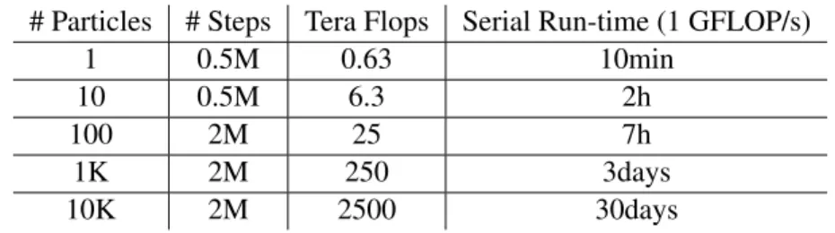
Plasma physics applications are math intensive applications. In table 1.1 we have the time consump-tion of the SOLCTRA, a software to simulate plasma physics, for a small number of particles and an estimation of the time for a high number of steps and particles.

# Particles # Steps Tera Flops Serial Run-time (1 GFLOP/s)

1 0.5M 0.63 10min

10 0.5M 6.3 2h

100 2M 25 7h

1K 2M 250 3days

10K 2M 2500 30days

Table 1.1: Approximation of the execution for the serial SOLCTRA application.

In the table, we can see that for the cases when a scientist wants to simulate a high number of particles and/or a high number of steps (this will help him to achieve more accurate results) he might have to wait up to a month. And we all know that a model like that is not sustainable. For a case like that, the results might be late and for the scientist it would be faster to develop a real life experiment, even when it is more expensive or dangerous.

The challenge we face is: can we improve a plasma physics simulation application by exploding these parallel architectures? And if so, what level of parallelism can it be achieved and how much would it be the maximum improvement?

1.3 Hypothesis

On this dissertation we propose that by having the right configuration and setup, an application for plasma physics simulation can be parallelized to achieve an efficiency of 0.8 on massively parallel architectures.

1.4 Objectives

1.4.1 Overall Objective

(15)

1.4.2 Specific Objectives

• Identify parallelization opportunities in plasma physics simulations.

• Evaluate architectural features in massively parallel processors Intel Xeon Phi to optimize plasma physics simulations.

• Explore mechanisms to match algorithmic and architectural features to accelerate plasma physics simulations.

• Evaluate and quantify the scalability of a parallel application on plasma physics.

1.5 The Approach

The overall objective of this thesis is to evaluate and understand the architectural features of massively parallel processors to accelerate plasma physics applications. This, by implementing vectorization and distributed and shared memory, while maximizing the speedup and the efficiency of the application.

To prove that a plasma physics application can be accelerated by implementing parallelism, we selected one application, the SOLCTRA, and within the application added vectorization and shared memory and distributed memory in a hybrid memory model.

• Vectorization: Vectorization is one implementation of the SIMD technique (Single Instruc-tion, Multiple Data). This is a feature that most of new processors include at some level. We can find that some processors have more power on vectorization than others. Following in this text, we will go deep into what vectorization is and how we implemented into the selected plasma physics application.

• Shared Memory: Shared memory is a paradigm based where a single process spawns independent threads which share the same address space. This is intended for small tasks where the threads could be created and destroyed several times across the application execution. This is also usefull when the different cores are sharing the same memory RAM.

(16)

• Hybrid Model: The hybrid models is when we mix the shared and the distributed memory paradigms. This is intended for cluster architectures where the application is being executed across several nodes, each of theses with more than one core.

1.6 Contributions

The major contributions of this thesis are:

• Understanding of a plasma physics code and opportunities for speeding it up with parallel computing. Part of the work of this research was to understand and study a plasma physic application to seek performances improvements through parallelism techniques, such as vectorization, shared, and distributed memory models.

• An experimental evaluation of a plasma physics code on top-of-the-line massively parallel architectures, exploring the features offered by the architecture and exposing the strengths and weaknesses of this architecture on a CPU-bound application such as the plasma physics application. We performed and evaluation and quantification of the scalability of a plasma physics application on multiple HPC architectures.

• A performance improved plasma physics simulation application for the local plasma com-munity. The plasma physics application that we used for our research is an application of the Plasma Physics Group at the Costa Rica Institute of Technology. During the work of this research we improved the application, moving from taking hours and even days for one execution, to take just a few minutes.

1.7 Thesis Overview

The rest of this thesis is organized in chapters covering the most important knowledge areas relevant to the discussion. Beginning from the general concepts to particular results for every proposed experiment.

(17)

Then, chapter 3 is intended to show the work on implement parallelism on a plasma physics application and the results of this implementation on a multicore architecture as is the Stampede supercomputer.

Once shown the results of the application on a multicore arhitecture, in chapter 4 we show the experiments results of the same application, but on a manycore architecture as it is the latest Intel Xeon Phi,Knights Landing(KNL), processor.

(18)

Chapter

2

Background

2.1 Massively Parallel Architectures

2.1.1 Multicore

Around the year 2005 [23], the processors started to hit the "heat barrier". That means that there is a point where instead of increasing the frequency of the processor, the power is consumed by heat and cooling the processor becomes one of the main efforts and commercial concerns. On the other hand, the need to increase the processing power is driven mainly by architectural advances. This power-performancedilemma pushed vendors to focus onmulticoredesigns. [12]

A multicore processor is a processor with multiplesubprocessorsorcores, where each one of these is capable of fully support at least one hardware thread [23]. The technical motivation behind this is the observation that the power dissipation of the CPUs is around the third power of clock frequency. So, by reducing the clock frequency, the vendors are able to place more than one core into the same die/package while keeping the same power envelope. [12]

When there is more than one core inside a die or package, there are some considerations to keep in mind:

(19)

• Integrated memory controller: previously, the memory controller was out of the die. Now, with multicore designs, it was moved inside the die. This helped on reducing the latency on accessing main memory and increased the velocity of intersocket networks.

We can find this kind of processors in most of today computers, from a smartphone like the Google Nexus 6, which has 4 cores, to the latest Intel Xeon processor, which has 24 cores.

2.1.2 Simultaneous Multi-Threading and Hyper-threading

Simultaneous Multi-Threading (SMT) is a technique to improve performance on the processor. Instead on focusing on higher clock speeds which increase the size of the die and the power consumption, SMT seeks improve the performance by having multiple threads executing on one processor without context switching. Unlike other techniques, SMT maximize performance without adding significant power consumption [29] and only requires some extra hardware instead the multicore [2].

Hyper-threading is the implementation of SMT on Intel’s architecture. It makes one single core appears as two logical cores to the operative system by replicating the architectural state of each thread or logical core, while sharing the physical execution resources among them [2, 26]. This increase the processor utilization and reduce the performance impact of I/O latency by overlapping the latency of one thread with the execution of the another. For the sharing resources, we can find three policies for sharing resources: partition (equal resource per thread), threshold (limited flexible sharing) and full sharing (flexible sharing without limits). [29]

The side effects of this implementation are not well-know and they will depend on each application. This is because simultaneous sharing of resources might create a potential performance degradation of the hardware.[2, 21]

2.1.3 Manycore

The next step for multicore platform is the manycore platforms. We can describe a manycore processor as a processor with so many cores that in practice we do not enumerate them; there are just “lots” of cores. This term is generally used for processors with 32 or more cores, but there is not a precise definition or an exact bound for a processor to be called from multicore to manycore processor. [23]

(20)

say that currently there are two main approaches: GPUs and the Intel Xeon Phi processor/coprocessor. Now we are going to describe each of these.

2.1.3.1 Graphic Processor Unit (GPU)

While a regular processor consists of a few cores optimized for sequential serial processing, a GPU has a massively parallel architecture consisting of thousands of smaller, more efficient cores designed for handling multiple tasks simultaneously [24]. As its name stands for, the GPUs were originally designed for graphics processing, but they have become general-purpose enough to be used for other purposes, taking advantage of its parallelism. [23]

For programming purposes, the GPUs can be programmed using a API called OpenCL or, in case of NVIDIA, a proprietary language called CUDA [23]. The focus on programming GPUs is to have most of the application code executed in the main CPU, while having the compute intensive parallelizable application code executed on the GPU. [24].

2.1.3.2 Coprocessor

Similar to a GPU, acoprocessoris an external card connected, mostly, through the PCIe port that can be used for additional computational power. The application that uses acoprocessorcan work as a native application on thecoprocessor, where basically the application is executed completely on thecoprocessor. Alternatively, using anoffload approach, similar to the GPUs, most of the application is executed on the host and the compute intensive is offloaded and executed on the coprocessor.

Nowadays, the main coprocessor in the market is the Intel Xeon Phi. The first generation of the Intel Xeon Phi was acoprocessorwith from 57 to 61 cores. This was in essence a manycore processor trapped in a coprocessor body.

But, thecoprocessorhas its limitations. Since acoprocessoris a PCIe device, it is limited to the memory inside its package and does not have direct access to the main memory of the machine. Also, since thecoprocessoris fed by the host processor, the data transfer will be back and forth between them, making the data bandwidth a potential issue on performance. These limitations pushed the programmers to look forward for an Intel Xeon Phiprocessor. [16]

(21)

programming in the same way as we could for an Intel Xeon processor system, but with extra attention on exploiting the high degree of scaling possible in the Knights Landing.

The major difference between the GPUs and the Intel Xeon Phi is that while a GPU accelerate some applications through scaling combined with vectorization, they do not offer the programmabil-ity of a Knights Landing. Applications that show positive results with GPUs should always benefit from Knights Landing because the same fundamentals of vectorization or bandwidth are present in that architecture. The opposite is not true. The flexibility offered by the Knights Landing includes support for applications that cannot be executed on a GPU. For example, while Knights Landing supports all the features of C, C++, Fortran, OpenMP, etc, GPUs are restricted to special GPU specific models, like NVIDIA CUDA, or subsets of standards like OpenMP. Therefore, the Knights Landing offers broader applicability and greater portability and performance portability. Also, tuning and debugging an application on a GPU is rather difficult in comparison with an architecture like the Knights Landing.

2.1.4 Clusters

When we talk aboutmulticoreandmanycorewe are talking about cores inside the same die/package. But, what about having cores not in the same die or even in the same computer. That is a cluster. A cluster is a distributed memory system composed by a collection of systems connected by an high-speed interconnection network. On a cluster we have n nodes interconnected where each of these nodes can be any kind of processing machine, from single-core nodes to manycore machines. Nowadays, it is usual to find clusters whose nodes are multicores or manycores with shared-memory.[25]

2.2 Performance Metrics

When a programmer is working on parallel computing, it is because that programmer wants to increment the performance of his application. That is the main objective of parallel programing. But, what is performance? As we can find in [23], performance can be seen as:

• The reduction of the total time for a computation.

(22)

Performance can be measured empirically on real hardware or estimated by using analytic models based on ideal theoretical machines. Empirical measures account for real world effects, but often give little insight into root causes and therefore offer little guidance as to how the performance can be improved or what could it be limited by. On the other hand, analytic measures ignore some real world effects but give insight into the fundamental scaling limitations of parallel algorithm. These approaches also allow the programmers to compare parallelization strategies at a lower cost than going directly into the implementation.

2.2.1 Latency and Throughput

Now, we are going to present some concepts related to performance theory, starting with the basic ones, such as latency and throughput.Latencyis the time it takes to complete a task and for this document we denote it asT. Throughputis the rate at which a series of tasks can be completed. While latency is measured in unit of time like seconds (s), the throughput is measured in works per unit time, and while a lower latency is better, a higher throughput is better. [23]

2.2.2 Speedup and Efficiency

Having defined the latency and throughput, we can define the speedup and efficiency.Speedupis the ratio of the comparison between the latency of an identical computational problem on one hardware unit or worker (also called the serial latency, depending on the consulted literature like [25]) versus that work onP hardware units (or the parallel latency). The speedup equation is defined in 2.1 [23].

Speedup=SP =

T1

TP

(2.1)

whereT1the latency taken by the computational work with a single worker, whileTP is the latency

taken by the same work onP workers. [23]

Efficiencymeasures the return of investment (ROI), and is defined by the speedup between the number of workers:

IfT1is the latency of the parallel program running with a single worker, the equation in 2.2 is

(23)

original serial algorithm, 2.2 is calledabsolute speedup, because both algorithms are solving the same computational problem.

Something that we as scientists have to be aware of and careful about is that using an unneces-sarily poorT1as baseline could inflate the speedup and efficiency. Also, we always have to be clear

and show both, speedup and efficiency, because while speedup can be a large number, the efficiency is a number between 0 and 1. A speedup of 100 sounds better than an efficiency of 0.1 even when we are talking about the same program/hardware [23].

Ideally, the efficiency would be 1, this is called aslinear speedup, but it is unusual to achieve. Also, it is expected that asP increases theE will become smaller [25]. However, we could find some exceptions of applications with efficiency higher than 1. Cases like this are calledsuperlinear speedup. We can find causes of this kind of behavior in cases like:

• If we use absolute speedup on cases when we are using different algorithms on the serial and the parallel applications. We have to be careful with this.

• Sometimes, the restructuring made for the parallel executions could improve the cache usage and handling.

• The performance of an application is being limited by the cache accessible for a single worker, so, adding more workers would increase the cache size accessible for the program, allowing the program to improve its performance.

• Parallelizing an applications could allow it to avoid extra work that its serialization could force.

2.2.3 Amdahl’s Law and Gustafson’s Law

What does make an application to not achieve a linear speedup? In the 60s, Gene Amdahl made the observation that unless virtually all of a serial program is parallelized, the possible speedup is going to be limited, no matter the number of workers available [25]. This is known as theAmdahl’s Law. This argued that the latency of a program falls into time spent doing non-parallelizable work (Wser)

and parallelizable work (Wpar). So, givenP workers we can say that:

T1 =Wser +Wpar ; TP ≥Wser+

Wpar

P (2.3)

(24)

SP ≤

Wser+Wpar

Wser +Wpar/P

(2.4)

Now, let say thatf is the non-parallelizable fraction of theT1. By substitution we can get the

speedup in terms off:

SP ≤

1

f+ (1−f)/P (2.5)

So, the maximum speedup achievable whenPtends to infinite will be:

S∞≤ lim

And with this, the conclusion of Amdahl’s Law is that the speedup will be always limited by the fraction of work that cannot be parallelized.[23]

A consideration with Amdahl’s Law is that it does not take into consideration the problem size [25]. Jonh Gustafson noted that the problem size grows as computers become more powerful and as the problem size grows the parallel part grows much faster than the serial part. This is known as Gustafson’s Law. So, from the equation 2.6, iff decreases, the speedup will be improved. [23]

In the end, both approaches are right. It will depend on the given problem if it is about running the same problem faster or running at the same time a bigger problem.

2.2.4 Scalability

Scalabilitycan be defined as the ratio on where a technology can handle ever-increasing problem sizes. Applied to parallel computing, if we can increase the problem size at the same rate of the number of workers that the efficiency remains the same, then we can say that the program is scalable. [25]

Matching the Amdahl’s Law and Gustafson’s Law from section 2.2.3 to scalability we can find two special cases: [23, 25]

• Strong scalability: This is the case for Amdahl’s Law. If the number of workers is increased and the efficiency is unchanged without increase the problem size, the application is said to bestrongly scalable.

(25)

2.3 Parallel Programming

On section 2.1.3 we mentioned two paradigms: shared memory and distributed memory. Based on how the hardware setup, the programmer can take one of those two approaches on parallel programming or an hybrid of both if the hardware allows it. On shared memory we can find several APIs or languages such as OpenCL, OpenMP and CUDA (for GPUs). While there can be found several choices on shared memory, on distributed memory there is one mostly used API: MPI (Message Passing Interface). Something to keep in mind is that the paradigm of shared or distributed memory is something at higher level of abstraction of the hardware. Therefore, besides one paradigm can be limited or improved by one of the types of hardware architectures seen in 2.1, they are not strictly attached to a hardware architecture in specific.

Additionally, if we have shared or distributed memory, the programmer has to be also worried about vectorization, which is a SIMD (Single Instruction Multiple Data) process where the compiler takes into account the processor capabilities and compiles certain groups of operations into vector instructions. [25]

2.3.1 Vectorization

We are starting with vectorization because it’s the first step on parallelizing an application, since taking this into the application could decrease the size of the problem by using the very same hardware and the workload for each future worker.

SIMD systems are parallel systems that operate on multiple data streams by applying the same instruction to multiple data items. This could be a system with a single control unit but multiple ALUs (Arithmetic-Logic Unit) or vector processors. Vectorization applies to vector processors. [25] A vector processor or VPU (Vector Processing Unit) is a processor capable to operate on vectors of data instead of a conventional CPU that can operate only on scalar data. To perform this, a VPU must have among other features vector registers and vector instructions to apply to those vector registers. So, in vectorization the compiler will generate assembly code to those vector instructions and registers, instead of creating assembly code to use the regular ALU [25]. For example, the Knights Landing processor supports vector register/instructions of 512 bits, allowing it to handle 16 single precision or 8 double precision mathematical operations at the same time, instead having to perform 16 or 8 separated instructions [16].

(26)

that can be vectorized. The second relies on the programmer, and it is basically to vectorize the application by explicit usage of libraries or SIMD languages directives.

In [16] we can find a methodology to achieve vectorization that we summarize next: 1. Measure baseline release build performance.

2. Determine hotspots.

3. Determine loop candidates by using compiler reports.

4. Use a vectorization analysis tool to identify the components that will benefit most from vectorization.

5. Implement vectorization recommendations.

6. Repeat the process until performance is achieved or there is vectorization left identified. Something really important to achieve high performance on vectorization is the data layout. This is important since a bad memory layout would push the compiler for a non-optimal vectorization, requiring some extra instructions and data access that will reduce the performance. To improve the memory layout, memory alignment is required.Memory alignmentis a method to force the compiler to create data objects in memory on specific byte boundaries. This is done to increase the efficiency of data operations to and from the processor.

The memory alignment leaves the programmer with two tasks: align the data and make sure that the compiler knows that the data is aligned through language directives.

2.3.2 Shared Memory with OpenMP

Ashared-memoryapplication is an application that is parallelized at the thread level. In here, the different workers share the physical address space [12]. On this paradigm the variables can be shared or private. Therefore, when developing a shared memory application, the programmer must be careful on the memory access of the shared variables and use synchronization to access them if it is required. Avoiding synchronization could create race conditions and lead applications to have non-deterministic behavior and wrong results. [25]

(27)

All the different OpenMP directives have their own options or configurations that the programmer must test and play with in order to find the configuration that fits better in the hardware/problem combination. For example, depending on if we are decomposing the problem from a task perspective or a data perspective [22], we could configure the OpenMP directive to set the affinity and distribute the threads scattered or compact through the different processors.

In any OpenMP application, a single thread runs from the start. Then, the user defines parallel regions where the master thread forks and joins a team of threads that executes the instructions inside the region concurrently.

(28)

value prompted to be saved in the variable.

2.3.3 Distributed Memory with MPI

Starting from what we saw on the previous section, we can say that differently to shared-memory, a

distributed memoryis an application that is parallelized at the process level. Hence, the address space is exclusive. This non-shared memory model breaks the restriction of having the different processes being executed on the same physical machine, allowing to have node-level parallelism in a cluster (see section 2.1.4).

Since the memory is distributed, the programmers need to explicitly transfer data between the different processes and nodes. This can be achieved by message passing through the OS. Today, this message passing is implemented in most of distributed memory application by using the MPI API.

MPI(Message Passing Interface) is a library that defines a set of more than 500 functions s [12] called from C/C++ or Fortran. In an MPI application, multiple instances orranksof the same program run concurrently and use the library routines to communicate between each other by exchanging messages. From the perspective of the programmer, the place where the ranks are being executed and how the communication is between them could vary without affecting the behavior of the application. [16]

Between the set of functions that MPI includes, there are functions for operations such as send, receive, and broadcast, and more advanced operations like gather, scatter, and reduction. MPI also provides operations for process synchronization, such as barriers, and also provides options for message passing synchronous or asynchronous. An additional requirement that MPI has, is that an MPI program cannot be executed on its own, it needs of a set of wrappers for its execution. [25]

In figure 2.2 we have a code that solves the same of the code of figure 2.1, but implemented using MPI. We have to clarify that these two examples are examples and might not be fully functional. In every MPI code, we have an opening and a closure calls, which are theMPI_Initand the MPI_Finalize. Outer those functions there is no MPI functionality available. In this example, first we request for communicator size and therankof the current process. These values work as the total count of process being executed and theidto the calling process.

(29)

int main(int argc, char_{** argv)}

MPI_Reduce(&myError, &error, 1, MPI_DOUBLE, MPI_MAX, 0, MPI_COMM_WORLD; MPI_Finalize();

}

Figure 2.2: C++ example with MPI

2.4 Plasma Physics Applications

Nowadays, in the plasma physics community, there is not a standard software for simulations, instead there are several simulation applications developed based on the specific requirements of the given group. We researched on the state of the art on the main applications currently used by the plasma physics community for plasma physics simulations.

(30)

2.4.1 Epoch

EPOCH is the Extendable PIC (Particle in Cell) Open Collaboration project developed for the CCP-Plasma (Collaborative Computational Project in Plasma Physics) UK community [14]. It is a plasma physics simulation code which uses the PIC method where collections of physical particles are represented using a smaller number of pseudoparticles. It calculates the fields generated by the motion of these pseudoparticles, then uses the force generated by those fields to calculate the velocity and then the velocity to update the positions of the pseudoparticles. At the end, this works to reproduce the behavior of a collection of charged particles. [3]

Currently, this application has been parallelized by using MPI and used dynamic load balancing for optimal usage of the processors.

2.4.2 BOUT++

Also under the CCP-Plasma, BOUT++ is modular C++ 3D plasma fluid simulation code developed at York in collaboration with the MFE group at LLNL and the MCS division at ANL [14]. It has been developed from theBoundary Turbulence 3D 2-fluid tokamak edgesimulation code BOUT. Among the features that BOUT++ has we can cite: arbitrary number of scalar and vector fluid equations solver, time integration schemes and it has implemented high-order differencing schemes, generalised differential operators. [11, 10]

On parallelization, BOUT++ can be parallelized on two dimensions. It has enabled the usage of PETSc, which is a library for partial differential equations. This library supports MPI and GPU parallelization through CUDA and OpenCL.

2.4.3 NESCOIL

NESCOIL (NEumann Solver for fields produced by externals COILs) is a code for the calculation of the surface current on the exterior surface of two toroidally closed surfaces such that the normal field on the interior surface is minimized [18]. This code has been an important coil design tool for large aspect ratio stellarators.

In terms of parallelization, currently there is no public information on the state of this application.

2.4.4 VMEC

(31)

energy of the system [19].

2.4.5 SOLCTRA

SOLCTRA is a CPU-bounded code used on development of the SCR-1 (Stellarator of Costa Rica 1) by the Plasma Group of the ITCR (Costa Rica’s Institute of Technology). [31]

The SOLCTRA code was used to calculate the magnetic fields and the magnetic structure that confines the plasma produced by the twelve modular cooper coils on the SCR-1. These magnetic fields are important to define the best electron cyclotron frequency heating (ECH) system. These magnetic fields are also needed to evaluate the confinement of the device. [30]

This application was initially written in Matlab in order to draw the generated magnetic fields by the coils on a complex way. To solve this, the application uses a Biot-Savart solver and a reduced model of the twelve modular coils of the SCR-1. The application estimates the 3D magnetic field, magnetic surfaces, rotational transform profile and magnetic well. [30]

During the SCR-1 development, performance issues were found on the Matlab code related to the estimation of the magnetic fields. That pushed the team on migrate that section of the code to C++, splitting the application in two parts: the computationally intensive one in C++ for the magnetic fields simulation and calculations and the light one in Matlab for the drawing of the magnetic fields resulted on the module in C++.

To calculate the magnetic fields, the application implemented a fourth order Runge-Kutta’s method based on [5] and [17].

At high level, the code first load the information of the twelve modular coils, one Cartesian point per grade. This information needed to be loaded only once per iteration and remains constant thought all program execution.

After the load of the coil information, the tool has to calculateeˆn, which is defined as the unit

vector along each segment of each coil [13]. This value is calculated as the difference between the next point and the current point divided by the norm of the current point (see Fig 2.3).

ˆ

en= Pn+1_norm−₍_PnPn₎

Figure 2.3: Formula to calculate the roof of the n point

Once we have the coil information loaded and theeˆnfor every point, a loop is executed to get

(32)

Note that the roof calculation has to be made only once for all the execution. This is because the coils are fixed, hence theˆenare same for all the Runge-Kutta calculations.

P0←StartP oint

loop

K1←MAGNETIC FIELD(P0)

P1 ← K1₂ +P0

P2 ← K2₂ +P0

P3 ←K3+P0

P0 ←P0+K1+2∗K2+2₆ ∗K3+K4

end loop

Figure 2.4: Pseudo-algorithm for the fourth order Runge-Kutta

(33)

Chapter

3

Parallelizing a Plasma Physics

Application: SOLCTRA

For the purpose of this research, we worked on the SOLCTRA application (see ssection 2.4.5). In this chapter, we will present the work on the parallelization of the SOLCTRA application and how we implemented vectorization, distributed memory and multithreading to improve the performance of the application. Additionally, we will present the Stampede supercomputer of the Texas Advance Computer Center and the results of the execution of the paralyzed SOLCTRA, in the Stampede platform.

3.1 Code Cleaning

The original code was written in Matlab and then migrated to C++, but, this migration was not made keeping performance or C++ code practices in mind. It was just a code translation from Matlab to “C++”, which was more a translation to an old C. Because of that, before implementing any parallelization technique, we had to clean up the code so vectorization, distributed memory and multithreading implementation could be easier.

Besides making the code more readable and understandable, another major reason that pushed us to start with cleaning the code is that, as we can find in [32], some simple changes can help the compiler to improve the efficiency of the generated binaries.

(34)

code from doing that, to do onefopenbefore the start the algorithm execution for every given point and afcloseat the end, allowing during the iterations to only have one I/O operation, the writing of the result of the iteration.

AnotherBest Known Method(BKM) from [32] is to change several divisions with the same divisor (see 3.1a) into the multiplication of the inverted of that divisor (see 3.1b). This is based on the fact that a multiplication takes fewer CPU cycles than a division.1

double result, divisor;

Figure 3.1: Division transformation into the multiplication of the inverted divisor.

Also, in the application we have several structures that were at global level. This is a bad software development practice, so we changed the application to make those structures local and pass them as parameters to whoever needs them.

The previous changes were made by just reviewing the code. But to get a better picture of the performance issues of the applications we had to start using the Intel VTune Amplifier. This tool is a performance profiler that assists the developer on finding issues and the bottlenecks of the code. The first time that we executed the analysis tool we got the results from figure 3.2 where the operationspowandsqrtwere the ones that were taking most of the execution time. From a parallel computing perspective, these functions can be marked as noise because we cannot make

1

(35)

them parallel themselves, but it does not mean that they cannot be improved. On the case of thepow operation, the exponent was always2, so we changed the operationpow(a,2)for a multiplication: a*a. For thesqrtoperation, there was no way to improve it and that was something that had to stay in the code.

Figure 3.2: Analysis results on the original code version of SOLCTRA

After implement the changes above, we decided to start on the parallelization work as is shown on the next section.

3.2 Implementing Distributed Memory, Vectorization and

Multithreading

In section 2.3 we introduced the concepts of MPI, Vectorization and OpenMP. In this section we are going to talk more deeply about these frameworks and show how we had applied them into the SOLCTRA application.

3.2.1 Implementing Distributed Memory

For the distributed memory we used MPI. On this implementation we have to split the application into two parts. The first one is going to parse the parameters, load the coil information and calculate theeˆn (see section 2.4.5). The second one is the one that iterates on the list of start points per

particle and executes the Runge-Kutta algorithm for each of those start points.

(36)

For the second section of the code, after reviewing the code, we noted that the algorithm executions for every particle are completely independent on each other. This led us to implement the MPI parallelization at the particle level. With this, when the application receives a list of start points, for each particle, the application is going to distribute them among the MPI ranks that the application has (see figure3.3). One of the reasons of implementing the MPI parallelization is that there is no need of adding any MPI communication between the ranks for this section of the code, which could lead to overhead during the execution of the application.

Figure 3.3: MPI implementation with particles independently distributed across MPI ranks.

3.2.2 Implementing Vectorization

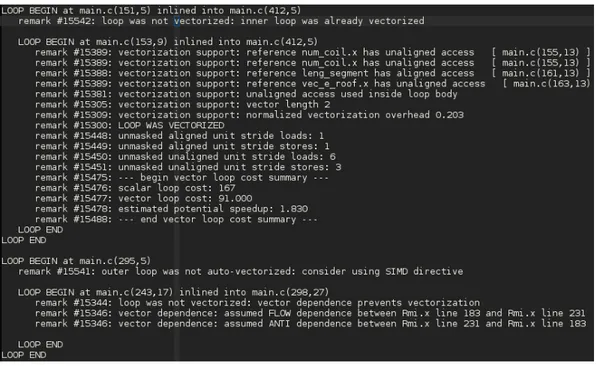
To start on the vectorization we took the compiler report2and the Intel Advisor. Those tools helped us on finding issues and vectorization opportunities.

In figure 3.4 we can see that how the compiler is reporting issues on vectorization due to unaligned accesswhich can decrease the vectorization performance or block it completely.

Meanwhile, on figure 3.5 we can find that we have a vectorization opportunity on themagnetic_field function that has not been vectorized due dependencies assumed by the compiler.

Unaligned data is one of the major constraints for vectorization, so, we changed the code to use aligned data. Above, we described the data structures that were global and we moved them to a local scope. These structures were not aligned since they were AoS (Array of Structs, see figure 3.6a).

2

(37)

Figure 3.4: Example of the compiler report on vectorization

Figure 3.5: Vectorization analysis results on the original code version of SOLCTRA

Because of that, the first improvement that we did was to attack them in order to transform them into SoA (Struct of Arrays, see figure 3.6b).

With the SoA implementation, we also have to change the way code handles the memory. Originally, the memory was allocated statically in the stack. By using this way, the developer does not have the control to allocate the memory in an aligned way. Additionally, we had not used the mallocfunction for the memory allocation since this does not have the capability to force the memory alignment required for vectorization. Instead, we used the_mm_malloc, which receives an additional parameter to force the alignment (see figure 3.7).

(38)

struct cartesian

Figure 3.7: Implementation of the_mm_mallocfunction for memory allocation.

followed the code execution. Therefore, the first loop that we attacked, was on the function to get the length of each segment and theˆe, at the beginning of the program, and the calculation of the vectors from each segment end points to the observation point [13]. Once having the AoS to SoA code implementation and the use of the_mm_mallocfunction, the vectorization of theeˆwas as simple as mark the for loop with thepragma ivdepmacro (see figure 3.8). When we were sure that the memory was aligned, we also added apragma vector alignedmacro to explicity indicate to the compiler that the memory of the array is aligned. We have to clarify that sometimes the compiler could determinate that the loop can be vectorized, but we have to add those macros to explicitly mark the given for loop and help the compiler on this task. We continued doing similar until all the innermost for loops were vectorized.

3.2.3 Implementing Multithreading

(39)

#pragma ivdep

Figure 3.8: Vectorization of one loop in SOLCTRA.

3.2.3.1 Adding threading

The places selected to add threading with OpenMP was on themagnetic_fieldsand another function called insidemagnetic_fields. These two functions had a common structure with two nested loops, where the outer loop iterates per coil and the inner one on the coil information.

During this process we noted that the size of the problem per particle is defined by the quantity of coils and the information of each coil. So, it is fixed to12∗360iterations. With that, on this stage we parallelized these sets of for loops at the outer level, allowing a maximum threading of 12 per particle. At this point, it was as easy as just add theomp parallel forpragma above each outermost for loop inside those functions as is shown in figure 3.9.

#pragma omp parallel for

for (int i = 0; i < TOTAL_OF_COILS; i++) {

// Do something

}

Figure 3.9: Adding threading through OpenMP to SOLCTRA.

(40)

into another. To solve this predicament, we implemented a solution showed in [32]. This solution consisted on creating a temporary array where each thread will save the results of its calculations and, when the parallel region is done, the main thread iterating on these arrays. A collateral change, we had to split theomp parallel forfor that loop so we could initialized the variables per thread (see figure 3.10).

(41)

3.2.3.2 Moving from pragmaivdepto pragmasimd

Other change that we did was to change thepragma ivdepmacro for the OpenMPpragma omp simdmacro for two reasons: a) thepragma ivdepis not an standard and only applies for some compilers, and b) that according to [12] and [16], while the pragma ivdepis an explicit hint to the compiler, thepragma omp simdmacro forces the vectorization. This is not without a risk. Since with this mode the compiler does not perform any check on alignment or possible data issues, the responsibility relies on the developer. With this change, we also have to add areductionclause to thepragma omp simdper variable that was accumulating the calculations.

At this point, we started to execute the application with the Intel VTune Amplifier again after the first stage of parallelization. With this we found that every time that themagnetic_fields function is called, it was allocating memory for the temporal variables and it was taking sig-nificant time. Since the data was always written first on the function called at the beggining ofmagnetic_fieldsand then read for the rest of themagnetic_fields function, there was no chance to read dirty values. Because of those reasons, we move the memory allocation to an upper level of the application call stack and adding those vectors as parameters of the magnetic_fields. With this change we moved the application from performing four memory allocations per iteration to perform only one memory allocation per Runge-Kutta execution.

Even with the previous change, the performance related to this temporary calculation was low. Because of that, we focused our efforts on how to get rid of these vectors and the function called bymagnetic_fields. But those temporal arrays were used only on the loops inside the magnetic_fieldsand there was not a cross index calculation (the i-th value was used only by the i-th iteration). Therefore, there was no need to calculate those values before they were going to be used. This change allowed the application to get rid of an unnecessary for loop affected by load imbalance without changing the results of the application, improving the performance of the application by around 9%.

3.2.3.3 Strip-Mining Implementation

(42)

workers will have work to do and the other 4 will have to wait those to finish. On the other hand, if we have 16 workers, what we are going to have is that 12 workers are going to be busy but 4 are going to be unused at all, which is a waste of resources.

To solve this predicament, we implemented a technique calledstrip-mining. This technique consist in transform a for loop into two nested for loops by splitting the data intostripsortiles, so the outer loop iterates on the per strip and the inner iterates inside the strip [32]. In figure 3.11 we have an example of how the original for loop 3.11a is transformed into two 3.11b.

for(int i=0; i<n; ++i)

In[32], the authors recommend to select the size of the tiles to be a multiple of the vector length so the strip-mining implementation will not interfere with the vectorization in the inner loop. To avoid false sharing across the different cores, we decided to not use the vector length. Instead, we decided to use the page size so every thread will be accessing its own independent page on every iteration. In our application we are working with thedoubledata type, which has a size of 8 bytes, and since the page size is of 64 bytes so we are able to fit 8 values in the inner loop.

(43)

for (int jj = 0; jj < TOTAL_OF_GRADES; jj += GRADES_PER_PAGE)

Figure 3.12: Strip-mining implementation in the SOLCTRA application.

WhereTOTAL_OF_GRADESis the total of grades per coil (360) andGRADES_PER_PAGEis the quantity of grades that fits into one single page (8). So, since the last iteration will not fully fit into a single page, we have to add a check so the last iteration will stop at the end of the data and not at the end of the page.

Currently, we have shown how this implementation affected the inner loop of the two originals. Now we are going to explain what we have changed in the outer one and how it solved the predicament of maximum 12 threads.

#pragma omp for collapse(2)

for (int i = 0; i < TOTAL_OF_COILS; i++) {

for (int jj = 0; jj < TOTAL_OF_GRADES; jj += GRADES_PER_PAGE) {

(44)

In figure 3.13, we are showing how we have used thecollapse clause to increment the parallelism level of the application. This allows the application to add threading at a granularity level of the total of pages used, instead the total of coils. After this, we would be able to run, theorically, a total of540threads (see equation 3.14).

total=T OT AL_OF_COILS∗ _GRADEST OT AL_OF_{_}_{P ER}_GRADES_{_}_{P AGE}

Figure 3.14: Total of threads calculation after strip-mining and omp for collapse

3.3 Experiments on Stampede

Once we have modified the code, we started to run the application and collect data in a the Stampede supercomputer.

3.3.1 What is STAMPEDE?

Stampede is the main supercomputer of the Texas Advance Computer Center funded by the National Science Foundation of the USA. Deployed in 2012, the Stampede system is powered by Dell PowerEdge nodes with Intel Xeon E5 processors and Intel Xeon Phi (Knights Corner) coprocessors, the first generation of processors based on Intel’s (MIC) architecture. [28]

In this section we describe only the host architecture of the nodes. This is because at this stage of our research we were not focused on the Stampede’s coprocessors.

Each of the nodes consisted of two Intel Xeon E5-2680 of the Sandy Bridge family with 32GB of memory. These processors or sockets have a base frequency of 2.7GHz and each has 8 cores. Even though these processors includes the hyper-threading technology, the Stampede’s nodes have the feature off. An additional feature of these processors to our concern is that they include the AVX instruction set. This instruction set allows the user to use vector instruction of 256 bits wide, in our case to execute 4 operations at the same time with the proper vectorization.

In the experiments to follow, in order to have more reliable values, we executed least 10 times each configuration. So, the results that we are going to show are the average of those executions. The reason of using 10 is because our queue size on Stampede allowed us to run only 10 executions simultaneously.

(45)

• OMP_NUM_THREADS: This is a environment variable use to define and control the quantity of OpenMP threads executing everyparallelregion.

• Number of ranks: The number of ranks is set by the-nparameter of the MPI execution (mpirunormpiexec, andibrunin the cases of Stampede).

• Particles: The number of particles to simulate is set in the SOLCTRA application by the -particlesparameter. This is the only variable that we are going to set to modify the size

of the problem in all our experiments.

3.3.2 Weak Scaling Experiment Results

The first experiments we present are on the frame of the weak scaling. How we explained in section 2.2.4, the weak scaling is when the size of the workers increase as the same ratio as the size of the problem is increased.

For these experiments, we “played” with the different configurations of MPI and OpenMP, changing the quantity of ranks and threads to analyze the behavior of the application. We changed variables in exponents of 2. For the MPI we used the set of{1,2,4,8}and for OpenMP the set of

{2,4,8,16}. We did not analyzed the combination of MPI=1 and OpenMP=1 since it is the serial time. Instead, we used the average of that configuration as theT0. On the problem size, the number

of particles, for each experiment, we configured it equal to the MPI rank, so both are increased as the same ration while the particles per rank remain fixed.

In figure 3.15a we have the graph for the speed up achieved by the application on different MPI/OpenMP configurations. We can see that for all the OpenMP configurations the line is incremental as the MPI is incremented. Also, we can note on those lines that higher the OpenMP, higher the speedup, except for the OpenMP of 16. For that case, we can see that if follows a similar increment as the other lines but with a speedup lower than even the OpenMP of 2.

In figure 3.15b we have the results for the efficiency. In this figure we can see that overall the four lines follow the trend to be flat. The exception for that is for the lines of OpenMP set to 2, 4 and 8. In those cases we can see that there is an increment when the MPI pass from 1 to 2 for all the OpenMP. Also, similar to the speedup, we can see that there is a big difference between the OpenMP of 16 with the other configurations.

(46)

(a) Speedup. (b) Efficiency.

Figure 3.15: Experiment results of SOLCTRA on Stampede supercomputer for the weak scaling.

node. When we have a OpenMP thread count equal or lower than 8, all the threads remains in the same processor, but when the thread count is 16, the application has to use both processors for the same rank. This inter processor communication has a high impact on the performance. Other research [4] found there is a performance degradation when threads are spread across different sockets on the same node. Our experiments show the same phenomenon, which may be due to the cost of synchronization between threads on different processors.

From these experiments, we can say the the application is weakly scalable in the Stampede architecture while the threads remain in the same socket.

3.3.3 Strong Scaling Experiment Results

After the results of the weak scaling, we moved to run the experiments on the strong scaling. We saw in section 2.2.4 that strong scaling is when the size of the problem is fixed to a certain value while the number of workers is increased.

For these experiments on strong scaling we are going to use the OpenMP only on the values from 1 to 8. But again on the analysis we did not include OpenMP to 1 because that is theT0. We

(47)

all the configurations.

(a) Speedup. (b) Efficiency.

Figure 3.16: Experiment results of SOLCTRA on Stampede supercomputer for the strong scaling.

In figure 3.16a we have the speedup for the strong scaling results. In there we can see that the speedup increase at a ratio close to the number of MPI ranks for each OpenMP thread count. On the efficiency side (figure 3.16b), we can see an increment of the efficiency when the we pass from 1 to 2 MPI ranks, and then it remains almost unchanged for the other MPI ranks.

Since the efficiency is increased or flat when we increase the number of MPI ranks while having the size of the problem fixed, we conclude from these experiments that the application on this architecture is strongly scalable.

Additionally, we can note that the speedup and efficiency figures for weak scaling are quite similar to the figures for strong scaling with weak scaling lines a little bit higher than the strong scaling lines.

3.3.4 Incrementing the Size of the Problem While Keeping the Workers Fixed Experiment Results

(48)

For these experiments, we selected the configuration of 2 MPI ranks and 8 OpenMP threads per rank. We chose this configuration because the OpenMP=8 was the one that showed better balance between high speedup and high efficiency for both weak and strong scaling. In order to maximize the resources for execution and to fill up a whole node, we chose MPI=2. Then we executed the application with the particle’s count from2to32.

(a) Average speedup. (b) Average efficiency.

Figure 3.17: Results of SOLCTRA on Stampede supercomputer with fixed worker count.

On figure 3.17 we have the speedup (3.17a) and the efficiency (3.17b) results for this set of experiments. In there we can see that both remains linear from 2 particles to 32, from 1 to 16 per MPI rank. That was what we were expecting: to keep the speedup and the efficiency unaffected as the size of the problem got increased.

(49)

Chapter

4

Executing SOLCTRA on a Many

Integrated Core Architecture:

Knights Landing

On chapter 3 we showed the parallelization of SOLCTRA and the results of the application on the Stampede supercomputer. After having a successful test on a multicore system, the next step was to test the SOLCTRA application on a manycore system. For this experiments, we selected the second generation of the Intel’s Xeon Phi processor codenamedKnights Landing(KNL).

The main reasons of this selection was based on:

• Top of the line architecture: The Intel Xeon Phi Knights Landing is the latest processor in the many-core line. It was released in July of 2016. According to the latests top 500 list released in November, the top 5th supercomputer in world, Cori, was made using KNL [20].

(50)

4.1 Intel’s Xeon Phi Architectural Overview

In section 2.1.3 we introduced the concept of a many-core architecture and in section 2.1.3.2 specifically the Knights Landing. In this section we are going to do a deeper review of the architecture of the Knights Landing manycore processor.[16]

The Intel Xeon Phi Knights Landing is the latest processor of the the Intel’s Many Integrated Core (MIC) architecture family, which is the name used by Intel to identify its manycore processors and coprocessors. The previous product of this family was the Xeon Phi codenamedKnights Corner (KNC). In section 2.1.3.2 we introduced this coprocessor. In that section we also mentioned that it has several limitations like being constrained to the memory inside the package and the bandwidth of the PCIe connection with the host resources.[16, 8]

Differently to the Knights Corner, the Knights Landing is a standard standalone processor. Hence, it does not have the constraints related to memory and bandwidth of of being inside a PCIe package.[16]

Figure 4.1: Composition of Knights Landing’s tile.

(51)

Figure 4.2: Composition of Knights Landing’s mesh.

The Knights Landing processor has two types of memory, the MCDRAM for high bandwidth and the DDR for large capacity. The MCDRAM is integrated on the Knights Landing package with 16GB of capacity. These MCDRAM have their own memory controller called EDC. This can be configured at boot time to be used as cache of the DDR, to be an extension of the DDR (sharing the same address space), or a hybrid, where a percentage can be used as cache and the remaining as flat. The Knights Landing has two DDR4 memory controllers, allowing to handle until 384GB of DDR memory. [16, 9]

(52)

4.2 Enviromental Changes on Supercomputer

Opposed to Stampede which is a multicore architecture, with the Knights Landing we are moving from a configuration with 8 cores and threads per package, to a configuration of 64 cores and 256 threads per package. This change opens a spectrum of possible configurations, beyond the ones described in section 3.3.1 which might have an impact on the performance of our application.

Next, we are going to describe some additional settings that we changed to improve the perfor-mance of SOLCTRA on the Knights Landing.

4.2.1 Thread affinity

This is a configuration set through the environment variableKMP_AFFINITY. This variable sets how the OpenMP threads are distributed across the cores, and how they are distributed and bound inside each core. This is one of the more complex environment variables. This is because, differently to most of the variables related to OpenMP, the variable has several arguments toan be set. For our experiments we only care about thegranularityand thetype:

• Granularity: the granularity sets if each OpenMP thread (software thread) is bound to a thread of the core (hardware thread) or if it will be attached to the core but not to a specific thread inside that core. To have them attached to a thread inside the core, the variable has to be set tofine(orthread), and if we want them to move across the threads in the core, it has to set tocore.

• Type: the type sets how the threads are distributed across the different cores. For our experiment we only usedscatterandbalanced.

(a) Setting affinity type toscatter. (b) Setting affinity type tobalanced.

(53)

In figure 4.3 we have the distribution of four threads on a hypothetical hardware with two cores and four threads per core. For the scatteraffinity (4.3a), the threads are going to be distributed evenly across the cores as possible, following a round-robin distribution. Meanwhile, for thebalancedaffinity (4.3b), the threads are going to be balanced on the cores with continuous threads closed to each other, following a block distribution.

4.2.2 Loop scheduling

The loop scheduling defines how the different loops iterations are being scheduled across each OpenMP thread in a parallel forregion. It can be defined inside the code or through the environment variableOMP_SCHEDULE. It has two parameters, the schedule policy and the chunk size.

The chunk size is described as the number of loop iterations that each thread is going to execute on each of its iterations on the for loop. For example, if this value is set to 2 and we have 2 threads, when the thread 0 starts the loop, it is going to execute the first 2 iterations, then the thread 1 is going to execute next 2 loop iterations, then the thread 0 will execute the next 2 loop iterations, and so on (see figure 4.4).

Figure 4.4: Schedule example for two threads and a chunk size of two.

For our experiments we used the policies static, dynamic, and guided described as follow:

Parallelization of Plasma Physics Simulations on Massively Parallel Architectures