Design of a Logistics Nonlinear System for a Complex, Multiechelon, Supply Chain Network with Uncertain Demands

(1)

Research Article

Design of a Logistics Nonlinear System for a Complex,

Multiechelon, Supply Chain Network with Uncertain Demands

Aaron Guerrero Campanur,

1

Elias Olivares-Benitez ,

2

Pablo A. Miranda ,

3

Rodolfo Eleazar Perez-Loaiza,

4

and Jose Humberto Ablanedo-Rosas

5

1_{ITSUruapan, Tecnologico Nacional de Mexico, Carr. Uruapan-Carapan 5555, Uruapan, Michoacan 60015, Mexico} 2_{Facultad de Ingenieria, Universidad Panamericana, Prolongacion Calzada Circunvalacion Poniente 49,}

Zapopan, Jalisco 45010, Mexico

3_{Department of Engineering Sciences, Universidad Andres Bello, Quillota 980, Vi˜na del Mar, 2531015, Chile} 4_{ITApizaco, Tecnologico Nacional de Mexico, Av. Instituto Tecnol´ogico S/N, Apizaco, Tlaxcala 90300, Mexico}

5_{College of Business Administration, University of Texas at El Paso, 500 W. University Avenue, El Paso, TX 79968, USA}

Correspondence should be addressed to Elias Olivares-Benitez; [email protected]

Received 29 June 2018; Revised 3 October 2018; Accepted 28 October 2018; Published 12 November 2018

Academic Editor: Zhiwei Gao

Copyright © 2018 Aaron Guerrero Campanur et al. This is an open access article distributed under the Creative Commons Attribution License, which permits unrestricted use, distribution, and reproduction in any medium, provided the original work is properly cited.

Industrial systems, such as logistics and supply chain networks, are complex systems because they comprise a big number of interconnected actors and significant nonlinear and stochastic features. This paper analyzes a distribution network design problem for a four-echelon supply chain. The problem is represented as an inventory-location model with uncertain demand and a continuous review inventory policy. The decision variables include location at the intermediate levels and product flows between echelons. The related safety and cyclic inventory levels can be computed from these decision variables. The problem is formulated as a mixed integer nonlinear programming model to find the optimal design of the distribution network. A linearization of the nonlinear model based on a piecewise linear approximation is proposed. The objective function and nonlinear constraints are reformulated as linear formulations, transforming the original nonlinear problem into a mixed integer linear programming model. The proposed approach was tested in 50 instances to compare the nonlinear and linear formulations. The results prove that the proposed linearization outperforms the nonlinear formulation achieving convergence to a better local optimum with shorter computational time. This method provides flexibility to the decision-maker allowing the analysis of scenarios in a shorter time.

1. Introduction and Context of the Problem

Supply chain design is a critical strategy for achieving com-petitiveness in current global business environments. The supply chain consists of all functions involved, directly and indirectly, in meeting customer needs. Decision-making in supply chain management is classified into three hierarchical levels: strategic (long-term), tactical (medium-term), and operational (short-term). Frequently, these decisions are ana-lyzed and solved independently at each planning stage, which generates an overall suboptimal solution when compared to solutions from comprehensive models. Therefore, supply chain management demands the use of new strategies and technologies to meet the current challenges of economic

globalization [1], especially the highly dynamic behavior of customer demand. This characteristic imposes a greater chal-lenge in developing and designing responsive and efficient supply chain networks. The mathematical formulation in the operational planning stage is highly critical and must model the relevant characteristics of the supply chain.

Facility location problems, which are typically used to design distribution networks, involve determining the sites where to install resources, as well as the assignment of potential customers to those resources. This family of prob-lems typically assumes a linear cost function and a set of deterministic customer demand. These assumptions avoid modelling interactions between facility location and inven-tory management decisions. According to these facts, the Volume 2018, Article ID 4139601, 16 pages

(2)

(to be selected)

Retailers (to be selected)

Warehouses Plants

Suppliers

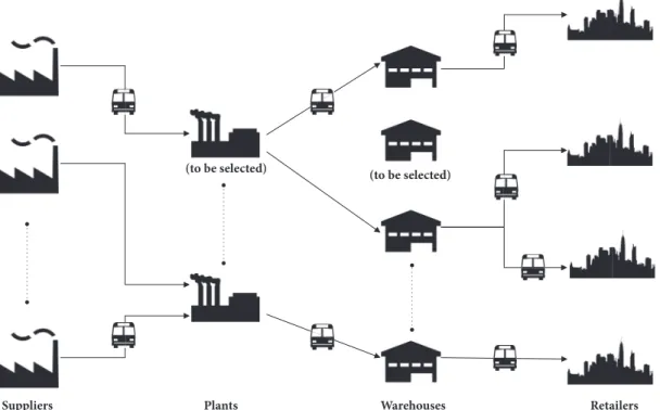
Figure 1: Four-echelon supply chain.

inventory-location research literature is aimed to integrate the demand uncertainty and the risk-pooling effect into supply chain network design [2].

This paper presents a mixed integer nonlinear pro-gramming formulation aimed to optimize the distribution network design. The model includes decisions on plants and warehouses location, transportation and assignment between facilities (plants-warehouses, warehouses-retailers), supplier selection, and implicit inventory decisions. The model is named a Four-Echelon Inventory-Location Prob-lem with Supplier Selection (4EILP-SS). The mathematical formulation models a four-echelon supply chain, with a set of potential sites for allocation of plants and warehouses, as shown in Figure 1. Each warehouse and plant has a limited capacity and manages a continuous review inventory policy to satisfy the demand of retailers and warehouses, respectively.

The objective is to determine the flow of material in each echelon and the location of plants and warehouses. Inventory management decisions are simultaneously modeled with the design of the distribution network. The problem of locating facilities is commonly used as a base for the design of supply chains. However, the effect of risk integration by inventory management decisions is not directly modeled by the classic facility location problem (FLP). Additionally, supplier selection is a relevant issue because it affects many important aspects of the supply chain performance. In some real cases, for example in the context of the automotive industry, it is common to consider the involvement of sup-pliers in the supply chain planning stage. Supplier selection is a complex process that involves identifying potential sup-pliers, requesting information, establishing contract terms,

negotiation, and evaluation. Several criteria are considered for supplier selection: quality, delivery time, price, service, and flexibility, among others. In the problem studied, we are assuming that the available suppliers were preselected considering several of the criteria described before, and the last decision was made based on the outcome of the opti-mization model that considers cost, lead time, and capacity. This is a common practice in industry, especially automotive industry, which is the motivation of this work, where an exclusive group of suppliers has the appropriate certifications by Original Equipment Manufacturers to participate in bids and requests.

Additionally, in the recent years, there has been an offshore moving of automotive manufacturing plants from industrialized countries to emerging economies. This hap-pened in China, India, Mexico, Brazil, Thailand, and Turkey, among others [3]. This required the design of new supply chains to meet the demand, including new plants and warehouses.

(3)

2. Literature Review

Inventory-location problems (ILPs) have been extensively studied over the past two decades. This section presents a review of the main contributions reported in the literature, showing trends in formulations and solution approaches. Although ILPs are extensions of Facility Location Problems (FLPs), this paper does not discuss the related FLP literature. Interested readers may consult Hamacher and Drezner [4], Daskin [5], Nickel and Puerto [6], Melo et al. [7], and Eiselt and Marianov [8, 9].

Jayaraman [10] studied a basic ILP, based on a mixed integer programming model for locating warehouses and sat-isfying customer’s demand for different products. The inven-tory modeling included the EOQ (Economic Order Quantity) model with fixed lot size and deterministic demand. Nozick and Turnquist [11] investigated an ILP, which included fixed warehouse location costs, and transportation and inventory costs. The problem was solved using a combination of a greedy and improvement algorithm. Erlebacher and Meller [12] presented an ILP with stochastic demands for a two-stage supply chain network, along with some heuristic procedures to solve a variety of instances. Another two-echelon ILP was studied by Nozick and Turnquist [13]. The model minimizes the inventory and unfulfilled demand costs. They used a combination of iterative greedy and improvement algorithms as a solution strategy. Nozick and Turnquist [14] analyzed a distribution system and the trade-off between facility costs, inventory costs, transportation costs, and customer responsiveness. They built an efficient frontier for assessing the different solution configurations.

Daskin et al. [15], Shen et al. [16], and Miranda and Garrido [17] presented similar versions of ILPs, proposing mixed nonlinear integer-programming formulations. The model considers a continuous control inventory policy with stochastic demand, the safety stock cost is determined by a chance-constrained approach, and the ordering decisions are based on the EOQ model with order quantities as decision variables. Daskin et al. [15] and Miranda and Garrido [17] solved the model using Lagrangian relaxation, while Shen et al. [16] reformulated the model as a set-covering problem, and developed a column-generation algorithm. Shu et al. [18] studied the column generation approach proposed by Shen et al. [16], showing that the pricing problem gives rise to a new class of the submodular function minimization problem. They discussed how the general pricing problem could be solved by exploiting certain special structures.

Snyder et al. [19] presented a stochastic programming-based ILP including some random parameters defined by discrete scenarios. The location model explicitly handles the economies of scale and risk-pooling effects that result from consolidating inventory sites. They used a Lagrangian relaxation-based algorithm. Shu et al. [20] proposed a two-stage stochastic model to address an integrated location, and two-echelon, inventory network design under uncertainty. They defined the problem as a two-stage nonlinear discrete optimization problem. The first stage decides which warehouses to open and the second one decides the warehouse-retailer assignments and the

two-echelon inventory replenishment. They used a set covering formulation transformed into a pricing problem, which was solved using column generation.

ILPs with inventory capacity constraints were analyzed by Miranda and Garrido [21, 22] and Ozsen et al. [23]. Ozsen et al. [23] introduced a 100% service level constraint for inventory capacity to a previous ILP presented by Daskin et al. [15], while Miranda and Garrido [21, 22] discussed how the inventory capacity constraint can be controlled by a previously defined service level (usually less than 100%), based on a chance-constrained formulation. Ozsen et al. [23] and Miranda and Garrido [21, 22] developed a Lagrangian relaxation-based solution approach. Miranda and Cabrera [24] and Cabrera et al. [25] introduced an ILP with periodic inventory control review, where inventory capacity constraints are modeled in a stochastic manner.

Notice that all previous works are focused on optimizing location and inventory costs and decisions are taken at a single stage of the supply chain (i.e., warehouses), along with transport or assignment decisions (plant-warehouses and/or warehouses-retailers). In the works described forward, some additional considerations of costs and operations manage-ment decisions are integrated into similar ILP formulations.

Kang and Kim [26] investigated an ILP for warehouse location, integrating inventory costs and assignment deci-sions at the warehouse and retailers. They formulated a nonlinear mixed integer programming model and developed a Lagrangian relaxation-based heuristic.

Silva and Gao [27] introduced a joint replenishment ILP. They proposed a Greedy Randomized Adaptive Search Procedure to solve the problem. Tancrez et al. [28] studied an ILP in three-level supply chain networks. The decision set included distribution centers location, flows allocation, and shipment sizes. They proposed a nonlinear formulation that decomposes into a closed-form equation and a linear programming model when the distribution center flows are fixed. They developed an iterative heuristic that estimates the distribution center flows a priori, solves the linear program, and then improves the distribution center flows estimations. Similarly, Diabat et al. [29] studied a simplified multiech-elon ILP (with location decisions at a single level), where the problem was formulated as a nonlinear mixed integer program and was solved using a Lagrangian relaxation approach.

Shahabi et al. [30] developed a model to coordinate facil-ity location and inventory control in a four-echelon supply chain with hubs, which helps in reducing transportation costs by consolidating shipments. There were three decisions: warehouses and hubs locations, assignment of suppliers and retailers, and inventory control decisions and costs at a single stage (warehouses). A mixed integer nonlinear programming formulation was first presented and then transformed into a compact conic mixed integer programming formulation. Commercial solvers were used to solve the problem.

(4)

relaxation, and two-step greedy-based heuristics are some of the approaches employed to solve the analyzed ILPs.

Atamt¨urk et al. [36] introduced a conic integer pro-gramming approach to reformulate a variety of ILPs. These reformulations, for different cases of nonlinearities, can be solved directly using standard optimization software pack-ages without the need for designing specific algorithms. They concluded that their approach led to similar or better computational times than other approaches reported in the literature, and they claimed the applicability of their approach to model more general, related problems.

Kaya and Urek [37] proposed a model for a closed loop supply chain that integrates location, inventory and pricing decisions. The location decision is applied to the level of collection-distribution centers. Inventory is modeled without uncertainty in demand but affected by a price-demand function. The mixed integer nonlinear programming model is solved using commercial optimization software for small instances, and several heuristics for large instances. The heuristics include a Piecewise linearization, and hybrids of Simulated Annealing, Tabu Search, Genetic Algorithms, and Variable Neighborhood Search.

Schuster Puga and Tancrez [38] analyze a supply chain network with three levels. The flow of product is from a central plant to distribution centers to retailers. Location decisions are applied to the distribution centers. The model developed considers inventory decisions, and transportation costs follow a full truckload approach. They developed an iterative heuristic to solve the continuous nonlinear program-ming model. Also, they developed a conic quadratic mixed-integer program to transform the original formulation. They solved instances with up to 1000 retailers and 1000 distribu-tion centers.

Escalona et al. [39] studied a supply chain network with three levels and inventory-location decisions. They add a stratification of customers according to classes based on the service level required. The mixed integer nonlinear programming model is transformed into a conic quadratic mixed-integer problem. Their main objective is to analyze the effect of different inventory policies on the configuration of the supply chain network.

Tapia-Ubeda et al. [40] studied an ILP for a supply chain consisting of two levels, with warehouses shipping product to customers. They developed a mixed integer nonlinear programming model to be solved using a Benders Decompo-sition algorithm. The nonlinear nature of the original model is transferred to the subproblems, but for the instances solved the subproblems can be solved to optimality without a big effort.

It must be noticed that most of the previous ILP for-mulations integrate location decisions at one or two stages (warehouse location, plant location and supplier selection, warehouse and consolidating center location, etc.). Inventory costs and decisions are modeled at one or two levels (ware-houses, ware(ware-houses, and plants, warehouses and retailers, etc.), but none of these previous work simultaneously inte-grates location and inventory management decisions at two stages in the supply chain. Therefore, this research paper fills an important gap in the field of supply chain network design.

To the best of our knowledge, only a previous work by ourselves has considered the design of such a complex supply chain as in this research, with some differences in the model and more important, in the solution method. Perez Loaiza et al. [41] studied a supply chain of four levels with location and inventory decisions and a bi-objective approach. The mixed integer nonlinear programming model is solved using an evolutionary algorithm. Pareto fronts are compared with respect to solutions obtained with commercial optimization software.

The following part of the literature review discusses lin-earization strategies for nonlinear problems. You and Gross-mann [42] addressed an ILP from the chemical industry, the design of a multiechelon supply chain and inventory system in the presence of uncertain customer demands. A mixed integer nonlinear program modeled the transportation, inventory, and network structure of a multiechelon supply chain. The model had a non-convex objective function. They reformulated the problem as a separable concave program. A spatial decomposition algorithm based on the integration of Lagrangian relaxation and piecewise linear approxima-tion was proposed to solve the model. The transformaapproxima-tion assures all the constraints are linear and the only nonlinear terms are univariate concave terms in the objective func-tion. Petridis [43] addressed a multiproduct, multiechelon supply chain network with demand uncertainty. Decisions about the selection of facilities and their capacity are made. Information about the flows of products transferred and the safety stock at each distribution center was derived. The lead time of an order to a customer is computed, using the probabilities of overstocking and understocking. The problem was formulated as a single period mixed integer nonlinear programming problem. Linearization techniques for selected nonlinear terms of the models were explored in order to reduce the computational effort for solving the model. The linearization was achieved by rewriting one of the nonlinear constraints that had a product of a continuous and a binary variable. The objective function was not linearized.

According to the discussed literature review, this paper contributes with an inventory-location model, under con-tinuous review policy, to optimize a four-echelon supply chain network, encompassing multiple suppliers, plants, warehouses, and retailers. The problem is formulated as a mixed integer nonlinear programming model, considering a single item, with stochastic demands across de supply chain network. Decision variables include warehouse and plant location, plant-warehouse assignments, retailer assignment to warehouses, and shipments from suppliers to plants. This ILP integrates inventory costs and decisions at plants and warehouses. As it can be observed from the related literature, the proposed network design model of a four-echelon supply chain has a nonlinear formulation that arises when inventory aspects are integrated into facility location problems, yielding to a nonlinear mixed integer programming model.

(5)

(q, RP)

LT

S a f e t y

RP

Time

On-ha

nd in

ven

to

ry

LT LT

s t o c k

q∗

Figure 2: Continuous review inventory control policy performance.

and practitioners face two major challenges: local optimum solutions and prohibitive computational times for tackling practical problems. Moreover, these challenges increase when more stages and decision variables are added to the model, such as in this research article. In order to reduce the computational effort, and as a strategy to develop a heuristic framework to tackle this complex problem, a linearization of the model is proposed based on a piecewise linear approxi-mation of the objective function, and a linear reformulation of nonlinear constraints, yielding to a mixed integer linear programming model. The approach is developed following the approach proposed by Diabat and Theodorou [44], who applied this technique in a smaller supply chain network with less supply chain stages and decisions.

3. Problem Description and Modeling

3.1. Continuous Review Based Inventory Control Policy(𝑞, 𝑅𝑃).

A continuous review based inventory control policy(𝑞, 𝑅𝑃) is assumed at plants and warehouses with the aim of deal-ing with uncertain and stochastic demands (warehouses deal with retailer demands and plants deal with warehouse demands or orders). Figure 2 shows the evolution of the physical inventory level when this inventory control policy is assumed. When the inventory level reaches reorder point

𝑅𝑃, an order of 𝑞 units of the product is requested. The

𝑞 units of product are received after a fixed and known lead time LT. In other words,RP is the critical inventory level that generates a new order. In the case of warehouses, they generate an order to plants, while in the case of plants they generate a production order or batch. In both cases, a widely accepted approach states that the reorder point at each location,RP, must be set in order to ensure that served demand arising during lead time LT will not be greater than this reorder point, at least with a fixed and known probability. This probability is also known as inventory service level.

The existing inventory level just before the order arrives at each location is known as the safety stock, while the inventory level that is observed over the safety stock is known as cyclic or working inventory.

Warehouse demand depends on customers𝑙assigned to each warehouse𝑘,and plant demand depends on warehouses assigned to each plant𝑗.

To calculate the working inventory cost (WIC), the total inventory cost is estimated by

𝑇𝑜𝑡𝑎𝑙 𝑖𝑛V𝑒𝑛𝑡𝑜𝑟𝑦 𝑐𝑜𝑠𝑡 = 𝑈𝐶 ⋅ 𝑑 + 𝑂𝐶 ⋅ (𝑑

𝑞) + 𝐻𝐶

⋅ (𝑞₂) ,

(1)

where UC is the purchasing cost, d is the demand, q is the order quantity, OC is the ordering cost, and HCis the inventory holding cost. The first derivative of (1) with respect to𝑞is obtained, equal to zero, and solved for𝑞∗. The optimal order quantity𝑞∗is obtained as

𝑞∗= √2 ⋅ 𝑑 ⋅ 𝑂𝐶_𝐻𝐶 . (2)

Then, the working inventory costsWIC, the last component of (1), is obtained using𝑞∗from (2) in

𝑊𝐼𝐶 = 𝐻𝐶 ⋅ 𝑞∗

2 = √2 ⋅ 𝑂𝐶 ⋅ 𝐻𝐶 ⋅ 𝑑. (3)

Assuming an uncertain demand with normal distribution, the reorder pointRPcan be calculated according to

Prob(𝑑 (𝐿𝑇) ≤ 𝑅𝑃) = 1 − 𝛼, (4)

such that

𝑅𝑃 = 𝑑 ⋅ 𝐿𝑇 + 𝑍𝑇 ⋅ √𝑢 ⋅ 𝐿𝑇, (5)

whereZTrepresents the value of the Standard Normal Dis-tribution (0,1) that accumulates a probability of1-𝛼(service level). This value ofZTin (5) determines the safety stock level at each facility. The variance of the demand is given byu, and

LTrepresents the lead time.

(6)

out inventory to prevent stock outs. It describes the balance between the cost of holding inventory and profit foregone as a result of outages. In this case, it was not considered the cost of not having stock, only the safety stock cost (SSC)in each plant or warehouse.SSCis given by

𝑆𝑆𝐶 = 𝑍𝑇 ⋅ 𝐻𝐶 ⋅ √𝑢 ⋅ 𝐿𝑇. (6)

A similar explanation of these terms can be found in Daskin et al. [15] and Shen et al. [16].

3.2. Description of the Model Formulation. In this section, the mathematical formulation of the problem studied in this paper is presented. Section 3.2.1 discusses the mixed integer nonlinear model for distribution network design, 4EILP-SS. The linearization process for the constraints is explained in this section too. Section 3.2.2 illustrates the linearization process of both safety stock and working inventory costs using an approximation based on piecewise linear functions; thereby a mixed integer linear model is obtained (4EILP-SS-L). The motivation to linearize the original model is based on the characteristics of commercial optimization software. In most of the cases, the standard methods used to solve nonlinear models do not guarantee to find a global optimum solution, and when this is possible the computational time may be too long and unreasonable.

3.2.1. Mixed Integer Nonlinear Model

Notation and Definitions

Sets

𝐼: Set of suppliers,𝑖 = 1, 2, . . . , |𝐼|.

𝐽: Set of potential plant locations,𝑗 = 1, 2, . . . , |𝐽|.

𝐾: Set of potential warehouse locations, 𝑘 =

1, 2, . . . , |𝐾|.

𝐿: Set of retailers,𝑙 = 1, 2, . . . , |𝐿|.

Parameters

𝑐𝑠_𝑖: Production capacity of supplier𝑖.

𝑐𝑤_𝑘: Maximum capacity of warehouse𝑘.

𝐿𝑇𝑝_𝑗: Deterministic delivery lead time to plant𝑗.

𝐿𝑇𝑤

𝑘: Deterministic delivery lead time to warehouse

𝑘.

𝑂𝐶𝑝_𝑗: Ordering cost at plant𝑗.

𝑂𝐶𝑤

𝑘: Ordering cost at warehouse𝑘.

𝑇𝐶𝑎_𝑖𝑗: Transportation cost per unit from supplier𝑖to plant𝑗.

𝑇𝐶𝑏

𝑗𝑘: Transportation cost per unit from plant 𝑗 to

warehouse𝑘.

𝑇𝐶𝑐

𝑘𝑙: Transportation cost per unit from warehouse𝑘

to retailer𝑙.

𝑈𝐶𝑠

𝑖: Purchase cost per unit at supplier𝑖.

𝑢_𝑙: Demand variance at retailer𝑙.

𝑍_1−𝛼: Values ofZTfor a given service level, assuming a Normal Distribution.

𝜏_𝑗: Working inventory cost at plant𝑗.

𝜑_𝑗: Safety stock at plant𝑗.

𝜓_𝑘: Working inventory cost at warehouse𝑘.

𝜔_𝑘: Safety stock at warehouse𝑘.

𝛽_𝑖𝑗: Number of units of product produced by supplier

𝑖and shipped to plant𝑗.

Auxiliary Variables

𝛿_𝑗: Average demand assigned to plant𝑗.

𝜂_𝑗: Demand variance assigned to plant𝑗.

𝜆_𝑘: Average demand assigned to warehouse𝑘.

𝜋_𝑘: Demand variance assigned to warehouse𝑘.

𝜏_𝑗: Product of ordering cost, inventory holding cost and demand assigned to plant𝑗.

𝜑𝑗: Product of lead time and demand variance

assigned to plant𝑗

𝜓_𝑘: Product of ordering cost, inventory holding cost and demand assigned to warehouse𝑘.

𝜔𝑘: Product of lead time and demand variance

assigned to warehouse𝑘.

(7)

+|𝐾|∑

𝑘=1

(𝐹𝐶𝑤𝑘⋅ 𝑥𝑘+ √𝜓𝑘+ 𝑍1−𝛼⋅ 𝐻𝐶𝑤𝑘 ⋅ √𝜛𝑘+

|𝐿|

∑

𝑙=1

(𝑇𝐶𝑐_𝑘𝑙⋅ 𝑑𝑙⋅ 𝑧𝑘𝑙)) ,

(7)

subject to

|𝐾|

∑

𝑘=1

𝑧_𝑘𝑙 = 1, ∀𝑙 = 1, . . . , |𝐿| , (8)

|𝐽|

∑

𝑗=1

𝑤_𝑗𝑘= 𝑥_𝑘, ∀𝑘 = 1, . . . , |𝐾| , (9)

|𝐼|

∑

𝑖=1𝛽𝑖𝑗≥ 𝑦𝑗, ∀𝑗 = 1, . . . , |𝐽| ,

(10)

|𝐿|

∑

𝑙=1

𝑑_𝑙⋅ 𝑧_𝑘𝑙 = 𝜆_𝑘, ∀𝑘 = 1, . . . , |𝐾| , (11)

|𝐿|

∑

𝑙=1

𝑢𝑙⋅ 𝑧𝑘𝑙= 𝜋𝑘, ∀𝑘 = 1, . . . , |𝐾| , (12)

|𝐾|

∑

𝑘=1

𝜆_𝑘⋅ 𝑤_𝑗𝑘= 𝛿_𝑗, ∀𝑗 = 1, . . . , |𝐽| , (13)

|𝐾|

∑

𝑘=1

𝜋_𝑘⋅ 𝑤_𝑗𝑘= 𝜂_𝑗, ∀𝑗 = 1, . . . , |𝐽| , (14)

|𝐼|

∑

𝑖=1

𝛽_𝑖𝑗= 𝛿_𝑗, ∀𝑗 = 1, . . . , |𝐽| , (15)

𝜏_𝑗= 2 ⋅ 𝑂𝐶𝑝_𝑗 ⋅ 𝐻𝐶𝑝_𝑗 ⋅ 𝛿_𝑗, ∀𝑗 = 1, . . . , |𝐽| , (16)

𝜑_𝑗= 𝐿𝑇_𝑗𝑝⋅ 𝜂_𝑗, ∀𝑗 = 1, . . . , |𝐽| , (17)

𝜓𝑘 = 2 ⋅ 𝑂𝐶𝑤𝑘 ⋅ 𝐻𝐶𝑤𝑘 ⋅ 𝜆𝑘, ∀𝑘 = 1, . . . , |𝐾| , (18)

𝜔_𝑘= 𝐿𝑇_𝑘𝑤⋅ 𝜋_𝑘, ∀𝑘 = 1, . . . , |𝐾| , (19)

𝜆_𝑘 ≤ 𝑐𝑤_𝑘⋅ 𝑥_𝑘, ∀𝑘 = 1, . . . , |𝐾| , (20)

𝛿_𝑗≤ 𝑐𝑝_𝑗⋅ 𝑦_𝑗, ∀𝑗 = 1, . . . , |𝐽| , (21)

|𝐽|

∑

𝑗=1

𝛽_𝑖𝑗≤ 𝑐𝑠_𝑖, ∀𝑖 = 1, . . . , |𝐼| , (22)

𝑤_𝑗𝑘, 𝑥_𝑘, 𝑦_𝑗, 𝑧_𝑘𝑙∈ {0, 1} , ∀𝑗 = 1, . . . , |𝐽| , ∀𝑘 = 1, . . . , |𝐾| , ∀𝑙 = 1, . . . |𝐿| , (23)

𝛽_𝑖𝑗≥ 0, ∀𝑖 = 1, . . . , |𝐼| , ∀𝑗 = 1, . . . , |𝐽| . (24)

The objective function of the optimization model, 4EILP-SS, is to minimize the total cost given by the cost components in (7). These components represent the fixed cost if plant

𝑗 and warehouse 𝑘 are open, the cost of safety stock and working inventory at each plant and warehouse, the purchase and transportation cost to serve the average demand shipped

(8)

literature and practice. Equation (10) indicates that suppliers should ship at least one unit to open plants. Equations (11) and (12) compute the transferred demand average and variance from retailers to warehouses. Similarly, nonlinear constraints in (13) and (14) compute the demand average and its variance transferred from warehouses to plants. Equation (15) meets the demand from suppliers to plants. Equations (16) to (19) calculate auxiliary variables used into the objective function. Their use is not essential at this point, but these equations are helpful later to address the nonlinearity of the model. Inequalities in (20), (21), and (22) ensure that the capacities of the warehouses, plants, and suppliers are not exceeded, respectively, for open facilities. Finally, (23) and (24) show the nature of the variables.

A reformulation of the constraints in (13) and (14) is presented forward. In these constraints, the product of an integer auxiliary variable and a binary decision variable occurs, for instance𝜆_𝑘and𝑤_𝑗𝑘in (13). Combining (13) and (11), the first can be reformulated as

|𝐾|

Nonlinear constraints are produced by the product of two binary decision variables, i.e.,𝑤_𝑗𝑘 ⋅ 𝑧_𝑘𝑙. The nonlinearity in (25) is removed when

V_𝑗𝑘𝑙≥ 𝑤_𝑗𝑘+ 𝑧_𝑘𝑙− 1,

are added, with the introduction of a binary variableV_𝑗𝑘𝑙, such that if𝑤_𝑗𝑘 = 1and 𝑧_𝑘𝑙 = 1, then variableV_𝑗𝑘𝑙 = 1, and otherwiseV_𝑗𝑘𝑙may take the value of zero [45].

If𝑤_𝑘𝑙⋅ 𝑧_𝑗𝑘is substituted byV_𝑗𝑘𝑙in (25), the result will be

instead of those in (13). The constraints in (29) involve the product of a parameter𝑑_𝑙and a binary decision variableV_𝑗𝑘𝑙. Using the same procedure, constraints in (14) are reformu-lated and presented as

|𝐾|

Once a solution for the model is obtained, the order quantity and reorder point at each open facility can be calculated. Using the results for variables𝛿_𝑗as demands for plants, with their corresponding values for the ordering cost and holding

√j

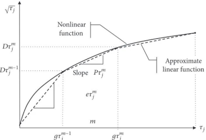
Figure 3: Piecewise linear functionPLFofWIC.

cost, the order quantity at each plant can be calculated using (2). Using the results for variables𝛿_𝑗 as demands and𝜂_𝑗 as demand variances for plants, with their corresponding values for the lead time and service level factor, the reorder point at each plant can be calculated using (5). The same can be done for warehouses using the values of𝜆_𝑘as demands and𝜋_𝑘as demand variances.

3.2.2. Linear Approximation of the Objective Function. This section presents a linear approximation approach for the safety stock costsSSCand working inventory costsWIC.WIC

in plant𝑗is calculated as_√𝜏_𝑗, as derived from (3) and (16). The approximation is based on a piecewise linear function (PLF) defined by two or more straight-lines, presented in different sections of the domain of the function as shown in Figure 3.

Considering a partition of𝜏_𝑗in𝑀sections, the function

√𝜏𝑗is approximated linearly by the expression𝐷𝜏𝑗𝑚−1⋅ 𝑒𝜏𝑚𝑗 + piecewise linear function of_√𝜏_𝑗is used or 0 otherwise. Also,

𝑓𝜏𝑚

𝑗 = 𝜏𝑗−𝑔𝜏𝑗𝑚−1are the units of𝜏𝑗in any point along section

𝑚.

The linear approximation ofWICat each plant is given by

(9)

Table 1: Parameters of the base case, associated with suppliers𝑖.

Parameter 𝑖 = 1 𝑖 = 2 𝑖 = 3 𝑖 = 4 𝑖 = 5 𝑖 = 6 𝑖 = 7 𝑖 = 8 𝑖 = 9 𝑖 = 10

𝑐𝑠_𝑖= 85 70 90 80 75 65 70 71 66 66

𝑈𝐶𝑠

𝑖= 30 28 30 28 24 25 28 21 28 30

Table 2: Parameters of the base case, associated with plants𝑗, and warehouses𝑘.

Plant 𝑗 = 1 𝑗 = 2 𝑗 = 3 Warehouse 𝑘 = 1 𝑘 = 2 𝑘 = 3 𝑘 = 4 𝑘 = 5

𝑐𝑝_𝑗= 150 200 110 𝑐𝑤_𝑘= 70 80 75 70 85

𝐹𝐶𝑝_𝑗= 187500 250000 137500 𝐹𝐶𝑤_𝑘= 131250 150000 97500 131250 121875

𝐻𝐶𝑝_𝑗 = 167 134 164 𝐻𝐶𝑤_𝑘 = 184 220 190 189 205

𝐿𝑇𝑝_𝑗 = 1 3 2 𝐿𝑇𝑤_𝑘 = 2 1 2 1 2

𝑂𝐶𝑝

𝑗= 646 657 656 𝑂𝐶𝑤𝑘 = 743 850 552 743 690

Table 3: Parameters of the base case, demand, and variance of retailers𝑙.

Retailer 𝑙 = 1 𝑙 = 2 𝑙 = 3 𝑙 = 4 𝑙 = 5 𝑙 = 6 𝑙 = 7 𝑙 = 8 𝑙 = 9 𝑙 = 10 𝑙 = 11 𝑙 = 12 𝑙 = 13

Demand (𝑑_𝑙) = 5 10 10 6 8 5 13 23 12 10 6 7 20

Variance (𝑢_𝑙) = 46 40 25 30 87 50 55 65 30 68 70 76 30

Retailer 𝑙 = 14 𝑙 = 15 𝑙 = 16 𝑙 = 17 𝑙 = 18 𝑙 = 19 𝑙 = 20 𝑙 = 21 𝑙 = 22 𝑙 = 23 𝑙 = 24 𝑙 = 25

Demand (𝑑_𝑙) = 10 20 9 17 15 15 24 5 25 23 16 14

Variance (𝑢_𝑙) = 35 86 40 50 25 10 60 68 40 73 45 50

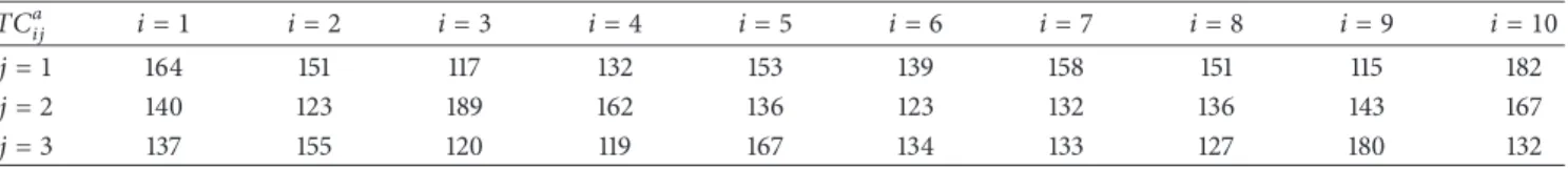
Table 4: Parameters of the base case, transportation unit cost from supplier𝑖to plant𝑗.

𝑇𝐶𝑎

𝑖𝑗 𝑖 = 1 𝑖 = 2 𝑖 = 3 𝑖 = 4 𝑖 = 5 𝑖 = 6 𝑖 = 7 𝑖 = 8 𝑖 = 9 𝑖 = 10

𝑗 = 1 164 151 117 132 153 139 158 151 115 182

𝑗 = 2 140 123 189 162 136 123 132 136 143 167

𝑗 = 3 137 155 120 119 167 134 133 127 180 132

|𝑀|

∑

𝑚=1

𝑒𝜏_𝑗𝑚= 𝑦_𝑗, ∀𝑗 = 1, . . . |𝐽| , (34)

𝑒𝜏_𝑗𝑚, 𝑦_𝑗∈ {0, 1} ,

𝑓𝜏_𝑗𝑚≥ 0,

∀𝑗 = 1, . . . |𝐽| , ∀𝑚 = 1, . . . |𝑀| .

(35)

Equation (31) represents the linear approximation of the

WIC at plant 𝑗. Equation (32) ensures that the average demand in plant𝑗is considered for the linear approximation. Equation (33) establishes that only a section𝑚must be used in the linear approximation. Equation (34) guarantees that the linear approximation is carried out only in open plants. Finally, (35) describes the domain of the variables. The same analysis is considered to generate the linear approximation of

SSCin each plant andWICandSSCin each warehouse. An alternative objective function Z1’ is defined. Z1’ is equivalent to Z1 but considering the linear approximation ofWICand SSCintroduced before. The new optimization model, with objective function Z1’ and all the linearized constraints, is named 4EILP-SS-L.

Table 5: Parameters of the base case, transportation unit cost from plant𝑗to warehouse𝑘.

𝑇𝐶𝑏

𝑗𝑘 𝑘 = 1 𝑘 = 2 𝑘 = 3 𝑘 = 4 𝑘 = 5

𝑗 = 1 164 140 137 132 162

𝑗 = 2 151 123 155 153 136

𝑗 = 3 117 189 120 119 167

4. Results and Discussion

In this section, five instance sizes with 10 cases each one are presented. The code of the instance size indicates the number of suppliers followed by the number of potential plants, followed by the number of potential warehouses, and the number of retailers. For example, instance size 5-3-5-10 indicates 5 suppliers, 3 potential plants, 5 potential warehouses, and 10 retailers.

(10)

557936

Group 1 (5-3-5-10) Group 2 (5-3-5-15) Group 3 (7-3-5-20) Group 4 (10-3-5-20) Group 5 (10-3-5-25)

A

Figure 4: Average total cost, comparing the nonlinear versus the linear models.

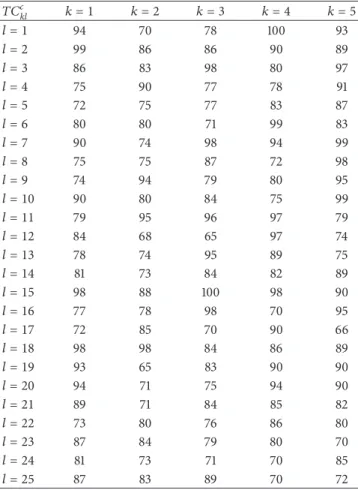
Table 6: Parameters of the base case, transportation unit cost from warehouses𝑘to retailer𝑙.

𝑇𝐶𝑐

base case, which were varied to construct the different cases. The case base has 10 potential suppliers, 3 potential plants, 5 potential warehouses, and 25 potential retailers. For example, to generate one instance of the size 5-3-5-10, 5 out of the 10 available suppliers in the base case were selected randomly, the 3 plants are used, the 5 warehouses are used, and 10 out of the 25 retailers were selected randomly from the base case. To generate one instance of the size 7-3-5-20, 7 out of the 10 available suppliers in the base case were selected randomly, the 3 plants are used, the 5 warehouses are used, and 20

out of the 25 retailers were selected randomly from the base case.

The uncertainty in demand is represented by the variance values shown in Table 3. In all the instances of the linear model, four intervals were used for the linearization, follow-ing the results from Diabat and Theodorou [44].

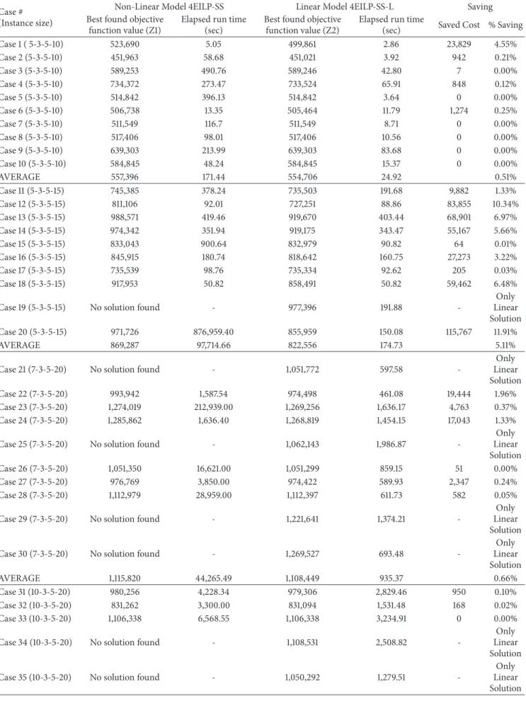
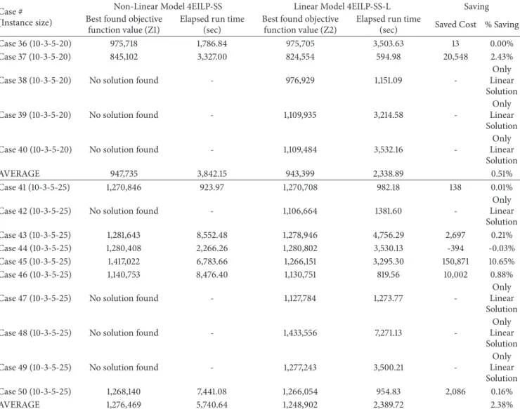
Table 7 shows the computational results of applying the nonlinear and the linear model with a service level of 95% (ZT_(0.95)= 1.64). Table 7 shows the objective function value Z1, the saved cost from the comparison, the % saving with respect to the solution of the nonlinear model, the run elapsed time for the solution with the linear model, and the cases where the solution was obtained only with the linear model. The comparison denotes the significant benefit (% Saving) that can be obtained by using the linear model instead of the nonlinear model. In this study, the average elapsed run time from the solutions of the linear model was set as a time limit on each group of instances when solving the nonlinear model. In the last column in Table 7, the cases where the nonlinear model does not converge (in the time limit) are shown as well. In order to make a fair comparison between both models, the total cost Z2 was obtained by using the values of the solution obtained by the linear model that optimizes Z1’ but evaluated in the original objective function Z1. Let X’ be the optimal solution of 4EILP-SS-L, then Z2 = Z1 (X’).

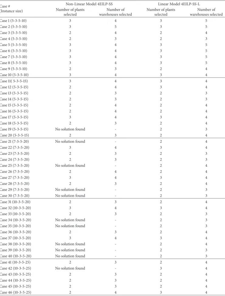
Table 8 shows the structure of the supply chain according to the results obtained with the models. In many cases, the structures are very similar, but the assignments between customers and warehouses, warehouses and plants, and flows from suppliers produced the differences in costs.

Figure 4 shows the comparison of the average total cost of the nonlinear and the linear models, where a solution was found. In all cases, the solutions of the linear model are cheaper than the solutions from the nonlinear model. The range of the average percent savings (% saving) is from 0.51% to 5.11%. The results of the nonlinear model may be better using a more efficient nonlinear optimizer, especially for the small instances, but it is expected that the linear model will be more efficient for larger instances.

(11)

Table 7: Results of applying the nonlinear model and the linear model considering a service level of 95%.

Case # (Instance size)

Non-Linear Model 4EILP-SS Linear Model 4EILP-SS-L Saving Best found objective

function value (Z1)

Elapsed run time (sec)

Best found objective function value (Z2)

Elapsed run time

(sec) Saved Cost % Saving

Case 1 ( 5-3-5-10) 523,690 5.05 499,861 2.86 23,829 4.55%

Case 2 (5-3-5-10) 451,963 58.68 451,021 3.92 942 0.21%

Case 3 (5-3-5-10) 589,253 490.76 589,246 42.80 7 0.00%

Case 4 (5-3-5-10) 734,372 273.47 733,524 65.91 848 0.12%

Case 5 (5-3-5-10) 514,842 396.13 514,842 3.64 0 0.00%

Case 6 (5-3-5-10) 506,738 13.35 505,464 11.79 1,274 0.25%

Case 7 (5-3-5-10) 511,549 116.7 511,549 8.71 0 0.00%

Case 8 (5-3-5-10) 517,406 98.01 517,406 10.56 0 0.00%

Case 9 (5-3-5-10) 639,303 213.99 639,303 83.68 0 0.00%

Case 10 (5-3-5-10) 584,845 48.24 584,845 15.37 0 0.00%

AVERAGE 557,396 171.44 554,706 24.92 0.51%

Case 11 (5-3-5-15) 745,385 378.24 735,503 191.68 9,882 1.33%

Case 12 (5-3-5-15) 811,106 92.01 727,251 88.86 83,855 10.34%

Case 13 (5-3-5-15) 988,571 419.46 919,670 403.44 68,901 6.97%

Case 14 (5-3-5-15) 974,342 351.94 919,175 343.47 55,167 5.66%

Case 15 (5-3-5-15) 833,043 900.64 832,979 90.82 64 0.01%

Case 16 (5-3-5-15) 845,915 180.74 818,642 160.75 27,273 3.22%

Case 17 (5-3-5-15) 735,539 98.76 735,334 92.62 205 0.03%

Case 18 (5-3-5-15) 917,953 50.82 858,491 50.82 59,462 6.48%

Case 19 (5-3-5-15) No solution found - 977,396 191.88

-Only Linear Solution

Case 20 (5-3-5-15) 971,726 876,959.40 855,959 150.08 115,767 11.91%

AVERAGE 869,287 97,714.66 822,556 174.73 5.11%

Case 21 (7-3-5-20) No solution found - 1,051,772 597.58

Case 22 (7-3-5-20) 993,942 1,587.54 974,498 461.08 19,444 1.96%

Case 23 (7-3-5-20) 1,274,019 212,939.00 1,269,256 1,636.17 4,763 0.37%

Case 24 (7-3-5-20) 1,285,862 1,636.40 1,268,819 1,454.15 17,043 1.33%

Case 25 (7-3-5-20) No solution found - 1,062,143 1,986.87

Case 26 (7-3-5-20) 1,051,350 16,621.00 1,051,299 859.15 51 0.00%

Case 27 (7-3-5-20) 976,769 3,850.00 974,422 589.93 2,347 0.24%

Case 28 (7-3-5-20) 1,112,979 28,959.00 1,112,397 611.73 582 0.05%

AVERAGE 1,115,820 44,265.49 1,108,449 935.37 0.66%

Case 31 (10-3-5-20) 980,256 4,228.34 979,306 2,829.46 950 0.10%

Case 32 (10-3-5-20) 831,262 3,300.00 831,094 1,531.48 168 0.02%

Case 33 (10-3-5-20) 1,106,338 6,568.55 1,106,338 3,234.91 0 0.00%

(12)

Table 7: Continued.

Non-Linear Model 4EILP-SS Linear Model 4EILP-SS-L Saving Best found objective

function value (Z1)

Elapsed run time (sec)

Best found objective function value (Z2)

Elapsed run time

(sec) Saved Cost % Saving

Case 36 (10-3-5-20) 975,718 1,786.84 975,705 3,503.63 13 0.00%

Case 37 (10-3-5-20) 845,102 3,327.00 824,554 594.98 20,548 2.43%

Case 38 (10-3-5-20) No solution found - 976,929 1,151.09

AVERAGE 947,735 3,842.15 943,399 2,338.89 0.51%

Case 41 (10-3-5-25) 1,270,846 923.97 1,270,708 982.18 138 0.01%

Case 43 (10-3-5-25) 1,281,643 8,552.48 1,278,946 4,756.29 2,697 0.21%

Case 44 (10-3-5-25) 1,280,408 2,266.26 1,280,802 3,530.13 -394 -0.03%

Case 45 (10-3-5-25) 1,417,022 6,783.66 1,266,151 3,295.30 150,871 10.65%

Case 46 (10-3-5-25) 1,140,753 8,476.40 1,130,751 819.56 10,002 0.88%

Case 50 (10-3-5-25) 1,268,140 7,441.08 1,266,054 954.83 2,086 0.16%

AVERAGE 1,276,469 5,740.64 1,248,902 2,389.72 2.38%

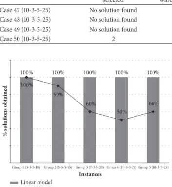
of performance of the nonlinear model goes from 50% to 100% among the instances. Using the linear model an optimal solution was obtained in all cases. For these instance sizes, one can be confident in obtaining a good solution with the linear model, which is not the case with the nonlinear model.

5. Conclusions and Final Remarks

This research introduced an inventory-location model, 4EILP-SS, for the network design of a four-echelon supply chain, considering the location of warehouses and plants, transportation cost, inventory costs, and supplier selection. The inventory policy and network design decisions are tactical and strategic decisions that should be analyzed con-currently. This is attained using the aforementioned model. This model can be applied to design complex and long supply chains, like in the automotive industry because of the offshore movement of production facilities from indus-trialized countries to emerging economies. In many cases, there is infrastructure available in the country, and it is easy to adapt the model to that situation fixing locations for the

available facilities and allowing the model to decide for the new optimum flows and locations of new facilities.

The model proposed becomes nonlinear because of the application of the continuous review inventory policy. This feature added to the computational complexity inherited from the Facility Location Problem makes the problem hard to solve. The mixed integer nonlinear model was reformu-lated using a piecewise linear function and a reformulation of nonlinear constraints in order to generate a mixed integer linear model. Several instances were solved using the linear and nonlinear models, comparing the results in terms of cost savings, number of solutions obtained, and computa-tional runtime. It was observed that solving the nonlinear model with the commercial software generated local optimal solutions, and in several cases the software either did not converge or resulted in infeasible solutions. The total cost of the original objective function is lower, in most of the cases, with the solution obtained by the linear model than the solution obtained by the nonlinear model.

(13)

Table 8: Structure of the supply chain applying the nonlinear model and the linear model considering a service level of 95%.

Non-Linear Model 4EILP-SS Linear Model 4EILP-SS-L Number of plants

selected

Number of warehouses selected

Number of plants selected

Number of warehouses selected

Case 1 (5-3-5-10) 3 4 3 5

Case 2 (5-3-5-10) 3 5 3 5

Case 3 (5-3-5-10) 2 4 2 4

Case 4 (5-3-5-10) 2 3 2 3

Case 5 (5-3-5-10) 3 4 3 5

Case 6 (5-3-5-10) 3 4 3 5

Case 7 (5-3-5-10) 3 4 3 5

Case 8 (5-3-5-10) 3 4 3 5

Case 9 (5-3-5-10) 2 3 2 4

Case 10 (5-3-5-10) 3 4 3 4

Case 11( 5-3-5-15) 3 4 3 4

Case 12 (5-3-5-15) 2 4 3 4

Case 13 (5-3-5-15) 2 3 2 3

Case 14 (5-3-5-15) 2 3 2 3

Case 15 (5-3-5-15) 2 4 2 4

Case 16 (5-3-5-15) 2 4 2 4

Case 17 (5-3-5-15) 3 4 3 4

Case 18 (5-3-5-15) 2 3 2 4

Case 19 (5-3-5-15) No solution found - 2 3

Case 20 (5-3-5-15) 2 3 2 4

Case 22 (7-3-5-20) 3 4 3 4

Case 23 (7-3-5-20) 2 3 2 3

Case 24 (7-3-5-20) 2 3 2 3

Case 26 (7-3-5-20) 2 4 2 4

Case 27 (7-3-5-20) 3 4 3 4

Case 28 (7-3-5-20) 2 3 2 4

Case 31 (10-3-5-20) 2 3 2 4

Case 32 (10-3-5-20) 3 4 3 4

Case 33 (10-3-5-20) 2 3 2 3

Case 36 (10-3-5-20) 2 3 2 4

Case 37 (10-3-5-20) 3 4 3 4

Case 41 (10-3-5-25) 2 3 2 4

Case 43 (10-3-5-25) 2 3 2 4

Case 44 (10-3-5-25) 2 3 2 4

Case 45 (10-3-5-25) 2 3 2 4

(14)

Table 8: Continued.

Non-Linear Model 4EILP-SS Linear Model 4EILP-SS-L Number of plants

Case 50 (10-3-5-25) 2 3 2 4

100% 100% 100% 100% 100%

100%

90%

60%

50%

60%

Group 1 (5-3-5-10) Group 2 (5-3-5-15) Group 3 (7-3-5-20) Group 4 (10-3-5-20) Group 5 (10-3-5-25)

Linear model

Figure 5: Percent of solutions obtained, comparing nonlinear versus linear models.

supply chain, where facility location and inventory man-agement decisions are considered in two stages (plants and warehouses), and transportation or assignment decisions are modeled in three stages of the supply chain, i.e., suppliers-plants, plants-warehouses, and warehouses-customers. Sec-ondly, a linearization approach of the proposed nonlinear model, in order to facilitate its applicability and its effective and efficient implementation, improves both solutions qual-ity and computational times.

The proposed linear model proves to be useful for decision makers interested in analyzing and designing supply chain networks with the structure of a 4EILP-SS. The problem can be analyzed and solved in a short period of time and with significant confidence in the solution quality.

The experiments conducted allowed us to understand the complexity of the problem. For this study, LINGO was used to solve the linear and the nonlinear models, but future work may take advantage of using more efficient commercial soft-ware to solve larger instances. As observed, using commercial optimizers may not be the best alternative when it comes to solve very large instances. Therefore, immediate future research should consider the development of other heuris-tics aimed to tackle large instances (Lagrangian relaxation, Bender decompositions, Cutting planes, and Metaheuristics). Another direction is to extend the pricing approach proposed by Shu et al. [18] to solve a similar problem to the long supply chain proposed in this paper.

In addition, a deeper study may involve the analysis of the relations between parameters like costs, capacities, lead times, and demand variability, to understand their impact in the supply chain network configuration.

Finally, it would be interesting to extend the model to analyze multiobjective situations, more common when designing supply chain networks for real situations.

Data Availability

The data used to support the findings of this study are available from the corresponding author upon request.

Conflicts of Interest

The authors declare that there are no conflicts of interest regarding the publication of this article.

Acknowledgments

This research was supported by Programa para el Mejoramiento del Profesorado PROMEP (Grant ITESUR-001 Charter no. PROMEP/103.5/10/5709) and Universidad Panamericana (Grant no. UP-CI-2018-ING-GDL-06).

References

[1] M. Mourits and J. J. Evers, “Distribution network design: an integrated planning support framework,”Logistics Information Management, vol. 9, pp. 45–54, 1995.

[2] R. Z. Farahani, H. Rashidi Bajgan, B. Fahimnia, and M. Kaviani, “Location-inventory problem in supply chains: A modelling review,”International Journal of Production Research, vol. 53, no. 12, pp. 3769–3788, 2015.

[3] OICA, International Organization of Motor Vehicle Man-ufacturers, Production statistics, 2017, http://www.oica.net/ category/production-statistics/2017-statistics/.

[4] H. Hamacher and Z. Drezner,Facility Location: Applications and Theory, Springer, Berlin, Germany, 2002.

[5] M. S. Daskin, Network and Discrete Location: Models, Algo-rithms, and Applications, Wiley-Interscience, New York, NY, USA, 1st edition, 1995.

[6] S. Nickel and J. Puerto,Location Theory: A Unified Approach, Springer, New York, NY, USA, 2005.

(15)

[8] H. A. Eiselt and V. Marianov,Foundations of Location Analysis, Springer, New York, NY, USA, 2011.

[9] H. A. Eiselt and V. Marianov,Applications of Location Analysis, Springer, New York, NY, USA, 2015.

[10] V. Jayaraman, “Transportation, facility location and inventory issues in distribution network design: An investigation,” Inter-national Journal of Operations and Production Management, vol. 18, no. 5, pp. 471–494, 1998.

[11] L. K. Nozick and M. A. Turnquist, “Integrating inventory impacts into a fixed-charge model for locating distribution centers,”Transportation Research Part E: Logistics and Trans-portation Review, vol. 34, no. 3, pp. 173–186, 1998.

[12] S. J. Erlebacher and R. D. Meller, “The interaction of location and inventory in designing distribution systems,”IIE Transac-tions, vol. 32, no. 2, pp. 155–166, 2000.

[13] L. K. Nozick and M. A. Turnquist, “A two-echelon inventory allocation and distribution center location analysis,” Trans-portation Research Part E: Logistics and TransTrans-portation Review, vol. 37, no. 6, pp. 425–441, 2001.

[14] L. K. Nozick and M. A. Turnquist, “Inventory, transportation, service quality and the location of distribution centers,” Euro-pean Journal of Operational Research, vol. 129, no. 2, pp. 362–371, 2001.

[15] M. S. Daskin, C. R. Coullard, and Z. J. M. Shen, “An inventory-location model: formulation, solution algorithm and computa-tional results,”Annals of Operations Research, vol. 110, pp. 83– 106, 2002.

[16] Z.-J. M. Shen, C. R. Coullard, and M. S. Daskin, “A joint location-inventory model,”Transportation Science, vol. 37, no. 1, pp. 40–55, 2003.

[17] P. A. Miranda and R. A. Garrido, “Incorporating inventory control decisions into a strategic distribution network design model with stochastic demand,”Transportation Research Part E: Logistics and Transportation Review, vol. 40, no. 3, pp. 183–207, 2004.

[18] J. Shu, C.-P. Teo, and Z. M. Shen, “Stochastic transportation-inventory network design problem,”Operations Research, vol. 53, no. 1, pp. 48–60, 2005.

[19] L. V. Snyder, M. S. Daskin, and C.-P. Teo, “The stochastic loca-tion model with risk pooling,”European Journal of Operational Research, vol. 179, no. 3, pp. 1221–1238, 2007.

[20] J. Shu, Q. Ma, and S. Li, “Integrated location and two-echelon inventory network design under uncertainty,”Annals of Opera-tions Research, vol. 181, pp. 233–247, 2010.

[21] P. A. Miranda and R. A. Garrido, “A simultaneous inventory control and facility location model with stochastic capacity constraints,”Networks and Spatial Economics, vol. 6, no. 1, pp. 39–53, 2006.

[22] P. A. Miranda and R. A. Garrido, “Valid inequalities for Lagrangian relaxation in an inventory location problem with stochastic capacity,”Transportation Research Part E: Logistics and Transportation Review, vol. 44, no. 1, pp. 47–65, 2008. [23] L. Ozsen, C. R. Coullard, and M. S. Daskin, “Capacitated

warehouse location model with risk pooling,”Naval Research Logistics (NRL), vol. 55, no. 4, pp. 295–312, 2008.

[24] P. A. Miranda and G. Cabrera, “Inventory location problem with stochastic capacity constraints under periodic review(R, s, S),” inProceedings of the International Conference on Industrial Logistics: Logistics and Sustainability, (ICIL ’10), pp. 289–296, 2010.

[25] G. Cabrera, P. A. Miranda, E. Cabrera et al., “Solving a novel inventory location model with stochastic constraints and inven-tory control policy,”Mathematical Problems in Engineering, vol. 2013, Article ID 670528, 12 pages, 2013.

[26] J.-H. Kang and Y.-D. Kim, “Inventory control in a two-level supply chain with risk pooling effect,”International Journal of Production Economics, vol. 135, no. 1, pp. 116–124, 2012. [27] F. Silva and L. Gao, “A joint replenishment inventory-location

model,”Networks and Spatial Economics, vol. 13, no. 1, pp. 107– 122, 2013.

[28] J.-S. Tancrez, J.-C. Lange, and P. Semal, “A location-inventory model for large three-level supply chains,” Transportation Research Part E: Logistics and Transportation Review, vol. 48, no. 2, pp. 485–502, 2012.

[29] A. Diabat, J.-P. Richard, and C. . Codrington, “A Lagrangian relaxation approach to simultaneous strategic and tactical planning in supply chain design,”Annals of Operations Research, vol. 203, pp. 55–80, 2013.

[30] M. Shahabi, S. Akbarinasaji, A. Unnikrishnan, and R. James, “Integrated inventory control and facility location decisions in a multi-echelon supply chain network with hubs,”Networks and Spatial Economics, vol. 13, pp. 497–514, 2013.

[31] Z.-J. M. Shen and M. S. Daskin, “Trade-offs between customer service and cost in integrated supply chain design,” Manufactur-ing and Service Operations Management, vol. 7, no. 3, pp. 188– 207, 2005.

[32] S. Gaur and A. R. Ravindran, “A bi-criteria model for the inventory aggregation problem under risk pooling,”Computers & Industrial Engineering, vol. 51, no. 3, pp. 482–501, 2006. [33] P. A. Miranda and R. A. Garrido, “Inventory service-level

optimization within distribution network design problem,”

International Journal of Production Economics, vol. 122, no. 1, pp. 276–285, 2009.

[34] H.-Y. Mak and Z. M. Shen, “A two-echelon inventory-location problem with service considerations,”Naval Research Logistics (NRL), vol. 56, no. 8, pp. 730–744, 2009.

[35] P. Escalona, F. Ord´o˜nez, and V. Marianov, “Joint location-inventory problem with differentiated service levels using crit-ical level policy,”Transportation Research Part E: Logistics and Transportation Review, vol. 83, pp. 141–157, 2015.

[36] A. Atamt¨urk, G. Berenguer, and Z.-J. Shen, “A conic integer programming approach to stochastic joint location-inventory problems,”Operations Research, vol. 60, no. 2, pp. 366–381, 2012. [37] O. Kaya and B. Urek, “A mixed integer nonlinear programming model and heuristic solutions for location, inventory and pricing decisions in a closed loop supply chain,”Computers & Operations Research, vol. 65, pp. 93–103, 2016.

[38] M. a. Schuster Puga and J.-S. Tancrez, “A heuristic algorithm for solving large location-inventory problems with demand uncertainty,”European Journal of Operational Research, vol. 259, no. 2, pp. 413–423, 2017.

[39] P. Escalona, V. Marianov, F. Ord´o˜nez, and R. Stegmaier, “On the effect of inventory policies on distribution network design with several demand classes,”Transportation Research Part E: Logistics and Transportation Review, vol. 111, pp. 229–240, 2018. [40] F. J. Tapia-Ubeda, P. A. Miranda, and M. Macchi, “A generalized Benders decomposition based algorithm for an inventory loca-tion problem with stochastic inventory capacity constraints,”

(16)

[41] R. E. Perez Loaiza, E. Olivares-Benitez, P. A. Miranda Gonzalez, A. Guerrero Campanur, and J. L. Martinez Flores, “Supply chain network design with efficiency, location, and inventory policy using a multiobjective evolutionary algorithm,” International Transactions in Operational Research, vol. 24, no. 1-2, pp. 251– 275, 2017.

[42] F. You and I. E. Grossmann, “Integrated multi-echelon supply chain design with inventories under uncertainty: MINLP mod-els, computational strategies,”AIChE Journal, vol. 56, no. 2, pp. 419–440, 2010.

[43] K. Petridis, “Optimal design of multi-echelon supply chain networks under normally distributed demand,”Annals of Oper-ations Research, vol. 227, no. 1, pp. 63–91, 2015.

[44] A. Diabat and E. Theodorou, “A location-inventory supply chain problem: Reformulation and piecewise linearization,”

Computers & Industrial Engineering, vol. 90, pp. 381–389, 2015. [45] A. Nyberg, I. E. Grossmann, and T. Westerlund, “An efficient

(17)

Hindawi

www.hindawi.com Volume 2018

Mathematics

Journal of

Hindawi

Mathematical Problems in Engineering Applied Mathematics Hindawi

Probability and Statistics Hindawi

Hindawi

Mathematical PhysicsAdvances in

Complex Analysis

Journal of

Hindawi

Optimization

Journal of

Hindawi

Engineering Mathematics International Journal of

Hindawi

Operations Research

Journal of

Hindawi

Function Spaces

Abstract and Applied Analysis Hindawi

International Journal of Mathematics and Mathematical Sciences

Hindawi

Hindawi Publishing Corporation

http://www.hindawi.com Volume 2013

Hindawi www.hindawi.com

World Journal

Volume 2018

Numerical Analysis

Discrete Dynamics in Nature and Society

Hindawi

Hindawi www.hindawi.com

Differential Equations International Journal of

Volume 2018

Hindawi

Decision Sciences

Hindawi

Analysis

International Journal of

Hindawi

Stochastic Analysis

International Journal of

Design of a Logistics Nonlinear System for a Complex, Multiechelon, Supply Chain Network with Uncertain Demands

Research Article