Derivation and application of the stream of variation model to the manufacture of ceramic floor tiles

Texto completo

(1)Derivation and application of the Stream of Variation Model to the Manufacture of Ceramic Floor Tiles Jose V. Abellan-Nebot1 Dpto. Ing. Sistemas Industriales y Diseño, Universitat Jaume I, 12006, Castellón de la Plana, Spain [email protected] One of the main problems in the manufacture of floor tiles is the dimensional variability of the ceramic product, which leads to the product having to be classified into different dimensional qualities with an increase in cost. In this paper we propose a novel way of modelling the dimensional variability of ceramic floor tiles by the adaptation of the Stream of Variation model. The proposed methodology and its potential applicability contributes to the integration of process knowledge in the ceramic tile industry and allow tile manufacturers have a new methodology for process improvement, variation reduction and dimensional control. Keywords: ceramic tiles; stream-of-variation; dimensional variability; multi-stage manufacturing systems. 1. Introduction Companies dedicated to the manufacture of ceramic floor tiles classify the final product according to its size in order to avoid problems arising from a lack of dimensional uniformity when the customer is laying the tiles. The tiles are classified by establishing a series of sizes, usually called calibers, each of which has its own margin of variation or tolerance that depends on the quality standards set by the company. One of the most important problems for the ceramic floor tile manufacturing sector is the difficulty involved in achieving production batches with pieces of the same size or caliber (Mallol et al. 2012). In a recent survey (Bonavia and Marin 2006), it was shown that an average of 89% of the ceramic tile production is within a prime quality standard, whereas the rest of the tile production falls within secondary and tertiary quality levels, i.e. it has different calibers. This problem entails a rise in cost due to the increase in space required in the warehouse, the logistic complexity involved in managing stock separated into different calibers, the need to oversize manufacturing batches and, very often, complaints from customers about.

(2) dimensional variations. Unlike other manufacturing industries, the inherent variability of the ceramic tile manufacturing process complicates an efficient dimensional quality control. Quality control was initiated in 1924 by W.A. Shewhart who suggested the use of control charts as a tool to monitor and control production processes with the objective of improving quality. The American statistician W.E. Deming promoted the application of quality control techniques in Japan after the Second World War which supposed a significant contribution to Japan’s reputation for innovative high-quality products and its emergence as an economic power. A step forward in quality control was defined as quality assurance, which was started to be adopted by advanced manufacturing companies in 1960. The purpose of quality assurance is the conformance of products, services and processes with given requirements and standards through systematic measurement, control and analysis of performance to detect special causes of variations and achieve process standardization (Jabnoun, 2002). In 1957 S.J. Morrison presented a method for variance transmission where each variable contribution to the product variability is estimated by applying an error transmission formula. This idea of variance transmission was an early exposition of design robustness and preceded the work that Genichi Taguchi conducted decades later. In the eighties, the development of the Theory of Constraints by E.M.Goldratt also dealt with the influence of variation in processing and material transfer times on throughput and inventory and proved the importance of considering every complex system, including manufacturing processes, as multiple linked activities, one of which acts as a constraint upon the entire system. At the end of the nineties, a renew interest of the problem of variation and its propagation in manufacturing systems was arisen and a new approach called the Stream of Variation (SoV) model was developed. This model was firstly derived by Jin and Shi (1999) for dimensional control in multi-stage assembly processes using the state space modelling approach commonly applied in control systems. The model was adapted for multi-stage machining systems by Zhou et al. (2003) where sources of error such as those related to fixture, datums and machining were included and it was later expanded by Abellan-Nebot et al. (2012b) to include different machining errors. The.

(3) applicability of the model has been successfully tested in many different fields such as fault diagnosis (Ding et al. 2002; Ding et al. 2003), manufacturing tolerance process allocation (AbellanNebot et al 2013; Chen et al. 2006; Loose et al. 2010), dimensional control (Abellan-Nebot at al 2012a) and process planning (Abellan-Nebot et al 2012c). However, despite the success of the SoV model, this approach has been mainly applied in discrete manufacturing systems where the relationships between dimensional deviations and sources of error can be derived by kinematic equations. In the ceramic tile industry, several studies have attempted to model the overall manufacturing process for the purpose of analysing the interrelation among the different variables throughout different stages and identifying the causes of dimensional variability. Among the most significant studies, De Noni et al. (2006) proposed a model based on a Taylor series expansion in order to determine the influence of the different process variables on the final dimensions of the tiles being fired. The variables considered in the model were the size distribution and moisture content of the spray-dried powder, compaction pressure, extraction time, mass of the tile and maximum firing temperature. The coefficients of the Taylor series were adjusted by means of polynomial regressions, and in a subsequent analysis it was shown that the variations in the mass of the tile, the maximum firing temperature and the moisture content of the spray-dried powder are, in that order, the main causes of dimensional variation in the process studied. Yet, the model does not take into account the possible correlation of the process variables and neither does it present a structure that defines the contribution of the variability in each stage with its interrelation with the ensuing stages, which makes it difficult to apply for process improvement. Similar studies were proposed in (Heredia and Gras 2011; Heredia and Gras 2010), where each stage is defined by a first-order autoregressive model that is adjusted by experimentation or using historical data. A subsequent analysis of variance makes it possible to quantify the influence of each of the process variables on the final propagation. Thus, in the case of the study presented, it was found that 42% of the dimensional variability was due to variations in the moisture content, 16% owing to the.

(4) composition of the material and 16% as a result of the temperature gradients that existed in the firing kiln, among others. Santos Barbosa et al. (2013) also attempted to determine how the influence of the process variables at each stage is related to the intermediate and final dimensions of the tile. However, despite being the first clear attempt to identify the whole process as an interrelated multi-stage system, mathematically it does not define a global equation where the final dimension of the floor tile is related to all process variables and basically remains a single-stage model obtained in different stages of the process. Furthermore, these previous modelling approaches overlooked the potential applicability of a global model of the manufacturing process in terms of fault diagnosis, compensability (real time control of dimensional quality) and tolerance process allocation. This paper presents a novel way of modelling the dimensional variability of ceramic floor tiles by a new methodology based on the SoV model adapted to deal with a continuous production. To the best of our knowledge, this is the first attempt to model the floor tile manufacturing process using this multi-stage modelling approach for quality improvement. The potential applicability of this model, such as detection of critical stages that contributes the most to dimensional variability, feed-forward control for dimensional variation reduction and monitoring and fault detection, among others, are briefly described and illustrated by a case study. The paper is organised as follows. Section 2 gives a brief overview of the manufacturing process of ceramic floor tiles and the critical process variables that influence on dimensional variability. Section 3 presents the Stream of Variation approach and its adaptation, stage by stage, for modelling the manufacturing process of ceramic tiles. Section 4 shows the potential applicability of the model for quality improvement, feed-forward control, monitoring and fault detection. Finally, Section 5 illustrates a case study and Section 6 shows the conclusions of the research.. 2. Floor tile manufacturing process and process variables The floor tile manufacturing process starts with the mixing of a specific formulation of raw materials in a ball mill, which runs in continuous operation. The solids mixed with approximately.

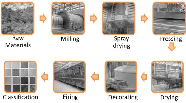
(5) 35% water are introduced into one side of the mill together with a deflocculant additive (polyphosphates and others), which helps to keep them in suspension while also controlling the viscosity, and a charge of silex or alumina balls is used to grind the material. The ground product is obtained at the other end of the mill in the form of a suspension, usually known as slip or slurry. The slurry is injected at high pressure by hydraulic pumps into the spray dryer where the moisture contained in the slurry evaporates and granular powders are obtained with a suitable particle size. The granular material, with a moisture content of between 5% and 7%, is discharged onto a conveyor belt and taken to silos. The spray-dried powder is then poured into mould cavities with the proper floor tile format. The aim of this stage, called the pressing stage, is to press the powder in order to obtain the shape of the tile with the maximum raw apparent/bulk density (compaction) of the body that will allow optimal sintering. From the pressing stage, the tiles move on to the drying and decorating stages, where they are dried and glazed. The following stage is firing, where the tiles are introduced into kilns for sintering. After the firing cycle, the resulting tiles present mechanical, chemical and dimensional characteristics in accordance with the desired specifications, and a final stage of inspection and packaging ends the manufacturing process. The complete manufacturing process is illustrated in Figure 1.. Classification. Firing. Decorating. Figure 1. Stages in the process of manufacturing ceramic floor tiles.. Drying.

(6) The process of manufacturing ceramic floor tiles has been widely analysed in the literature and a large number of studies have experimentally investigated the process variables that affect each stage of the process, as well as those that are known to play a significant role in determining the final dimensional quality. In Escardino et al. (1981), the authors reported the importance of the mineral composition of the raw materials used in relation to the dimensional stability and the water absorption. Several combinations of raw materials with different percentages of feldspar, quartz and different types of clay were tested and a clear influence of composition on linear contraction and range of firing temperatures was observed. In porcelain floor tiles, where plastic ball clays, kaolin, feldspar-quartz raw materials and pure quartz sand are commonly used, the ball clays are known to be the raw material with the largest qualitative variability (Galos 2011, Andreola et al. 2009). Other research works were focused on the milling stage. In Blasco et al. (1982), the authors studied the optimum type and content of deflocculant to be added in order to minimise the apparent viscosity and obtain a more efficient process. A similar study was conducted by Barrachina et al. (2015), where it was analysed the effect of different deflocculants on the rheological properties of the ceramic slurry with special attention on the effect on viscosity. Mondragon et al. (2012) studied the influence of slurry characteristics, such as solid mass load, primary particle size, viscosity, flocculation state and surface tension, on the resulting morphology of the powder after spray drying. In their findings, the most significant effects that influence porosity and thus, the dimensional contraction after firing, were the primary particle size of the composition, the initial solid mass load and the flocculation state from milling. In Da Silva et al. (2008), the authors also studied the influence of the use of recycling water from the manufacturing process on the ceramic suspension viscosity under different percentages of deflocculants. At the spray drying stage, variations in the resulting grain size distribution, grain shapes and moisture content generate different levels of compaction after tile pressing, which will produce dimensional variations at the firing stage. As reported in Negre and Sánchez (1996), the moisture of.

(7) the particles depends on different parameters such as the outlet temperature, the inlet temperature, the feed viscosity, the pressure of the production system, the amount of chemicals used and also the solid content of the slurry in the spray drying process. The importance of controlling variations in the spray drying operation was analysed by Negre et al. (1994), who reported moisture variations as a key factor for floor tile dimensional control. Other factors, such as the shape and size of the grains previously obtained from the milling stage, were also reported as important factors in the performance of subsequent stages such as pressing and firing. Some researchers have focused their attention on the pressing stage in order to understand its influence on the dimensional variability of ceramic floor tiles. Poyatos et al. (2010) argued that the key parameter in the variability of the pieces after firing is the variability of the bulk/apparent density following pressing. In order to control this variability, they developed an integral control system for the pressing operation, whereby the pressure exerted by the press and the filling of each of the cavities are regulated according to the moisture content of the spray-dried powder that enters the press. In the firing stage, Jarque et al. (2002) studied the influence of the operating conditions of the roller kiln on the curvature of ceramic floor tiles. In that study it was shown that the curvature of the tiles was directly related to changes in the set-point temperature of the thermocouples and the existence of gaps between pieces throughout the kiln. Furthermore, it was observed that the control parameters in all the gas valves, set by default by the manufacturer of the kiln, gave rise to a continuous oscillation of the temperature that had a negative impact on the curvature of the tiles. In Ferrer et al. (1994), the temperature gradients between the middle region and the walls of the kiln were measured using specially designed rollers with sensors fitted transversally inside the kiln. The importance of this gradient temperature was reported as critical in Heredia and Gras (2011), explaining 16% of the final dimensional variations of floor tiles. From the literature it is clearly shown that process variables at each stage have an important impact on the performance of downstream stages in the manufacturing process of ceramic floor.

(8) tiles. As a result, the final product quality should be considered as a complex function of all the process variables, including the interrelation among the different variables in the different stages of the process.. 3. Derivation of the Stream of Variation Model The multi-stage modelling approach called the Stream of Variation (SoV) model is adapted here to model the propagation of errors throughout the process of manufacturing ceramic floor tiles and their influence on dimensional variability. For modelling purposes, we define the manufacturing process variables as controllable variables, manipulated variables and disturbance variables. Controllable variables refer to those variables that have to be controlled at each stage, e.g., the moisture content at the spray drying stage; manipulated variables are those variables that have an influence on the controllable variables and can be manipulated to modify process performance; and disturbance variables refer to those variables that may change continuously and are not controlled during the process. In multi-stage processes, the SoV model defines the product quality throughout the multiple manufacturing stages by the equation (Zhou et al. 2003):. where the vector xk contains the controllable variables in stage k, Ak-1 is a matrix that relates the variables to be controlled in stage k with those in stage k-1; uk is a vector with the manipulated variables in stage k; Bk is a matrix that shows this relationship; and wk indicates the modelling error. Moreover, the measurements after stage k are defined with the vector yk, and the measurement errors are represented by vk. Thus, the relationship between the real value xk and the measured value at stage k, yk, is:.

(9) Since single models applied at each stage are non-linear, these models have to be linearised around a functioning point in order to build the SoV model. Therefore, the variables presented in the SoV model will refer to deviations with respect to a functioning point. For the manufacturing process of ceramic tiles, the multi-stage process is defined by 4 stages: milling, spray drying, pressing and firing. A first stage related to the raw material formulation and the variations in chemical composition is not considered in this paper, and the drying and decoration stages are not included since they have no influence on the appearance of calibers and their influence is more related with defects in the tiles (e.g. pinholes, crazing and peeling). In the following subsections it is shown the main process variables and a linearization model for each stage. Note that the final SoV model is the result of the stacked models at each single stage as it is shown in Section 3.5.. 3.1. Milling The variables that should be controlled at this stage are density of the slurry (), viscosity () and grain size (κ) of the slurry particles. To control these variables, the manipulated variables are the flow rates of the solid (flowsolid), water (flowwater) and deflocculant (flowdefloc). In the process, the state of the balls (wear balls) used for grinding may be considered as a disturbance variable. Thus, the following equations can be defined: ;; where f(·), g(·), and h(·) are non-linear functions, and the variables are and . Assuming that the process behaves linearly when there are small variations around the working conditions {d0, e0}, these functions can be linearised through Taylor series expansion as:. Thus, the deviation from the working conditions is:. By linearisation, the resulting equations can be derived in a matrix form:.

(10) Considering disturbances and modelling errors all together since they are unknown. Denoting z1 = [∆, ∆, ∆κ]T, t1 = [∆flowsolid, ∆flowwater, ∆flowdefloc]T, l1 = [,,]T, and the Jacobian matrix as J1, the above equation is rewritten as:. At this stage, the density (), viscosity () and grain size () of the slurry particles are measured to control the process. Thus, the following equation is defined:. where m1 = [, , ]T, G1 = I (I is the identity matrix), and the measurement errors of the sensors applied are denoted as s1 = [,,]T. Note that G1 is the identity matrix if the three variables are measured. Otherwise, G1 should be modified to indicate which variables are being measured.. 3.2. Spray drying The controllable variables at this stage are the moisture content of the spray-dried powder (h) and its grain size (β). The manipulated variables are: the temperature of the air stream (Ta), the flow rate of incoming and outgoing dry air (flowin, flowout), the depression in the evaporation tower (d), the input pressure of the slurry (pslurry) and the slurry flow rate (flowslurry). Additionally, the outside temperature (Tout) may also be considered as a disturbance variable. From the previous stage, the density (∆), viscosity (∆) and grain size of the slurry (∆κ) will also influence the spray drying stage. Following the same procedure as shown above, after linearisation the following matrix expression is defined:. where z2 = [∆h, ∆β]T, t2 = [∆Ta, ∆flowin, ∆flowout, ∆d, ∆pslurry, ∆flowslurry]T, l2 = [lh, lβ]T, and K11 and J2 are the corresponding Jacobian matrices. At this stage, the moisture (m∆h) and grain size after drying (m∆β) have to be measured to control the process. Then, the following equation is defined:.

(11) where m2 = [m∆h, m∆β]T, G2 = I, s2 = [sh, sβ]T.. 3.3. Pressing The controllable variables at this stage are the bulk/apparent density () and the thickness of the tile (). The manipulated variables are the maximum pressure (pmax) and the height of the load within the mould cavity (). A common disturbance at this stage is the difference in pressure between mould cavities (pcav). After linearisation, the following equations are defined:. where z3 = [∆, ∆]T, t3 = [∆pmax, ∆]T, l3 = [,]T, and K21, K22 and J3 are the corresponding Jacobian matrices. At this stage, the bulk/apparent density () and the thickness of the tile () are measured to control the process. Then, the following equation is defined:. where m3 = [, ]T, G3 = I, s3 = [, ]T.. 3.4. Firing The controllable variables at this stage are the resulting dimensions of the floor tiles (dim). The manipulated variables are the maximum temperature (Tmax), the time kept at that maximum temperature (time), the heating/cooling rates (rateheat, ratecool), the pressure (pkiln) and the oxygenenriched atmosphere (Okiln) inside the kiln. A common disturbance at this stage is the cross-sectional temperature profile (Ttrans). For this stage, the linearisation process defines the following expression:. where z4 = [∆dim]T, t4 = [∆Tmax, ∆time, ∆rateheat, ∆ratecool, ∆pkiln, ∆Okiln]T, l4 = [ldim], and K31, K32, K33 and J4 are the corresponding Jacobian matrices. Following the same procedure, the measurements conducted at this stage are defined as:.

(12) where the dimensional measurement is m4 = [m∆dim], the dimensional error of the measurement sensor is s4 = [sdim] and G4 = 1.. 3.5. Resulting SoV model The models presented above for each stage can be expressed in the SoV model form as: (1) (2) where the vectors and matrices are defined as:. Note that p is the number of controllable variables and q1, q2,.., are the manipulated variables at stages 1, 2, …. The SoV model can be rewritten in its input-output form in order to clearly define the relationship between controllable variables and manipulated variables throughout the manufacturing process. The input-output form is defined as: (3) where the matrices , , , are derived from the SoV model as (Zhou et al. 2003): ; ;; ; ;.

(13) 4. Applicability of the SoV model in the ceramic tile industry The integration of the process knowledge at each stage by a unique multi-stage model based on the SoV approach can lead researchers to implement a series of process improvements which could not be applied otherwise. Some of these process improvements include, but are not limited to: detection of critical stages, feed-forward control process, monitoring and fault detection. A brief explanation of each potential application is shown below and a case study is presented in Section 5 to illustrate the implementation.. 4.1. Detection of critical stages The SoV model presented above can be used to perform an analysis of the dimensional variability of ceramic floor tiles in order to identify the critical stages that influence the most in the dimensional quality of the floor tiles. Let us denote a manipulated variable as bi, i=1,…, q1+q2+q3+q4, where U=[uT1,uT2,uT3,uT4]T = [b1,b2,…,bq1+q2+q3+q4 ]T. Let us also assume that, under normal conditions, these variables follow a multivariate normal distribution as N(0, ΣU), where ΣU = diag{…,σ2bi, …}, and σ2bi is the variance of the variable bi, which can be estimated from shop-floor data. Additionally, assume that the measurement and modelling error follows a multivariate normal distribution as N(0, Σψ), where the covariance matrix Σψ can be obtained from the modelling error in the linearisation procedure together with the accuracy of the measuring sensors. Please, note that previous normality assumptions in the multi-stage manufacturing process of floor tiles are reasonable as it was discussed in Heredia and Gras (2011), where a similar variation propagation scheme is validated in an industrial environment. Thus, given the SoV model from Equation (3), the final variability of the measured variables is defined as: (4) where that the component (p,p) in the matrix , defined as , indicates the variability of the tile dimensions as a function of the variations in the manipulated variables, measuring sensors and modelling uncertainty. Given Equation (4), the percentage of variability explained () by the model is defined as.

(14) (5) A similar expression but considering only the modelling uncertainty Σψ at each stage can be applied to find out at which stage the modelling error contributes the most to the final dimension variability. For instance, the contribution of the modelling error (and, thus, not explained by the current model) at the milling stage on the dimensional variability is defined as: (6) where in order to refer the stage 1, i.e., the milling stage. In Equation (6), refers to at the stage k assuming that the modelling errors at any other stage are 0. Applying the SoV model, an analysis of the variability of tile dimensions can be performed at the end of the production line to find out which part of this variability is due to a specific stage or manipulated variable. This information may help engineers to devise process improvement actions at critical stages. For this purpose, the following indices are defined: . Variability contribution indices by stages. (7). Index defines the percentage of the dimensional variability of the tile that is generated at stage k. . Variability contribution indices by manipulated variables (8). Index defines the percentage of the dimensional variability of the tile that is generated due to the variations of the manipulated variable bi. In Equations (7-8), refers to the covariance matrix of the variables U in stage k, while the variables U in other stages are 0; and refers to the covariance matrix U, where only the variable bi is taken into account. Computing these indices for all stages and variables will show the main critical stages and manipulated variables that should be analysed in detail in order to reduce dimensional.

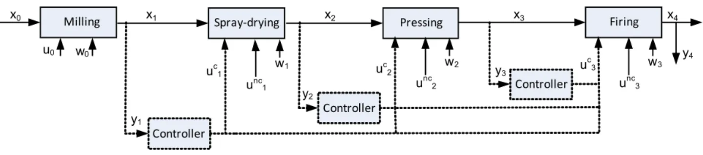
(15) variability.. 4.2. Feed-forward control process One of the main benefits of modelling a multi-stage manufacturing process is the ability to predict in advance the performance of downstream stages according to the performance of upstream stages. This prediction capability can lead engineers to fine-tune process parameters at downstream stages in order to maximise the final product quality. For instance, consider a manufacturing process of ceramic floor tiles where, after some measurements, it is known that the density of the slurry is slightly higher than it should be at the milling stage. With this information, the final spray-dried powder can be expected to present a slight higher percentage of moisture, which in turn will produce tiles with a lower apparent density after pressing and a higher dimensional contraction after firing. This problem could be minimised if, at the milling stage, this error propagation scheme is estimated by the use of the SoV model. In this case, the manipulated variables at spray drying, pressing and firing could be fine-tuned to compensate for the expected deviation of the tile dimension. This proposed control process scheme is called feed-forward control process, and it is described in Figure 2. x0. x1. Milling u0. x2. Spray-drying. w0 u. c 1. w1 unc1. uc2 y2. x3. Pressing w2 u. nc 2. u. y3. x4. Firing w3. c 3. Controller. u. y4. nc 3. Controller. y1 Controller. Figure 2. Feed-forward control scheme applied to the floor tile manufacturing process.. Under the feed-forward control strategy, the action that the controller should carry out can be derived from the SoV model as follows. Let us consider that at stage k, a measurement is conducted and thus yk is known. The variables to be controlled from previous stages, xk, can be estimated with yk given as:.

(16) By estimating the current variables, , the expected values of the variables to be controlled at the stage k+1 can be estimated in advance as:. At stage k+1, the manipulated variables uk+1 can be divided into two groups, those that can be easily modified (e.g. the flow rate of slurry at the spray dryer), and those that are preferably kept constant during production (e.g. the depression in the evaporation tower at the spray dryer). Denoting these manipulated variables as and , respectively, the previous equation is rewritten as:. where and are the corresponding matrices from that apply to and , respectively. In order to avoid any possible deviation from nominal values, the variables that can be modified at stage k+1, will be set up to ensure that the expectation of is 0, which means that the deviation due to upstream stages is being compensated by acting upon the current stage appropriately. Thus, the controller action is:. Therefore, applying this control strategy to all stages will ensure that the dimensional deviation of the tiles is minimum at the end of line.. 4.3. Monitoring and fault detection In order to detect out-of-control occurrences in multi-stage processes, one may monitor quality measurements of the product on the final stage using Statistical Process Control (SPC) techniques (Montgomery 2007), such as the Shewhart, the cumulative sum and the Exponentially Weighted Moving Average (EWMA) control charts for univariate quality measurement, and Hotelling’s T2 charts for multivariate cases. However, these univariate and multivariate tools are designed for a single-stage process, and cannot effectively identify an out-of-control stage in a multi-stage process (Xiang and Tsung 2008). Alternatively, one may also monitor quality measurements on individual stages by charting them separately. However, this approach ignores the fact that quality measurements on a certain stage are affected by the output quality from the preceding stages..

(17) For this reason, the application of variation propagation models in control charting has recently received great attention (Liu 2010). The variation propagation modelling capability provided by the engineering models (a model based on engineering knowledge that describes the physical relationships between controllable, manipulated and disturbance variables throughout the manufacturing process), especially the SoV models, significantly improves the SPC for multi-stage manufacturing processes. For instance, Xiang and Tsung (2008) designed a group EWMA (GEWMA) chart of One-Step ahead Forecast Error (OSFE) based on the Stream-of-Variation model and compared its performance with three alternative charts for multi-stage process monitoring: a group Shewhart charts of OSFE, individual EWMA charts and a Shewhart chart for the observations at the final stage. The study showed that the proposed chart was superior to the alternatives in detecting most shifts and, in comparison to group Shewhart charts, their approach was more sensitive to small and moderate shifts. In Zou and Tsung (2008) a directional multivariate GEWMA monitoring scheme was proposed where an engineering model was used to incorporate directional information about possible process shifts. Although the approach is similar to Zou and Tsung (2008), this a priori shift direction information is a particular characteristic in monitoring and diagnosing multi-stage processes and its used was proved to enhance the control chart performance. In this paper and for the sake of simplicity, we propose the approach presented in Xiang and Tsung (2008) for monitoring and detecting faulty stages based on the derived SoV model for the ceramic tile manufacturing process. To illustrate the procedure, let us rewrite the SoV model defined by Equations (1-2) in the form: (9) (10) where.

(18) since, for statistical monitoring, it is reasonable to assume that under in-control process the deviation of manipulated variables are normal distributed. Then, consider as the measurement vector observed from the jth sample on the kth stage in the process described by the SoV model in Equations (9-10). Given the measurement vectors from previous stages, , the standardized OSFE vector of , denoted as , can be defined with the following recursive formulations (see Xiang and Tsung 2008):. for . Based on the standardized OSFEs, for and , the multivariate EWMA statistic is constructed as. where is a smoothing constant satisfying . Note that is a vector where refers to the number of controllable variables at stage k. Then, Xiang and Tsung (2008) proposed the use of a GEWMA chart based on the statistic. where. and. Therefore, when exceeds the Upper Control Limit (UCL) of the chart, the GEWMA signals to indicate that the process is out of control. The faulty stage, denoted as , can be also identified by tracing the largest value of the GEWMA statistic as shows Equation (11) (11) The proposed approach for monitoring and fault detection in the multi-stage manufacturing process of ceramic floor tiles is illustrated in Figure 3 and a case study is shown in Section 5..

(19) x0. Milling. x1. Spray-drying. x2. y1 u0. w0. Pressing. y2 u1. x3. x4. Firing. y4. y3. w1. u2. u3. w2. w3. Statistical Process Control (SPC) based on SoV model Non-Fault Multivariate GEWMA control Chart. No. MZj > U.C.L.. Yes. 𝜁መ= 𝑎𝑟𝑔. max 𝑀𝑍𝑗. 1≤𝑘 ≤𝑁. Stage 𝜁መ Out of control. Figure 3. Monitoring and fault detection strategy by a GEWMA chart and the SoV model. 5. Case Study The proposed methodology is applied in a simplified floor tile manufacturing process which is based on experimental data reported in previous research works. The use of data from different research papers and, thus, different equipment, operators, raw materials and so on, let us validate the linearisation models required for the SoV model and, furthermore, let us define a SoV model structure that describes the ceramic floor manufacturing process in a generic form. This experimental data is presented in the Appendix and it is used to define the single-stage behaviour of the spray drier, the press and the kiln.. 5.1. Assumptions The SoV model derived in this case study is based on the following assumptions: -. At the milling stage, only the density of the slurry is considered as the controllable variable and the flow rate of water is considered as the manipulated variable. The flow rate of solids and deflocculant are considered to be constant. Thus, the equation that describes the system behaviour at this stage is , where is assumed to be ±0.08 g/cm3.. -. The errors in measuring the density of the slurry, moisture content of the spray-dried powder, bulk/apparent density and linear contraction are: s1 = ±0.05 g/cm3, s2 = ±0.05%, s3 = ±0.05 g/cm3 and s4 = ±0.05%, respectively, according to industrial practices.. 5.2. Resulting SoV model.

(20) The linearisation of the models, assuming normal conditions, is conducted around the following functioning points: . The matrices/vectors obtained from the linearisation are (see Appendix for details): . Stage 1: Milling. . Stage 2: Drying. . Stage 3: Pressing. . Stage 4: Firing. Following the proposed methodology, the resulting SoV model that explains the behaviour of this multi-stage manufacturing process in its input-output form is defined as:. where is a vector defined by ; and and are defined as ;. 5.3. Application of SoV model Given the SoV model defined above, the potential application of the model is studied in the following subsections.. 5.3.1. Detection of critical stages Firstly, the SoV model is applied to identify the critical stages or variables that have the greatest impact on the dimensional variability of the manufactured floor tiles. For this case study, it is assumed that, under normal operation, the manipulated variables present the inherent range of variability shown in Table 1, based on common industrial practices. Therefore, the percentage of.

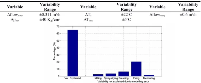
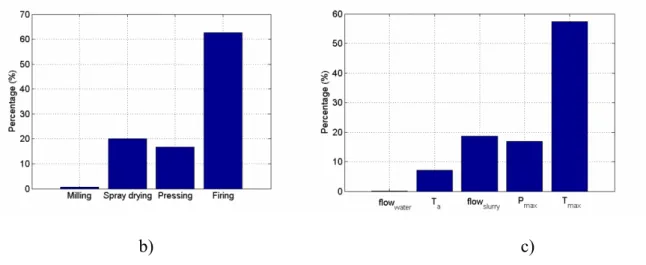
(21) variability explained by the SoV model and the modelling errors, the critical stages and process variables are identified by computing Equations (5-8). From Equation (5), the percentage of dimensional variability that is explained by the derived SoV model is 65% as it is shown in Figure 4a). Among the modelling errors (Equation (6)), the ones at the firing stage are the most relevant (20%) which means that the model at this stage could be improved. On the other hand, Equations (7-8) are computed to analyse critical stages and critical variables of the process. According to the results shown in Figure 4b) and 4c), the stage in which the ceramic tile is fired is the one that has the greatest influence on the final dimensional variability, accounting for 62% of the final variability of the floor tile. Therefore, it seems that an in-depth analysis of kiln performance should be conducted. The spray drying and pressing stages are also important for dimensional error propagation, with an impact of 20% and 16%, respectively. Milling does not seem to be important in this analysis (its influence is around 1% in the dimensional variability of the floor tiles), while the critical variables of the process are the maximum firing temperature, the flow rate of the slurry injected in the spray drying stage and the pressure in the pressing stage, in this order. Table 1. Variability of the parameters defined in U. Variable ∆flowwater ∆pmax. Variability Range ±0.311 m3/h ±40 Kg/cm2. Variability Range ±22ºC ±5ºC. Variable ∆Ta ∆Tmax. a). Variable ∆flowslurry. Variability Range ±0.6 m3/h.

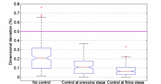
(22) b). c). Figure 4. a) Dimensional variability of ceramic tiles explained by the SoV model and the modelling errors at each stage; b) contribution to the total percentage of dimensional variability of ceramic tiles by each stage and c) by each process variable. 5.3.2. Feed-forward control process Secondly, the SoV model is applied to control the dimensional variability through implementing a feed-forward control scheme. To illustrate the capability of the controlling scheme, the final dimensional deviation of the tile is studied under three different approaches: i) without using a controller; ii) with a controller at the pressing stage; and iii) with a controller at the firing stage. The controller at the pressing stage modifies the maximum pressure to be exerted at the press according to the measurement of grain moisture previously conducted at the end of the spray drying stage and the expected apparent density of the tile estimated by the SoV model. Similarly, the controller at the firing stage modifies the maximum firing temperature of the kiln according to the measurement of the apparent density of the tile previously measured at the end of the pressing stage and the expected dimensional deviation of the tile estimated by the SoV model. Please, note that a controller at milling stage is not considered since the impact of this stage on dimensional quality is minor. These three approaches are compared by conducting 200 simulations using the process behaviour shown in Figure 5 which represents common production data from a tile industry in milling, spray drying, pressing and firing stages. For this case study, 0.5% dimensional deviation is the maximum deviation to classify the product as prime quality..

(23) Figure 6 shows the results of the final dimensional deviation of the floor tiles for each controlling strategy. The results show that the use of a feed-forward control approach improves the final quality of the floor tiles and prevents the production of calibers whereas the normal production generates 8.5% of parts as non-prime quality. The implementation of a controller at the pressing stage reduces the mean deviation of the tiles in 45% and the range of variation (six sigma range) in 44%; the controller at the firing stage reduces them in 67% and 65%, respectively. It is observed that the use of the feed-forward controller in the last stage (firing stage) outperforms the controller at the pressing stage due to the use of more information through the measurement at a later stage.. Figure 5. Process behaviour to evaluate the performance of different control strategies..

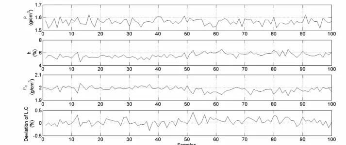
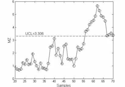
(24) Figure 6. Dimensional deviation of floor tiles under 3 different control approaches: i) without using a controller; ii) with a controller at the pressing stage; and iii) with a controller at the firing stage. 5.3.3. Monitoring and fault detection Finally, the SoV model is applied for monitoring and fault detection. For this purpose, it is assumed that the measurements are conducted at all stages, i.e, the slurry density at milling stage, the powder moisture at spray drying stage, the apparent density at pressing stage and dimensional deviation after the firing stage. The GEWMA chart previously discussed based on the proposed SoV model is used under the assumption that the process is in-control with the data shown in Table 1. As suggested in Xiang and Tsung (2008), the chart design parameters for a multi-stage manufacturing process with 4 stages and an ARL0 of 370 are set to and UCL = 3.306. To illustrate the effectiveness of the SoV model and its integration in a GEWMA control chart, 100 samples data are simulated. From sample 50 onwards, a shift in the resulting moisture content after the spray drying stage is added in order to simulate a faulty condition at this stage. The shift is 1.75 times the standard deviation from in-control. Figure 7 shows the measured values after each stage according to the simulated data and Figure 8 shows the values of the GEWMA control chart. As it can be seen, the chart detects the faulty condition after sample 57, and it points out that the faulty station is number 2, which refers to the spray drying stage..

(25) Figure 7. Values measured at each stage (simulated data). From top to bottom: slurry density (; moisture content of the spray-dried powder (h); the apparent density of the tile after pressing; and the deviation of the linear contraction after firing. At sample 50, a shift of size 1.75 times the standard deviation is added at the moisture content after spray drying.. Figure 8. GEWMA chart for monitoring the multi-stage manufacturing process of ceramic floor tiles. The chart detects the faulty process at sample 57, and identifies the stage 2 as the faulty stage which means the spray drying process. 6. Conclusions One of the main problems in the manufacture of floor tiles in the ceramic industry is the dimensional variability that may show up after firing the product, which leads to the product being classified in different calibers or dimensional qualities. Despite the extensive knowledge existing on the process of manufacturing ceramic floor tiles, few studies have sought to analyse the interactions among the different stages of the process in order to estimate the final dimensional variation of the product. In this paper a novel way of modelling the dimensional variability of ceramic floor tiles by the adaptation of the Stream of Variation (SoV) model has been proposed. The SoV model is obtained by using single-stage empirical models that are widely known in the literature, and which describe the relationships among the critical variables in each of the stages of the process. By integrating the single-stage models throughout the multi-stage process, the derived SoV model can.

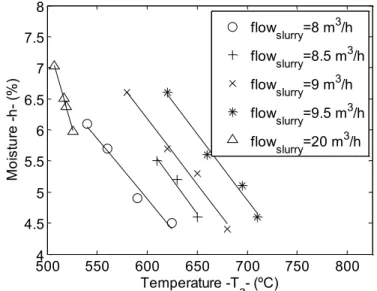
(26) be used in a large number of applications related to manufacturing improvement, such as detection of critical manufacturing stages, control and assurance of product quality through feed-forward control strategies, and monitoring and fast fault detection during production. A case study is presented to illustrate both the modelling methodology and its application. In this case study, the derived model is able to explain around 70% of dimensional variability of floor tiles and the application of the model by a feed-forward control scheme is able to reduce the dimensional variation up to 65%, preventing the production of calibers. The case study also demonstrates the use of the model for monitoring and fault detection which let manufacturers have a better understanding of the process increasing the dimensional control of ceramic floor tiles.. Acknowledgements This study was funded by the Generalitat Valenciana under the Research and Development Programme for Emerging Research Groups 2015, project GV/2015/091. The authors would like to thank Mr. Vicent Arnau and the floor tile manufacturing company Stylnul s.a. for their support and assistance with this project.. Appendix In order to define a generic SoV model for the ceramic floor tile manufacturing process, this Appendix gathers experimental data from different research works related to the operation of the spray dryer, the press and the kiln. Figure 9 (solid lines) shows the behaviour of the spray dryer reported in Negre et al. (1994) where it is observed the linearity of the moisture content of the resulting ceramic powder and the temperature of the air stream for a given slurry flow rate. Similar behaviour was identified in a local ceramic floor tile manufacturer as it is shown in Figure 9 (dashed line). Note that the different linear relationship is due to changes in the spray drier equipment, slurry formulation, number of spray nozzles, and flow rates of incoming and outgoing dry air. Therefore, the spray dryer can be defined by a generic linear equation in the form.

(27) In the case study presented in this paper, we assumed that the spray drier behaves according to the experimental data in Negre et al. (1994), thus, . 8 flowslurry=8 m3/h. 7.5. flowslurry=8.5 m3/h. Moisture -h- (%). 7. flowslurry=9 m3/h. 6.5. flowslurry=9.5 m3/h. 6. flowslurry=20 m3/h. 5.5 5 4.5 4 500. 550. 600 650 700 750 Temperature -Ta- (ºC). 800. Figure 9. Relationship of ceramic powder moisture and process variables at the spray drying stage. Solid lines refer to experimental data extracted from Negre et al. (1994); Dashed line refers to experimental data from a local floor tile manufacturer.. At the pressing stage, different studies have shown the impact of compaction pressure and moisture content of ceramic powder on the resulting apparent density after pressing. Figure 10 shows the data from four previous research works at different compaction pressures. All experimental data has a similar trend and a generic equation well accepted by practitioners is (Mallol et al. 2010, Amorós et al. 1983):. For the case study presented in this paper, we assume that the pressing stage behaves according to the experimental data in Amorós et al (1983) since this data is also presented in widely used technical manuals for manufacturing ceramic floor tiles (SACMI 2002). Thus, the coefficients are. ..

(28) compaction pressure (pmax) = 160 kg/cm2. 2400 2300. Heredia et al. (2011) Santos-Barbosa et al. (2013) Mallol et al. (2010) Amoros et al. (1983). 2400 2300. a. 2200. Apparent Density -. Apparent Density -. 2500. - (kg/m3). Heredia et al. (2011) Santos-Barbosa et al. (2013) Mallol et al. (2010) Amoros et al. (1983). a. - (kg/m3). 2500. compaction pressure (pmax) = 270 kg/cm2. 2100 2000 1900 1800 1700 4. 4.5. 5 5.5 Moisture -h- (%). 6. 6.5. 2200 2100 2000 1900 1800 1700 4. 4.5. 5 5.5 Moisture -h- (%). 6. 6.5. Figure 10. Relationship of the apparent density and process variables at the pressing stage reported in different research works.. Finally, the kiln operation determines the vitrification of the composition of the floor tile and, thus, the linear contraction and the final dimensions. Figure 11 shows the experimental data reported in different research works where a relationship between apparent density, firing temperature and linear contraction can be found. Note that the differences are mainly due to the different composition of the floor tiles at each research, which produces different vitrification diagrams. Since the firing temperature is usually set up within a small range, a generic linear equation can be defined in the form. In the case study presented in this paper, we assumed that, for a given tile composition, the firing stage behaves according to the experimental data in SACMI (2002), thus, . apparent density ( a) = 2.02 g/cm3. apparent density ( a) = 1.93 g/cm3. 10 9. Santos-Barbosa et al. (2013) Escardino et al. (1981) Amoros et al. (1983) SACMI (2002). 8 7 6 5 4 3 1050. 1100 1150 1200 Firing Temperature -Tmax- (ºC). 11. Linear Contraction -L.C- (%). Linear Contraction -L.C- (%). 11. 10 9. Santos-Barbosa et al. (2013) Escardino et al. (1981) Amoros et al. (1983) SACMI (2002). 8 7 6 5 4 3 1050. 1100 1150 1200 Firing Temperature -Tmax- (ºC).

(29) Figure 11. Relationship of the linear contraction of tiles at firing stage reported in different research works. 8.. References. Abellan-Nebot, J.V., Liu, J., Romero, F. (2012a). Quality prediction and compensation in multistation machining processes using sensor-based fixtures. Robotics and Computer-Integrated Manufacturing 28 (2): 208–19. doi:10.1016/j.rcim.2011.09.001. Abellan-Nebot, J.V, Liu, J., Romero, F. (2012b). State space modeling of variation propagation in multistation machining processes considering machining-induced variations. Journal of Manufacturing Science and Engineering 134 (2): 21002. doi:10.1115/1.4005790. Abellan-Nebot, J. V., Liu, J., Romero, F. (2012c). Stream-of-variation based quality assurance for multi-station machining processes - Modeling and Planning. In Statistical and Computational Techniques in Manufacturing, edited by J. Paulo Davim, 55-99, Springer Berlin Heidelberg. Abellan-Nebot, J.V., Liu, J., Romero, F. (2013). Process-oriented tolerancing using the extended stream. of. variation. model.. Computers. in. Industry. 64. (5):. 485–98.. doi:10.1016/j.compind.2013.02.005. Amorós, J. L., Beltrán, V., Negre, F., Escardino, A. (1983). Estudio de la compactación de soportes cerámicos (bizcochos) de pavimento y revestimiento-II: influencia de la presión y humedad de prensado. Boletín de la Sociedad Española de Cerámica y Vidrio 22: 9–18. Andreola, F., Siligardi, C., Manfredini, T., Carbonchi, C. (2009). Rheological behaviour and mechanical properties of porcelain stoneware bodies containing italian clay added with bentonites. Ceramics International 35 (3): 1159–64. doi:10.1016/j.ceramint.2008.05.017. Barrachina, E., Llop, J., Notari, M.D., Fraga, D., Martí, R., Calvet, I., Carda, J.B. (2015). Rheological effect of different deflocculation mechanisms on a porcelain ceramic composition. Journal of Chemical Technology & Metallurgy, 50(4): 493-502. Blasco, A., Enrique, J.E., Arrebola, C. (1982). Los defloculantes y su acción en las pastas cerámicas para atomización.” I Congreso Iberoamericano de Cerámica, Vidrio y Refractarios. Tomo II: 265–75. Bonavia, T., Marin, J.A. (2006). An empirical study of lean production in the ceramic tile industry in Spain. International Journal of Operations & Production Management 26 (5): 505–31. doi:10.1108/01443570610659883. Chen, Y., Ding, Y., Jin, J., Ceglarek, D. (2006). Integration of process-oriented tolerancing and.

(30) maintenance planning in design of multistation manufacturing processes. IEEE Transactions on Automation Science and Engineering 3 (4): 440–53. doi:10.1109/TASE.2006.872105. Da Silva, J.G.B., de Carvalho, E.F.U., Kuhnen, N.C., Riella, H.G., Bernardin, A.M. (2008). Influence of processing water on ceramic suspension viscosity. In Proceedings of World Congress on Ceramic Tile Quality, Castellon, Spain, 119–124. De Noni, A., de Oliveira Modesto, C., Hotza, D. (2006). Mathematical modelling applied to the dimensional control of ceramic tiles produced by the single firing and wet milling route. In Proceedings of World Congress on Ceramic Tile Quality, Castellon, Spain, pp. 227–32. Ding, Y., Ceglarek, D., Shi, J. (2002). Fault diagnosis of multistage manufacturing processes by using state space approach. Journal of Manufacturing Science and Engineering – Transactions of the ASME 124 (2): 313–22. doi:10.1115/1.1445155. Ding, Y., Pansoo, K., Ceglarek, D., Jin, J. (2003). Optimal sensor distribution for variation diagnosis in multistation assembly processes. IEEE Transactions on Robotics and Automation 19 (4): 543–56. Escardino, A., Amorós, J.L., Enrique, J.E. (1981). Estudio de pastas de gres para pavimentos. Boletín. de. la. Sociedad. Española. de. Cerámica. y. Vidrio. 20. (1):. 17–24.. doi:13.1017/CBO9781107415324.004. Ferrer, C., Llorens, D., Mallol, G., Monfort, E., Moreno, A. (1994). Optimización de las condiciones de funcionamiento en hornos monoestrato. Medida de gradientes transversales de temperatura. Técnica Cerámica 227: 653–62. Galos, K. (2011). Influence of mineralogical composition of applied ball clays on properties of porcelain tiles. Ceramics International, 37(3): 851-861. doi:/10.1016/j.ceramint.2010.10.014 Heredia, J.A., Gras, M. (2010). Empirical procedure for modeling the variation transmission in a manufacturing. process.. Quality. Engineering. 22. (3):. 150–56.. doi:10.1080/08982111003724929. Heredia, J.A., Gras, M. (2011). Statistical estimation of variation transmission model in a manufacturing process. International Journal of Advanced Manufacturing Technology 52 (5–8): 789–95. doi:10.1007/s00170-010-2735-y. Jabnoun, N. (2002). Control processes for total quality management and quality assurance. Work Study, 51(4): 182-190. doi:10.1108/00438020210430733 Jarque, J.C., Cantavella, V., Daroca, M.J., Gómez, P., Arrébola, C., Carceller, A. (2002). Influencia de las condiciones de operación del horno de rodillos sobre la curvatura de las piezas. In.

(31) Proceedings of World Congress on Ceramic Tile Quality, Castellon, Spain, 149–52. Jin, Jionghua, and Jianjun Shi. 1999. “State Space Modeling of Sheet Metal Assembly for Dimensional Control.” Journal of Manufacturing Science and Engineering 121 (4): 756–62. doi:10.1115/1.2833137. Liu, J. (2010). Variation reduction for multistage manufacturing processes: a comparison survey of Statistical-Process-Control vs Stream-of-Variation methodologies. Quality and Reliability Engineering International, 26(7): 645-661. doi: 10.1002/qre.1148 Loose, J.P., Zhou, Q., Zhou, S., Ceglarek, D. (2010). Integrating GD&T into dimensional variation models for multistage machining processes. International Journal of Production Research 48 (11): 3129–49. doi:10.1080/00207540802691366. Mallol, G., Llorens, D., Boix, J., Pascual, N., Poyatos, A., Bonaque, R. (2012). Measurement and control of maximum pressure in the cavities of a die for ceramic tile manufacture. In Proceedings of World Congress on Ceramic Tile Quality, Castellon, Spain, 1–15. Mondragon, R., Jarque, J.C:, Julia, J.E., Hernandez, L., Barba, A. (2012). Effect of slurry properties and operational conditions on the structure and properties of porcelain tile granules dried in an acoustic. levitator.. Journal. of. the. European. Ceramic. Society. 32. (1).. 59–70.. doi:10.1016/j.jeurceramsoc.2011.07.025. Montgomery, D. C. (2007). Introduction to statistical quality control. John Wiley & Sons, ISBN 978-0470169926. Negre, F., Jarque, J.C., Fetiu, C., Enrique, J.E. (1994). Study of the spray-drying operation of ceramic powders on an industrial scale, its control and automation. Evolution, 105–16. Negre, F., Sánchez, E. (1996). Advances in spray-dried pressing powder processes. Science of Whitewares, 169–81. Poyatos, A., Bonaque, R., Mallol, G., Boix, J. (2010). Nuevo sistema y metodología para la eliminación de los calibres en el proceso de fabricación de baldosas cerámicas. Boletin de la Sociedad Espanola de Ceramica y Vidrio, 49(2): 147–152. SACMI, (2002), Applied Ceramic Technology, Editrice La Mandragora of Imola s.r.l., ISBN 8888108-48-3 Santos-Barbosa, D., Hotza, D., Boix, J., Mallol, G. (2013). Modelling the influence of manufacturing process variables on dimensional changes of porcelain tiles. Advances in Materials Science and Engineering. doi:10.1155/2013/142343. Xiang, L., Tsung, F. (2008). Statistical monitoring of multi-stage processes based on engineering.

(32) models. IIE transactions, 40(10): 957-970. doi: 10.1080/07408170701880845 Zhou, S., Huang, Q., Shi, J. (2003). State space modeling of dimensional variation propagation in multistage machining process using differential motion vectors. IEEE Transactions on Robotics and Automation 19 (2): 296–309. doi:10.1109/TRA.2003.808852. Zou, C., Tsung, F. (2008). Directional MEWMA schemes for multistage process monitoring and diagnosis. Journal of Quality Technology, 40(4): 407..

(33)

(34)