Building Data Warehouses with Semantic Web Data

Texto completo

(1)Building Data Warehouses with Semantic Web Data Victoria Nebot∗, Rafael Berlanga Departamento de Lenguajes y Sistemas Informáticos Universitat Jaume I Campus de Riu Sec, 12071, Castellón, Spain Phone: (+34) 964 72 83 67. Fax: (+34) 964 72 84 35. Abstract The Semantic Web (SW) deployment is now a realization and the amount of semantic annotations is ever increasing thanks to several initiatives that promote a change in the current Web towards the Web of Data, where the semantics of data become explicit through data representation formats and standards such as RDF/(S) and OWL. However, such initiatives have not yet been accompanied by efficient intelligent applications that can exploit the implicit semantics and thus, provide more insightful analysis. In this paper, we provide the means for efficiently analyzing and exploring large amounts of semantic data by combining the inference power from the annotation semantics with the analysis capabilities provided by OLAP-style aggregations, navigation, and reporting. We formally present how semantic data should be organized in a well-defined conceptual MD schema, so that sophisticated queries can be expressed and evaluated. Our proposal has been evaluated over a real biomedical scenario, which demonstrates the scalability and applicability of the proposed approach. Keywords: Semantic Web, Ontologies, Data Warehouses, OLAP, Multidimensional design. 1. Introduction The effort behind the Semantic Web (SW) is to add machine-understandable, semantic annotation to web-published contents so that web information can be effectively retrieved and processed by both humans and machines in a great variety of tasks. This is in practice achieved by using SW technologies, which enable to attach semantics to resources, ranging from very simple to very complex annotations depending on the requirements. SW technologies open a new dimension to data integration by providing a common terminology, standard for∗ Corresponding. author Email addresses: romerom@lsi.uji.es (Victoria Nebot), berlanga@lsi.uji.es (Rafael Berlanga). Preprint submitted to Elsevier. May 27, 2011.

(2) mats for knowledge resources (e.g., RDF/(S)1 and OWL2 ), semantically linked data, and more formal representations like description logic axioms for inference tasks. As a result, more and more semi-structured data and knowledge resources are being published in the Web, creating what is called the Web of Data [11]. At the same time, there is a great urgency of new analytical tools able to summarize and exploit all these resources. Semantic search has emerged as one of the first applications making use and exploiting the Web of Data. New systems that offer search and browsing over RDF data have been developed [20, 19, 39, 16, 40]. Research in this area is a hot topic because it enhances conventional information retrieval by providing search services centered on entities, relations, and knowledge. Also, the development of the SW demands enhanced search paradigms in order to facilitate acquisition, processing, storage, and retrieval of semantic data. Albeit interesting, semantic search does not provide users with great insight into the data. Various advanced applications that have recently emerged impose modern user and business needs that require a more analytical view. Some examples include customer support, product and market research or life sciences and health care applications with both structured and unstructured information available. The biomedical domain is one of the most active areas where significant efforts have been spent to export database semantics to data representation formats following open standards, which explicitly state the semantics of the content. The use of ontologies and languages such as RDF and OWL in the area of medical sciences has already a long way, and several web references to medical ontologies for different areas of medicine can be found (UMLS [12], SNOMED-CT [6], GALEN [1], GO [2], etc.) Moreover, a growing penetration of these technologies into the life science community is becoming evident through many initiatives (e.g. Bio2RDF [9], Linked Life Data [3], Liking Open Drug Data [4], etc.) and an increasing number of biological data providers, such as UniProt [7], have started to make their data available in the form of triples. In these complex scenarios keyword or faceted search may be useful but not enough, since advanced analysis and understanding of the information stored are required. Given the previous analysis requirements over these new complex and semantic representation formats, the well-known data warehousing (DW) and OLAP technologies seem good candidates to perform more insightful analytical tasks. During the last decade, DW has proved its usefulness in traditional business analysis and decision making processes. A data warehouse can be described as a decision-support tool that collects its data from operational databases and various external sources, transforms them into information and makes that information available to decision makers in a consolidated and consistent manner [24]. One of the technologies usually associated to DW is multidimensional (MD) processing, also called OLAP [17] processing. MD models define the an1 RDF/(S): 2 OWL:. http://www.w3.org/TR/rdf-concepts/ , rdf-schema/, ’04 http://www.w3.org/TR/owl-features/, ’04.. 2.

(3) alytic requirements for an application. It consists of the events of interest for an analyst (i.e., facts) described by a set of measures along with the different perspectives of analysis (dimensions). Every fact is described by a set of dimensions, which are organized into hierarchies, allowing the user to aggregate data at different levels of detail. MD modeling has gained widespread acceptance for analysis purposes due to its simplicity and effectiveness. This work opens new interesting research opportunities for providing more comprehensive data analysis and discovery over semantic data. In this paper, we concentrate on semantic annotations that refer to an explicit conceptualization of entities in the respective domain. These relate the syntactic tokens to background knowledge represented in a model with formal semantics (i.e. an ontology). When we use the term “semantic”, we thus have in mind a formal logical model to represent knowledge. We provide the means for efficiently analyzing and exploring large amounts of semantic data by combining the inference power from the annotation semantics with the analysis capabilities provided by OLAP-style aggregations, navigation, and reporting. We formally present how semantic data should be organized in a well-defined conceptual MD schema, so that sophisticated queries can be expressed and evaluated. As far as we know there is no tool providing OLAP-like functionality over semantic web data. In Section 2.3 we elaborate on the requirements and challenges faced when dealing with semantic web data. The main contributions of the paper are summarized as follows: • We introduce a semi-automatic method to dynamically build MD fact tables from semantic data guided by the user requirements. • We propose two novel algorithms to dynamically create dimension hierarchies with “good” OLAP properties from the taxonomic relations of domain ontologies for the fact tables generated with the previous method. • We provide an application scenario and a running use case in the biomedical domain to illustrate the usefulness and applicability of our method. The rest of the paper is organized as follows. Section 2 introduces the application scenario with a use case that motivates our approach. Section 3 provides an overview of the method. Section 4 contains the user conceptual MD schema definition. Section 5 is devoted to the Fact Extraction process, and we cover both the foundations and implementation issues. In Section 6, we propose two methods for Dimension Extraction. Section 7 describes the experimental evaluation and implementation. Section 8 reviews related work regarding the trends in analytical tools for non-conventional data sources, mainly the semi-structured ones and finally, in Section 9 we give some conclusions and future work. 2. Application scenario In this paper we adopt the application scenario of the Health-e-Child integrated project (HeC) [37], which aimed to provide a grid-based integrated data 3.

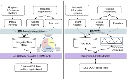
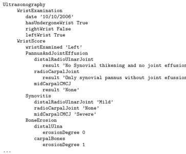
(4) Hospitals Information Systems. Patient Records. Hospitals Information Systems. Hospitals Departments. Clinical Reports. Hospitals Departments. Patient Records. Raw data. XML-based representation. Clinical Reports. Raw data. RDF/OWL. Integrated Data Model. Triple Store Reference Ontologies. HeC Gateway (includes a DBMS API). Dimension & Fact Extractor. Clinician DSS Tools (ad hoc applications). DSS OLAP-based tools. Figure 1: HeC data integration architecture (left hand) versus the Semantic Web integration architecture (right hand). infrastructure for new decision support systems (DSS) for Paediatrics. Such DSS tools are mainly focused on traditional diagnosis/prognosis tasks and patient follow-up. This scenario regards three main types of data sources: well standardized records coming from hospital information systems (e.g. HL7-conformant records), highly heterogeneous semi-structured clinical reports, and a variety of unstructured data such as DICOM files, ECG data, X-ray and ultrasonography images. All data are delivered to the HeC infrastructure in XML format, usually lacking of any schema for the semi- and unstructured data sources. Unfortunately, most of the interesting analysis dimensions are located in the schema-less data sources. The integration solution proposed in the HeC project formerly consisted of defining a flexible integrated data model [10], which is built on top of a grid-aware relational database management system (see left hand side of Figure 1). As clinical reports present very irregular structures (see the example presented in Figure 2), they are decomposed and classified into a few organizational units (i.e. patient, visit, medical event and clinical variables), thus disregarding much information that could be useful for the intended DSS tools. Additionally, this data model also includes tables that map clinical variables to concept identifiers from the UMLS Metathesaurus [12]. These tables are intended to link patient data to bibliographic resources such as MEDLINE [5]. It is worth mentioning that a similar scenario and solution have been proposed in. 4.

(5) the OpenEHR initiative3 . However, in this paper we adopt a different integration architecture (see right hand side of Figure 1), which follows the current trends in biomedical [13] and bioinformatics data integration [27], and relies entirely on SW technology. In this architecture, the integrated data model is defined as an application ontology that models the health care scenario (e.g. patients, visits, reports, etc.) This ontology can import concepts defined in external knowledge resources (reference domain ontologies in Figure 1). Finally, the biomedical data is semantically annotated according to the application ontology and stored as RDF triples (i.e. triple store). In the HeC scenario, the application ontology modeling the rheumatology domain has 33 concepts and 39 roles. However, this ontology can import any concept from UMLS, which is used as reference domain ontology, and contains over 1.5 million concepts. The triple store of the application scenario has 605420 instances containing references to 874 different concepts of UMLS. Moreover, depending on the user’s requirements (i.e. dimensions selected) more domain ontology axioms will be imported in order to build the dimension hierarchies. In this paper, we aim at analyzing and exploiting all this semantic data through OLAP-based tools. Subsequent sections present the representation formalism of the semantic data, some examples of OLAP-based analysis, and finally, the main issues involved in carrying out OLAP-based analysis over semantic data. 2.1. Semantic Data Representation We use the language OWL-DL to represent the application ontology to which semantic annotations refer. OWL-DL has its foundation in the description logics (DL) [8]. Basically, DLs allow users to define the domain of interest in terms of concepts (called classes in OWL), roles (called properties in OWL) and individuals (called instances in OWL). Concepts can be defined in terms of other concepts and/or properties by using a series of constructors, namely: concept union (t), intersection (u) and complement (¬), as well as enumerations (called oneOf in OWL) and existential (∃), universal (∀) and cardinality (≥, ≤, =) restrictions over a role R or its inverse R− . Concept definitions are asserted as axioms, which can be of two types: concept subsumption (C v D) and concept equivalence (C ≡ D). The former one is used when one only partially knows the semantics of a concept (the necessary but not sufficient conditions). Equivalence and subsumption can be also asserted between roles, and roles can have special constraints (e.g., transitivity, symmetry, functionality, etc.) The set of asserted axioms over concepts and roles is called the terminological box (T Box). Semantic data is expressed in terms of individual assertions, which can be basically of two types: assert the concept C of an individual a, denoted C(a), 3 http://www.openehr.org/home.html. 5.

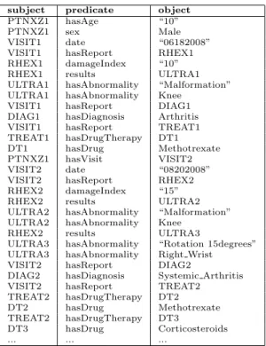
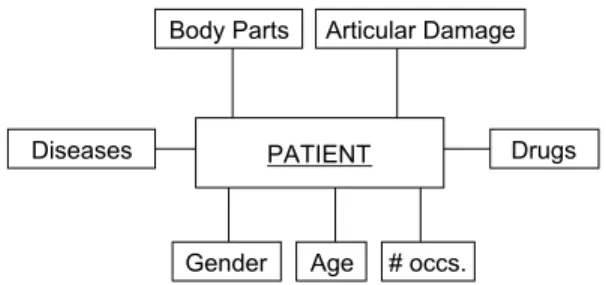
(6) Ultrasonography WristExamination date ’10/10/2006’ hasUndergoneWrist True rightWrist False leftWrist True WristScore wristExamined ’Left’ PannusAndJointEffusion distalRadioUlnarJoint result ’No Synovial thikening and no joint effusion’ radioCarpalJoint result ’Only synovial pannus without joint efussion midCarpalCMCJ result ’None’ Synovitis distalRadioUlnarJoint ’Mild’ radioCarpalJoint ’None’ midCarpalCMCJ ’Severe’ BoneErosion distalUlna erosionDegree 0 carpalBones erosionDegree 1 .... Figure 2: Fragment of a clinical report of the Rheumatology domain.. and assert a relation between two individuals a and b, denoted R(a, b). The set of assertions over individuals is called the assertional box (ABox). For practical purposes, the T Box and the ABox are treated separately. Notice that while the ABox is usually very dynamic for it is constantly updated, the T Box hardly changes over time. From now on, we will use the term ontology to refer to the T Box, and instance store to refer to the ABox storage system. We assume that the instance store is always consistent w.r.t. the associated ontology. Figure 3 shows a fragment of the ontology designed for patients with rheumatic diseases in our application scenario, whereas Table 1 shows a fragment of an instance store associated to this ontology. In this case, the instance store is expressed as triples (subject, predicate, object), where a triple of the form (a, type, C) corresponds to a DL assertion C(a), and otherwise the triple (a, R, b) represents the relational assertion R(a, b). 2.2. Example of Use Case In the previous application scenario, we propose as use case to analyze the efficacy of different drugs in the treatment of inflammatory diseases, mainly rheumatic ones. At this stage, the analyst of this use case should express her analysis requirements at a conceptual level. Later on, these requirements will be translated into dimensions and measures of a MD schema that will hold semantic data. Figure 4 depicts the conceptual model of the analyst requirements where the central subject of analysis is Patient. The analyst is interested in exploring the patient’s follow-up visits according to different parameters such as gender, 6.

(7) P atient v = 1 hasAge.string P atient v = 1 sex.Gender P atient v ∀ hasGeneReport.GeneP rof ile GeneP rof ile v ∀ over.Gene u ∀ under.Gene P atient v ∀ hasHistory.P atientHistory P atientHistory v ∃f amilyM ember.F amily Group u ∃ hasDiagnosis.Disease or Syndrome P atient v ∃ hasV isit.V isit V isit v = 1 date.string V isit v ∀ hasReport.(Rheumatology t Diagnosis t T reatment t Laboratory) Rheumatology v ∃ results.(Articular t ExtraArticular t U ltrasonography) Rheumatology v = 1 damageIndex.string U ltrasonography v ∀ hasAbnormality.Disease or Syndrome U ltrasonography v ∀ location.Body Space or Junction ArticularF inding v ∃ af f ectedJoint.Body Space or Junction ArticularF inding v ∀ examObservation.string Diagnosis v ∃ hasDiagnosis.Disease or Syndrome T reatment v = 1 duration.string T reatment v ∃ hasT herapy.DrugT herapy DrugT herapy v = 1 administration.AD DrugT herapy v = 1 hasDrug.P harmacologic Substance AD v ∃ dosage.string u ∃ route.string u ∃ timing.string Laboratory v ∃ bloodIndicants.( ∃ cell.Cell u ∃ result.string u ∃ test.Lab P rocedure) Rheumatoid Arthritis v Autoimmune Disease Autoimmune Disease v Disease or Syndrome .... Figure 3: Ontology axioms (Tbox).. 7.

(8) subject PTNXZ1 PTNXZ1 VISIT1 VISIT1 RHEX1 RHEX1 ULTRA1 ULTRA1 VISIT1 DIAG1 VISIT1 TREAT1 DT1 PTNXZ1 VISIT2 VISIT2 RHEX2 RHEX2 ULTRA2 ULTRA2 RHEX2 ULTRA3 ULTRA3 VISIT2 DIAG2 VISIT2 TREAT2 DT2 TREAT2 DT3 .... predicate hasAge sex date hasReport damageIndex results hasAbnormality hasAbnormality hasReport hasDiagnosis hasReport hasDrugTherapy hasDrug hasVisit date hasReport damageIndex results hasAbnormality hasAbnormality results hasAbnormality hasAbnormality hasReport hasDiagnosis hasReport hasDrugTherapy hasDrug hasDrugTherapy hasDrug .... object “10” Male “06182008” RHEX1 “10” ULTRA1 “Malformation” Knee DIAG1 Arthritis TREAT1 DT1 Methotrexate VISIT2 “08202008” RHEX2 “15” ULTRA2 “Malformation” Knee ULTRA3 “Rotation 15degrees” Right Wrist DIAG2 Systemic Arthritis TREAT2 DT2 Methotrexate DT3 Corticosteroids .... Table 1: Semantic annotations (Abox).. 8.

(9) age, the drugs prescribed, the affected body parts, the diseases diagnosed, the articular damage and the number of occurrences. Body Parts. Diseases. Articular Damage. Drugs. PATIENT. Gender. Age. # occs.. Figure 4: Use case analysis requirements.. Later on, the previous analysis requirements will be formally expressed in terms of DL expressions over the ontology and these expressions will be mapped to elements of a MD schema (i.e. dimensions and measures) that will eventually be populated with the semantic annotations of the instance store. The ultimate goal of the approach is to effectively analyze and explore the semantic annotations using OLAP-style capabilities. In this use case, the analyst will be able to specify useful MD queries in order to analyze patient data and discover useful patterns and trends. As an example, we show two MD queries expressed in MDX-like syntax that an analyst would execute over the resulting fact table in order to generate cubes. The first query builds a cube where for each administered drug and diagnosed disease the articular damage registered is averaged. By exploring this cube the analyst can find out interesting patterns such as which drugs mitigate the articular damage depending on the disease type. CREATE CUBE [cubeArticularDamage1] FROM [patient_dw] ( MEASURE [patient_dw].[avgArtDamIndex], DIMENSION [patient_dw].[Drug], DIMENSION [patient_dw].[Disease] ). The second query builds a cube where the articular damage is explored over different analysis perspectives, namely the affected body parts and the patient’s gender. This way the analyst can discover which body parts contribute most to the total damage index contrasted by gender. CREATE CUBE [cubeArticularDamage2] FROM [patient_dw] ( MEASURE [patient_dw].[avgArtDamIndex], DIMENSION [patient_dw].[BodyPart], DIMENSION [patient_dw].[Gender] ). 9.

(10) 2.3. Issues in analyzing semantic data The full exploitation of semantic data by OLAP tools is far from trivial due to the special features of semantic data and the requirements imposed by OLAP tools. Next, we describe some of the main challenges we encounter when dealing with semantic web data, which are treated in this paper: • Usability: When dealing with the Web of Data, the user typically needs to specify a structured query in a formal language like SPARQL. However, the end user often does not know the query language and the underlying data graph structure. Even if she did, languages such as SPARQL do not account for the complexity and structural heterogeneity often common in RDF data. We overcome this issue by providing the user with a simple mechanism to specify her analysis requirements at the conceptual level. We ask the user to compose a conceptual MD schema by selecting concepts and properties of interest from the available ontologies. • Imprecision: The information needs expressed by the user might be imprecise. On one hand, the flexibility and ease of use offered to the user in the requirements phase can lead to an ambiguous specification (i.e. the concepts and properties selected might be used in several contexts in the ontologies). On the other hand, the user might have limited knowledge about the domain and her specification might be too general or abstract. Our method overcomes both types of imprecision by taking into account all possible interpretations of the concepts specified by the user. Moreover, thanks to the semantics attached to the data, implicit information can be derived and made explicit so that the user can refine her MD specification by selecting these new inferred concepts. • Scalability: As the amount of available data is ever growing, the ability to scale becomes essential. What is more important, scalability is known to be an issue when reasoning with large ontologies. In this work, we overcome this issue by applying specific indexes to ontologies in order to handle basic entailments minimizing the use of the reasoner. • Dynamicity: The web is continuously changing and growing. Therefore, analytical tools should reflect these changes and present fresh results. Also, data are being provided at an overwhelming level of detail and only a subset of attributes constitute meaningful dimensions and facts for the analyst. For these reasons, our method allows the user to select only the concepts of interest for analysis and automatically derives a MD schema (i.e. dimensions and facts) and its instantiation ready to be fed into an off the shelf OLAP tool, for further analysis. 3. Method overview In this section we present an overview of our method. We focus on the endto-end description of the data flow from expressing the analysis requirements 10.

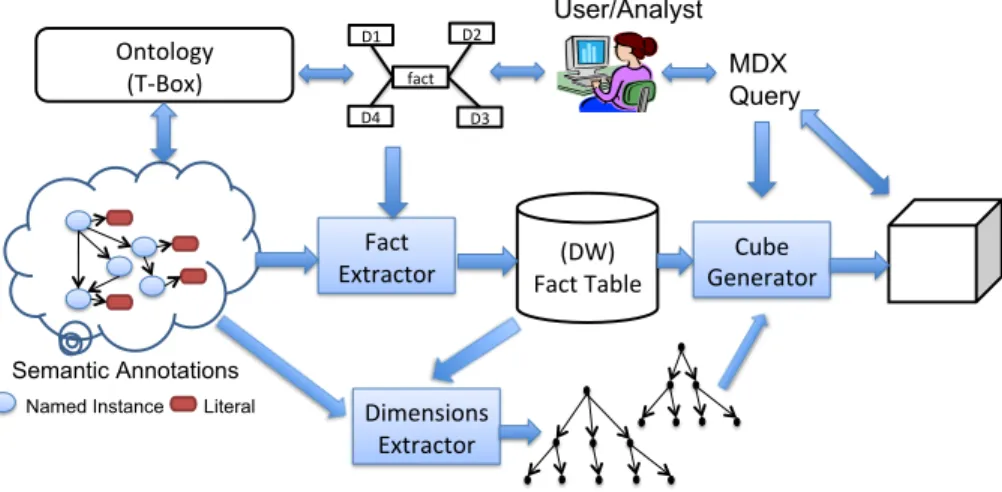
(11) to returning analytical query results. Figure 5 depicts a schematic overview of the whole process. The repository of semantic annotations on the left of Figure 5 stores both the application and domain ontology axioms (i.e. Tbox ) and the semantic annotations (i.e. instance store). This repository maintains the necessary indexes for an efficient management. For obtaining OLAP style functionality, our goal is to create a MD schema from both the analyst requirements and the knowledge encoded in the ontologies. The fact table is populated with facts extracted from the semantic annotations –a fact is not a simple RDF triple but a valid semantic combination of structurally related instances– while dimension hierarchies are extracted by using the subsumption relationships inferred from the domain ontologies. Each of the phases are described in turn.. Ontology (T‐Box). D2. D1. User/Analyst MDX Query. fact D4. D3. Fact Extractor. (DW) Fact Table. Cube Generator. Semantic Annotations Named Instance. Literal. Dimensions Extractor. Figure 5: Architecture for semantic annotations analysis.. • During the design of the conceptual MD schema, the user expresses her analysis requirements in terms of DL expressions over the ontology. In particular, she selects the subject of analysis, the potential semantic types for the dimensions and the measures. • The fact extractor is able to identify and extract facts (i.e. valid combinations of instances) from the instance store according to the conceptual MD schema previously designed, giving rise to the base fact table of the DW. • The dimensions extractor is in charge of building the dimension hierarchies based on the instance values of the fact table and the knowledge available in the domain ontologies (i.e. inferred taxonomic relationships) while also considering desirable OLAP properties for the hierarchies. • Finally, the user can specify MD queries over the DW in order to analyze and explore the semantic repository. The MD query is executed and a 11.

(12) cube is built. Then, typical OLAP operations (e.g., roll-up, drill-down, dice, slice, etc.) can be applied over the cube to aggregate and navigate data. 4. Multidimensional schema definition In this section, we present how the analyst information requirements are translated into a conceptual MD schema in order to leverage the aggregation power of OLAP. The analyst defines the MD elements with DL expressions, which seems the most natural choice given that the data sources are expressed under this logical formalism. In particular, the MD schema contains the following elements: • Subject of analysis: the user selects the subject of analysis from the ontology concepts. We name this concept CSU B . • Dimensions: usually, a dimension is defined as a set of levels with a partial order relation among them (i.e., hierarchy). We postpone the hierarchy creation of each dimension in order to dynamically adapt it to the base dimension values appearing in the resulting fact table. Therefore, the analyst must specify just the semantic type of each dimension. They can be either concepts, named C, or data type properties, named dtp, selected from the ontology. • Measures: The user selects measures from the ontology by specifying the numeric data type property dtp and the aggregation function to be applied (i.e., sum, average, count, min, max, etc). Notice that at this point, the analyst does neither know the dimension values nor the roll-up relationships that will eventually be used in the resulting MD schema. The method presented in this paper will automatically capture this information from the application and the domain ontologies involved in the analysis but always taking into account the user requirements. The syntax for the definition of the MD elements is specified in Figure 6 by means of a version of Extended BNF where terminals are quoted and non-terminals are bold and not quoted. For the running use case, the MD schema definition is shown in Figure 7. 5. Extracting Facts This section addresses the process of fact extraction from the semantic annotations. First, the foundations of the approach are presented and then we discuss implementation details.. 12.

(13) 0. 0. subject ::= SU BJECT ( name 0. 0. dimension ::= DIM ( name 0. 0. measure ::= M ( name. 0 0. 0 0. , concept ). 0 0. 0 0. , concept | datatypeprop ). 0 0. 0 0. 0. , numValueFunction ( datatypeprop )). name ::= identifier concept ::= concept definition according to OWL DL syntax datatypeprop ::= datavaluedPropertyID 0. 0. 0. 0. 0. 0. 0. 0. 0. numValueFunction ::= AV G | SU M | COU N T | M AX | M IN datavaluedPropertyID ::= URIreference identifier ::= valid string identifier. Figure 6: BNF syntax for MD schema specification. SU BJECT ( P atientCase , P atient ) DIM ( Disease , Disease or Syndrome) DIM ( Drug , P harmacological Substance) DIM ( Age , hasAge) DIM ( Gender , Gender) DIM ( BodyP art , Body Space Or Junction) M ( AvgArtDamIndex , AV G (damageIndex) M ( N umberOccs. , COU N T (P atientCase)). Figure 7: MD schema specification for the use case. 13. 0. 0.

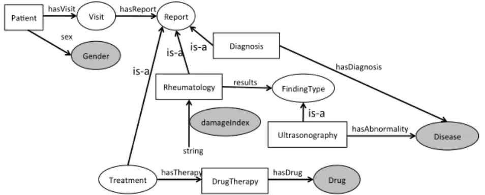
(14) 5.1. Foundations The ultimate goal of the approach is to identify and extract valid facts according to the user’s requirements. However, the user’s conceptual MD schema is ambiguous in the sense that it can have several interpretations. In the running example, the dimension Disease can refer to the patient’s main diagnosis, to some family member diagnosis, or it can be a collateral disease derived from the main disease detected through laboratory tests or rheumatic exams. In absence of further knowledge, the fact extraction process should account for all possible interpretations of the user’s conceptual MD schema. Later on, when constructing OLAP cubes, the system will ask the user for her interpretation of the dimensions and measures in case there is more than one. This section elaborates on the definitions that allow to capture all possible interpretations of the user analysis requirements and thus extract all possible facts under these different interpretations. From now on, O refers to the ontology axioms, IS to the instance store and CSU B , D and M are the subject of analysis, dimensions and measures, respectively. We show examples of the definitions with a simplified version of the user requirements for the sake of readability and comprehension. Suppose the analyst is interested in analyzing rheumatic patients with the following dimensions and measures: CSU B = P atient, D = {Gender, Drug, Disease}, M = {damageIndex}. Figure 8 shows a graph-based representation of the ontology fragment where the schema elements are shaded. Pa?ent. hasVisit. hasReport. Visit. sex. Report. is‐a is‐a. Gender. Diagnosis hasDiagnosis. is‐a Rheumatology. results. FindingType. is‐a. damageIndex. Ultrasonography. hasAbnormality. Disease. string Treatment. hasTherapy. DrugTherapy. hasDrug. Drug. Figure 8: Example of ontology graph fragment.. Definition 1. The subject instances are the set ISU B = {i/i ∈ IS, O ∪ IS |= CSU B (i)}. In the running example CSU B is P atient and ISU B is the set of all instances classified as P atient. Definition 2. Let c ∈ D be a dimension. We define the senses of c as the following set:. 14.

(15) senses(c) = M SC({c0 |∃r ∈ O, O |= (c0 @ ∃r.c)} ∪ >) where the function M SC 4 returns the most specific concepts of a given concept set, that is, those concepts of the set that do not subsume any other concept in the same set. Similarly, we can define the senses of a measure p ∈ M as follows: senses(p) = M SC({c0 |O |= c0 @ ∃p.>} ∪ >) Finally, we define S as the union of the senses of each dimension and measure: [ S= senses(i) ∀i∈D∪M. Example 1. In Figure 8 the senses of each MD element are enclosed in boxes. senses(Drug) = {DrugT herapy}, senses(Disease) = {Diagnosis, U ltrasonography}, senses(Gender) = {P atient} and senses(damageIndex) = {Rheumatology}. Notice that the senses are the different interpretations that the MD elements can have in the ontology. We need to identify the senses for both dimensions and measures because dimension values can participate in different parts of the ontology and measures can also be applied to different domain concepts. The following definitions (3-6) are aimed at capturing the structural properties of the instance store w.r.t. the ontology in order to define valid instance combinations for the MD schema. Definition 3. The expression (r1 ◦ ... ◦ rn ) ∈ P aths(C, C 0 ) is an aggregation path from concept C to concept C 0 of an ontology O iff O |= C v ∃ r1 ◦...◦rn .C 0 . Definition 4. Let Ca , Cb ∈ S be two named concepts. Contexts(Ca , Cb , CSU B ) S = ∀C 0 ∈LCRC(Ca ,Cb ,CSU B ) {C 00 /C 00 v C 0 }, where the function LCRC(Ca , Cb , CSU B ) returns the set of least common reachable concepts, 1. |P aths(C 0 , Ca )| > 0 ∧ |P aths(C 0 , Cb )| > 0 ∧ |P aths(CSU B , C 0 )| > 0 (C 0 is common reachable concept). 2. @E ∈ O such that E satisfies the condition 1 and |P aths(C 0 , E)| > 0 (C 0 is least). The first condition states that there must be a path connecting C 0 and Ca , another path connecting C 0 and Cb and a third path connecting the subject concept CSU B with C 0 . The previous definition is applied over all the senses in S pairwise in order to find common contexts that semantically relate them. 4 Do. not confuse with the inference task in DL with the same name, MSC of an instance.. 15.

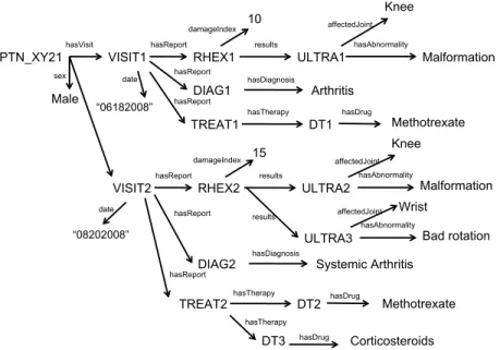
(16) Example 2. In Figure 8, Contexts(DrugT herapy, Diagnosis, P atient) = {V isit} because p1 = V isit.hasReport◦hasT herapy.DrugT herapy, p2 = V isit. hasReport.Diagnosis and p3 = P atient.hasV isit.V isit. Definition 5. Let i, i0 ∈ IS be two named instances. The expression (r1 ◦ · · · ◦ rn ) ∈ P aths(i, i0 ) is an aggregation path from i to i0 iff: 1. There exists a list of property assertions rj (ij−1 , ij ) ∈ IS, 1 ≤ j ≤ n. 2. There exists two concepts C, C 0 ∈ O such that O ∪ IS |= C(i) ∧ C 0 (i0 ) and (r1 ◦ · · · ◦ rn ) ∈ P aths(C, C 0 ) The first condition of the previous definition states that there must be a property chain between both instances in the IS, and the second one states that such a path must be also derived from the ontology. Definition 6. Let ia , ib ∈ IS be two named instances such that O ∪ IS |= Ca (ia ) ∧ Cb (ib ) ∧ Ca , Cb ∈ S ∧ Ca 6= Cb . Contexts(ia , ib , iSU B ) = S 0 ∀i0 ∈LCRI(ia ,ib ,iSU B ) {i }, where the function LCRI(ia , ib , iSU B ) returns the set of least common reachable instances, 1. |P aths(i0 , ia )| > 0 ∧ |P aths(i0 , ib )| > 0 ∧ |P aths(iSU B , i0 )| > 0 (i0 is common reachable instance). 2. @j ∈ IS such that j satisfies the condition 1 and |P aths(i0 , j)| > 0 (i0 is least). The previous definition is applied over instances belonging to different senses pairwise in order to find common contexts that relate them. Example 3. Figure 9 shows an example of IS represented as a graph that is consistent with ontology fragment in Figure 8. In this example, Contexts(DT 1, DIAG1, P T N XY 21) = {V ISIT 1} because p1 = V ISIT 1.hasReport ◦ hasT herapy.DT 1, p2 = V ISIT 1.hasReport.DIAG1 and p3 = P T N XY 21. hasV isit.V ISIT 1. Now, we can define which instances can be combined to each other for a certain analysis subject CSU B . Definition 7. Two instances ia , ib ∈ IS are combinable under a subject instance iSU B iff ∃ C1 ∈ {C(ix )/ix ∈ Contexts(ia , ib , iSU B )}, ∃ C2 ∈ Contexts( C(ia ), C(ib ), CSU B ) such that O |= C1 w C2 where C(i) is the asserted class for the instance i in IS. Example 4. As an example of the previous definition, let us check if instances DT 1 and DIAG1 of Figure 9 are combinable. In the definition, C1 can only be V isit and C2 is also V isit by looking at Figure 8. Since O |= V isit w V isit, instances DT 1 and DIAG1 are combinable under subject instance P T N XY 21. The intuition of the previous definition is that two instances are combinable only 16.

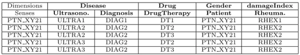
(17) hasVisit. PTN_XY21. hasReport. date. Male. “06182008”. affectedJoint hasAbnormality. results. VISIT1. sex. Knee. 10. damageIndex. RHEX1. ULTRA1. hasReport. hasDiagnosis. DIAG1. Arthritis. hasReport. hasTherapy. hasDrug. TREAT1. DT1. damageIndex. date. affectedJoint hasAbnormality. results. RHEX2 hasReport. Methotrexate Knee. 15. hasReport. VISIT2. Malformation. ULTRA2 affectedJoint. results. hasAbnormality. “08202008”. ULTRA3 DIAG2. hasDiagnosis. hasReport. TREAT2. hasTherapy. Malformation. Wrist Bad rotation. Systemic Arthritis. DT2. hasDrug. Methotrexate. hasTherapy. DT3. hasDrug. Corticosteroids. Figure 9: Example of instance store fragment consistent with ontology fragment of Figure 8.. if at the instance level (i.e., in the instance store or Abox) they appear under a context that belongs to or is more general than the context specified at the conceptual level (i.e., in the Tbox). Following this intuition, instances DT 1 and DIAG2 are not combinable because their contexts at the instance level are {P T N XY 21} whose type is P atient while at the conceptual level their contexts are {V isit}. This makes complete sense because the ontology has been defined in such a way that each visit contains the diseases diagnosed along with the drugs prescribed. Only valid combinations conformant with the MD schema are taken into account in the following definition. Definition 8. An instance context associated to iSU B ∈ IS is the tuple (i1 , · · · , in ), with n ≥ |D ∪ M |, satisfying the following conditions: 1. ∀c ∈ {D ∪ M }, there is at least one tuple element ix , 1 ≤ x ≤ n, such that O ∪ IS |= C(ix ) and C ∈ senses(c) or ix = N U LL otherwise. From now on, we will denote with dim(ix ) to the MD element associated to ix (i.e. c). 2. ∀(j, k), 1 ≤ j, k ≤ n, j 6= k, (ij , ik ) are combinable instances under iSU B . In other words, each of the elements of an instance context tuple is an instance that belongs to one sense and satisfies the combinable condition of Definition 7 with the rest of instances in the tuple. Therefore, an instance 17.

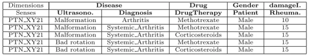
(18) Dimensions Senses PTN XY21 PTN XY21 PTN XY21 PTN XY21 PTN XY21. Disease Ultrasono. Diagnosis ULTRA1 DIAG1 ULTRA2 DIAG2 ULTRA2 DIAG2 ULTRA3 DIAG2 ULTRA3 DIAG2. Drug DrugTherapy DT1 DT2 DT3 DT2 DT3. Gender Patient PTN XY21 PTN XY21 PTN XY21 PTN XY21 PTN XY21. damageIndex Rheuma. RHEX1 RHEX2 RHEX2 RHEX2 RHEX2. Table 2: Instance context tuples generated for the running example. The second row accounts for the senses associated to each dimension.. context tuple represents all the potential valid interpretations from IS for a MD schema specification since all the elements of the MD schema must be covered by at least one instance or the N U LL value if there is not such instance (i.e. in case of optional values in the ontology). We say that an instance context tuple is ambiguous if there is more than one sense associated to the same dimension (measure). For example, tuples in Table 2 are ambiguous because the dimension Disease has associated two senses in all the tuples. Example 5. Given dimensions D = {Disease, Drug, Gender} and measures M = {damageIndex} with their associated senses, Table 2 shows the instance context tuples generated for subject instance P T N XY 21. Notice we keep track of the subject of analysis (i.e. Patient) in a new column.. Finally, we must project the intended values to obtain the facts that will populate the MD schema. Definition 9. A data fact associated to an instance context tuple (i1 , · · · , im ), is a tuple (d1 , · · · , dn ) with n ≥ m such that. dk =.    . jk. Q if dim(ik ) ∈ D and jk ∈ p (ik ) and O ∪ IS |= C(jk ) and C v dim(ik ) Q if dim(ik ) ∈ M and vk ∈ dim(ik ) (ik ) otherwise. vk null Q where p is the projection operation over an instance through the property   . p. Notice that we take into consideration that the projection can be multivalued (i.e. more than one value can be accessed with the same property in an instance). It is worth mentioning that “disambiguation” of instance tuples and data facts must be performed before building the OLAP cubes. Such a disambiguation can only be manually performed by the user according to her analysis requirements and the semantics involved. We will not treat further this issue as we consider it out of the scope of this paper.. 18.

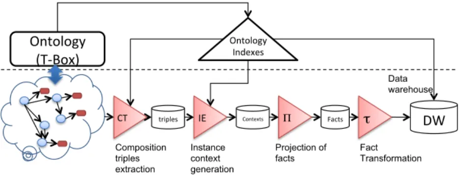
(19) Dimensions Senses PTN XY21 PTN XY21 PTN XY21 PTN XY21 PTN XY21. Disease Ultrasono. Diagnosis Malformation Arthritis Malformation Systemic Arthritis Malformation Systemic Arthritis Bad rotation Systemic Arthritis Bad rotation Systemic Arthritis. Drug DrugTherapy Methotrexate Methotrexate Corticosteroids Methotrexate Corticosteroids. Gender Patient Male Male Male Male Male. damageI. Rheuma. 10 15 15 15 15. Table 3: Data fact tuples generated for the running example.. Example 6. The previous instance context tuples in Table 2 give rise to the data fact tuples in Table 3 where each instance has been projected according to the previous definition. In the data fact tuples, measures are treated the same way as dimensions. Only when data fact tuples are going to be loaded into a cube, measure values sharing dimension values are aggregated according to the aggregation function selected.. Complexity Issues. In our method, the extraction of facts from the IS (Definition 9) requires the generation of different subsets of O (i.e. senses, paths and contexts), which in turn requires the use of a reasoner to perform inferences like O |= α and O ∪ IS |= α. The complexity of current reasoners depends on the expressiveness of both O and α, and consequently it directly affects to the efficiency of our method. It is worth mentioning that the expressivity of OWL DL leads to exponential complexity for these inferences. Fortunately, recently proposed OWL2 profiles (EL, QL and RL) have been demonstrated to be tractable for the main reasoning tasks (i.e. ontology consistency, class subsumption checking and instance checking). Additionally, definitions 4 to 8 require intensive processing over the inferred taxonomy of O and the underlying graph structure of IS. For this reason, we have designed a series of indexes and data structures aimed to efficiently perform the required operations. Next section is devoted to this issue. 5.2. Implementation The process of identification and extraction of valid facts from a semantic data repository involves several steps. In the previous section we have explained the identification of facts by means of a conceptual MD schema defined by the user. We have also lied down the foundations of valid facts from a semantic point of view. In this section we present an implementation for fact extraction that resembles ETL processes. Figure 10 sketches the steps involved in the fact extraction process. In the upper part of the figure we can see how ontology axioms (i.e., Tbox ) are indexed in order to handle basic entailments and hence minimizing the need of a reasoner. This task needs to be performed just once for each ontology and it can be done off-line. The on-line phase is shown in the bottom part of Figure 10. The first task consists of creating the composition triples from the instance store (i.e., Abox ) according to the user MD schema. These triples allow efficient 19.

(20) instance retrieval as well as reachability queries. Then, we generate instance context tuples (see Definition 8) from the composition triples with the help of the indexes. Since each context tuple can give rise to multiple facts, we project them over the desired attributes specified in the user MD schema, obtaining the intended data fact tuples (see Definition 9). Finally, we apply the required transformations over data fact tuples (e.g., normalizing or making partitions of numeric values). Next sections illustrate the index structures and their role in the fact extraction process.. Ontology (T‐Box). Ontology Indexes Data warehouse. CT. triples. Composition triples extraction. IE. Contexts. Instance context generation. Π. Facts. Projection of facts. τ. DW. Fact Transformation. Figure 10: ETL process for fact extraction.. 5.2.1. Ontology indexes We have designed two indexes over the ontology in order to handle basic entailments namely: is-a index and aggregation index. The is-a index is intended to efficiently answer concept subsumption queries and ancestors/descendants range queries. Briefly, the construction of the index involves the following steps: the TBox is normalized and completion rules are applied to make implicit subsumptions explicit. This process is similar to that presented in [14]. Then, all “is-a” relationships are modeled as a graph where nodes correspond to concepts and edges to “is-a” relationships. An interval labeling scheme able to encode transitive relations is applied to the graph. As a result, each node (i.e., concept) has assigned a descriptor that includes compressed information about its descendant and ancestor nodes in the form of intervals. Moreover, we provide an interval’s algebra over the node descriptors that allows performing basic DL operations over concepts. A detailed description of the indexing process and interval’s algebra can be found in [30]. The aggregation index is an index structure that allows answering reachability queries between concepts (see Definition 3). In order to construct this index, we apply the same interval labeling scheme as before over the ontology graph G = (V, L, E), where nodes in V are associated to the ontology classes, edge labels L represent the object property relation names and the “is-a” relation and edges e(v1 , v2 ) ∈ E represent the asserted relationships e ∈ L between nodes v1 , v2 ∈ V . By encoding descendants (i.e., reachable nodes following edge 20.

(21) direction) and ancestors (i.e., reachable nodes following inverse edge direction) for each node, we are able to encapsulate reachable nodes through both explicit and implicit aggregation paths. Going back to the graph fragment G showed in Figure 8, concept Drug has among its ancestors (i.e., reachable nodes) not only DrugTherapy and Treatment, but also Visit through inheritance of hasReport property of Visit. The operation Contexts(Ca , Cb , CSU B ) (see Definition 4) can be easily implemented using the aggregation index as follows: [. Contexts(Ca , Cb , CSU B ) =. (ancestors(C) ∪ C). C∈nca(Ca ,Cb )∩descendants(CSU B ). where operations nca, descendants and ancestors are efficiently performed through the interval’s algebra previously mentioned. 5.2.2. Instance store index The main purpose of the instance store (IS) index is to ease the task of finding out if two instances, or an instance and a literal, are connected in the instance store (see Definition 5). This index is materialized as composition triples. Definition 10. A composition triple is a statement of the form (s, o, p) where the subject (s) and object (o) are resources, and the predicate (p) is a composition path from the subject to the object. A composition path is an alternate sequence of properties and resources that connect both the subject and the object. For our purposes, the instance store index only keeps the composition triples that go from each instance of CSU B (i.e., the subject of analysis) to each of the instances i such that C(i) where C is a sense of the dimensions and measures. Moreover, both the subject and object of a composition triple contain a reference to their concept type C in the is-a index. Consequently, we can perform searches over the composition triples not only at the instance level (i.e., by exact matching of instance names in the subject and object) but also at the conceptual level (i.e., by specifying the subject and object concepts). The main operation defined over the composition triples is get instances(subject, path, object), where subject and object can be either a concept or instance, and path is a pattern matching string over the intended paths. Notice that the number of composition triples between two instances is equal to the number of unique paths in the IS graph for these instances. If the graph contains cycles, this number can be infinite. To avoid this problem, we assume that the IS forms a DAG, which indeed usually occurs in real world applications. We also require the composition path between a subject and an object to be unique. This way the number of composition triples is limited to |subjects| × |objects| and the relation between a subject and an object is unambiguous, avoiding possible summarizability issues in the resulting facts due to redundancy.. 21.

(22) Subject PTN XY21 PTN XY21 PTN XY21 PTN XY21 PTN XY21 PTN XY21 PTN XY21 PTN XY21 PTN XY21 PTN XY21 PTN XY21 PTN XY21 .... Composition Path /hasVisit /hasVisit /hasVisit/VISIT1/hasReport /hasVisit/VISIT1/hasReport/RHEX1/results /hasVisit/VISIT1/hasReport /hasVisit/VISIT1/hasReport/TREAT1/hasTherapy /hasVisit/VISIT2/hasReport /hasVisit/VISIT2/hasReport/RHEX2/results /hasVisit/VISIT2/hasReport/RHEX2/results /hasVisit/VISIT2/hasReport /hasVisit/VISIT2/hasReport/TREAT2/hasTherapy /hasVisit/VISIT2/hasReport/TREAT2/hasTherapy .... Object VISIT1 VISIT2 RHEX1 ULTRA1 DIAG1 DT1 RHEX2 ULTRA2 ULTRA3 DIAG2 DT2 DT3 .... Type Visit Visit Rheumatology Ultrasono. Diagnosis DrugTherapy Rheumatology Ultrasono. Ultrasono. Diagnosis DrugTherapy DrugTherapy .... Table 4: An excerpt of the composition triples of instance store fragment in Figure 9.. Table 4 shows an excerpt of composition triples for the IS fragment in Figure 9. The fourth column of the table shows the concept reference for the object. The concept reference for the subject is omitted because it is Patient for all the composition triples showed. 5.2.3. Instance Context & Data Fact Generation Our method to generate instance context tuples according to Definition 8, does not perform an exhaustive search over the instance store, since checking the combinable condition (see Definition 7) for each pair of instances would result in a combinatorial explosion. Instead, we use the ontology axioms to just select proper contexts that lead to valid combinations of instances. For this purpose we define the following data structure. Definition 11. Let O be an ontology (only the Tbox), CSU B the subject concept, DM = D ∪ M the set of dimensions and measures and S the set of senses of the dimensions and measures. The Contexts Graph ( CG) is a graph-like structure generated from O that satisfies the following conditions: 1. The root of the CG is CSU B . 2. The rest of the nodes of the CG are DM ∪ S ∪ {nd/ ∀Ci , Cj , 1 ≤ i, j ≤ |S|, Ci , Cj ∈ S, nd ∈ contexts(Ci , Cj , CSU B )}. 3. There is one edge from node ndi to node ndj iff |P aths(ndi , ndj )| > 0, @ ndk ∈ nodes(CG) such that |P aths(ndi , ndk )| > 0 ∧ |P aths(ndk , ndj )| > 0, where nodes(CG) denotes the set of nodes of CG. The generation of the CG is performed by calculating context nodes of the dimensions and measures senses. This process is supported by the operations provided by the aggregation index. Example 7. Given the conceptual MD schema of Example 5, the CG according to the previous definition is shown in the upper part of Figure 11, where shaded nodes act as contexts. The actual dimensions and measures are obviated for the sake of readability. 22.

(23) Algorithm 1 generates instance context tuples and uses the CG as a guide to process each subject instance (see Figure 11). The main idea is to process the CG in depth in order to recursively collect and combine instances under context node instances. They are collected with the operation gI(iSU B , path, CG node), where each output instance is a tuple and path is recursively constructed as the CG is processed, reflecting the actual path. Tuples are combined with the cartesian product until complete context tuples are obtained. The resulting instance context tuples are shown in Table 2. Data fact tuples are generated according to Definition 9 by projecting instances over the dimensions and measures. The resulting data fact tuples are shown in Table 3. Algorithm 1 Fact Extraction Algorithm Require: CG: contexts graph (as global var.), CT : composition triples (as global var.), iSU B = “ ∗ ”: subject instance, cpath = “ ∗ ”: composition path, CG node = CG.root: node from CG Ensure: ICT : valid instance context tuples (as global var.) 1: tuples = ∅ 2: Dvals = ∅ 3: Cvals = ∅ 4: instances = CT.get instances(iSU B , cpath, CG node) 5: for i ∈ instances do 6: if iSU B == “ ∗ ” then 7: iSU B = i 8: else 9: cpath = concatenate(cpath, i) 10: end if 11: for n ∈ CG.successors(CG node) do 12: if not CG.context node(n) then 13: v = CT.get instances(iSU B , cpath, n) 14: add(Dvals, v) 15: end if 16: end for 17: Dvals = cartesian product(Dvals) 18: for n ∈ CG.successors(CG node) do 19: if CG.context node(n) then 20: L = F act Extraction Algorithm(iSU B , cpath, n) 21: add(Cvals, L) 22: end if 23: end for 24: Cvals = combine(Cvals) 25: combs = cartesian product(Dvals, Cvals) 26: if CG.is root node(CG node) then 27: add(ICT, combs) 28: else 29: add(tuples, combs) 30: end if 31: end for 32: return tuples. 6. Extracting Dimensions Once instance facts are extracted, the system can proceed to generate hierarchical dimensions from the concept subsumption relationships inferred from the ontology. These dimensions, however, must have an appropriate shape to. 23.

(24) Contexts Graph. Pa6ent. Visit. Diagnosis. gI(PTN XY21, `*/VISIT1/*’,Rheumatology). gI(PTN XY21, `*/VISIT1/*/RHEX1/*’,DrugTherapy). gI(PTN XY21, `*/VISIT2/*’,Rheumatology). gI(PTN XY21, `*/VISIT2/*/RHEX2/*’,DrugTherapy). gI(PTN XY21, `*/VISIT1/*', Diagnosis). gI(PTN XY21, `*/VISIT1/*/RHEX1/*’,Ultrasonography). gI(PTN XY21, `*/VISIT2/*', Diagnosis) gI(‘*’, ‘*’,Patient). PTN XY21. DrugTherapy. Ultrasonography. Rheumatology. gI(PTN XY21, `*/VISIT2/*/RHEX2/*’,Ultrasonography). gI(PTN XY21, `*', Visit) VISIT1. ×. DIAG1. ×. RHEX1. ×. VISIT2. ×. DIAG2. ×. RHEX2. ×. ×. ULTRA1 ULTRA2 ULTRA3. × ×. DT1 DT2 DT3. Figure 11: Contexts graph processing along with the generation of context tuples for instance store of Figure 9. Shaded nodes correspond to contexts. Function gI is the short name for function get instances.. perform properly OLAP operations. Therefore extracted hierarchies must comply with a series of constraints to ensure summarizability [22]. In this section, we propose a method to extract “good” hierarchies for OLAP operations from the ontologies in the repository, but preserving as much as possible the original semantics of the involved concepts. In this work we only consider taxonomic relationships, leaving as future work other kind of relationships (e.g. transitive properties, property compositions, etc.), which have been previously treated in the literature [34]. 6.1. Dimension Modules The first step to extract a hierarchical dimension Di consists of selecting the part of the ontology that can be involved in it. Let Sig(Di ) be the set of most specific concepts of the instances participating in the extracted facts (see Definition 9). We define the dimension module MDi ⊆ O as the upper module of the ontology O for the signature Sig(Di ). We define upper modules in the same way as in [21, 23, 30], that is, by applying the notion of conservative extension. Thus, an upper module M of O for the signature Sig is a sub-ontology of O such that it preserves all the entailments over the symbols of Sig expressed in a language L, that is, O |= α with Sig(α) ⊆ Sig and α ∈ L iff MDi |= α. For OLAP hierarchical dimensions we only need to preserve entailments of the form C v D and C disjoint D, being C and D named concepts. Thus, the language of entailments corresponds to the typical reasoners output. This kind of upper modules can be extracted very efficiently over very large ontologies [30].. 24.

(25) 6.2. Dimension Taxonomies Let T AX(MDi ) be the inferred taxonomy for the module MDi , which is represented as the directed acyclic graph (DAG) (V, E), where V contains one node for each concept in MDi , and ci → cj ∈ E if ci is one of the least common subsumers of cj (i.e. direct ancestor). T AX(MDi ) is usually an irregular, unbalanced and non-onto hierarchy, which makes it not suitable for OLAP operations. Therefore, it is necessary to transform it to a more regular, balanced and tree-shaped structure. However, this transformation is also required to preserve as much as possible the original semantics of the concepts as well as to minimize the loss of information (e.g. under-classified concepts). Former work about transforming OLAP hierarchies [33] proposed the inclusion of fake nodes and roll-up relationships to avoid incomplete levels and double counting issues. Normalization is also proposed as a way to solve non-onto hierarchies [26]. These strategies however are not directly applicable to ontology taxonomies for two reasons: the number of added elements (e.g. fake nodes or intermediate normalized tables) can overwhelm the size of the original taxonomy and, the semantics of concepts can be altered by these new elements. Recently, [15] proposes a clustering-based approach to reduce taxonomies for improving data tables summaries. This method transforms the original taxonomy to a new one by grouping those nodes with similar structures and usage in the tuples. However, this method also alters the semantics of the symbols as new ones are created by grouping original ones. 6.3. Selecting good nodes Similarly to our previous work about fragment extraction [30], we propose to build tailored ontology fragments that both preserve as much as possible the original semantics of the symbols in Sig(Di ) and present a good OLAPlike structure. For the first goal, we will use the upper modules MDi as the baseline for the hierarchy extraction. For the second goal, we propose a series of measures to decide which nodes deserve to participate in the final hierarchy. Before presenting the method, let us analyze why T AX(MDi ) presents such an irregular structure. The usage of symbols in Sig(Di ) can be very irregular due to the “popularity” of some symbols (i.e. Zipf law), which implies that few symbols are used very frequently whereas most of them are used few times. As a result, some parts of the taxonomy are more used than others, affecting to both the density (few dense parts and many sparse parts) and the depth of the taxonomy (few deep parts). A direct consequence is that some concepts in Sig(Di ) are covered by many spurious concepts which are only used once, and therefore are useless for aggregation purposes. So, our main goals should be to identify dense regions of the taxonomy and to select nodes that best classify the concepts in Sig(Di ). The first measure we propose to rank the concepts in T AX(MDi ) is the share: share(n) =. Y ni ∈ancs(n). 25. 1 |children(ni )|.

(26) where ancs(n) is the set of ancestors of n in T AX(MDi ), and children(n) is the set of direct successors of n in the taxonomy. The idea behind the share is to measure the number of partitions produced from the root till the node n. The smaller the share the more dense is the hierarchy above the node. In a regular balanced taxonomy the ideal share is S(n)depth(n) , where S is the mean of children the ancestor nodes of n have. We can then estimate the ratio between the ideal share and the actual one as follows: ratio(n) =. S(n)depth(n) share(n). Thus, the greater the ratio, the better the hierarchy above the node is. The second ranking measure we propose is the entropy, which is defined as follows: entropy(n) = Σni ∈children(n) Psig (n, ni ) · log(Psig (n, ni )) Psig (n, ni ) =. coveredSig(ni ) coveredSig(n). where coveredSig(n) is the subset of Sig(Di ) whose members are descendants of n. The idea behind the entropy is that good classification nodes are those that better distribute the signature symbols among its children. Similarly to decision trees and clustering quality measures, we use the entropy of the groups derived from a node as the measure of their quality. In order to combine both measures we just take the product of both measures: score(n) = entropy(n) · ratio(n) 6.4. Generating hierarchies The basic method to generate hierarchies consists of selecting a set of “good” nodes from the taxonomy, and then re-construct the hierarchy by applying the transitivity property of the subsumption relationship between concepts. Algorithm 2 presents a global approach, which consists of selecting nodes from the nodes ranking until either all signature concepts are covered or there are no more concepts with a score greater than a given threshold (usually zero). Alternatively, we propose a second approach in Algorithm 3, the local approach, which selects the best ancestors of each concept leaf of the taxonomy. In both approaches, the final hierarchy is obtained by extracting the spanning tree that maximizes the number of ancestors of each node from the resulting reduced taxonomy [30]. One advantage of the local approach is that we can further select the number of levels up to each signature concept, defining so the hierarchical categories for the dimensions. However, this process is not trivial and we decided to leave it for future work. Each method favors different properties of the 26.

(27) generated hierarchy. If the user wants to obtain a rich view of the hierarchy, she must select the global one. Instead, if the user wants a more compact hierarchy (e.g., few levels) then she must select the local one. Algorithm 2 Global approach for dimension hierarchy generation Require: the upper module (MDi ) and the signature set (Sig(Di )) for dimension Di . Ensure: A hierarchy for dimension Di . Let Lrank be the list of concepts in MDi ordered by score(n) (highest to lowest); Let F ragment = ∅ be the nodes set of the fragment to be built. repeat pop a node n from Lrank add it to F ragment S until score(n) ≤ 0 or n∈F ragment coveredSig(n) == Sig(Di ) Let N ewT ax be the reconstructed taxonomy for the signature F ragment return spanningT ree(N ewT ax). Algorithm 3 Local approach for dimension hierarchy generation Require: the upper module (MDi ) and the signature set (Sig(Di )) for dimension Di . Ensure: A hierarchy for dimension Di . Let Lleaves be the list of leaf concepts in MDi ordered by ratio(n) (highest to lowest); Let F ragment = ∅ be the nodes set of the fragment to be built. for all c ∈ Lleaves do Set up Lancs (c) with the ancestors of c ordered by score(n) for all na ∈ Lancs (c) do if there is no node n2 ∈ Lancs (c) such that score(n2 ) ≤ score(na ) and order(n2 ) ≤ order(na ) then if na ∈ / F ragment then add na to F ragment end if end if end for end for Let N ewT ax be the reconstructed taxonomy for the signature F ragment return spanningT ree(N ewT ax). 7. Evaluation We have conducted the experiments by applying our method to a corpus of semantic annotations about rheumatic patients. The experimental evaluation has two differentiated setups. On one hand, we are concerned with scalability and performance issues regarding the generation of facts from the analyst requirements. On the other hand, we evaluate the two proposed methods for generating dimensions from the ontology knowledge by measuring the quality of the resulting hierarchies. 7.1. Fact extraction The dataset used for the fact extraction evaluation has been synthetically generated from the features identified from a set of real patients. For this purpose, we have extended the XML generator presented in [36] with new operators. 27.

(28) global. original X 9 5. 9. 9. 0. 0. 0 5. 6 7 8. 1 2 3 4. 5. 6 7 8. 6 7 8. 1 2 3 4. 1 2 3 4. (b). (a) ancestors. local 9. 9 0. 5. 5. (a). 1 2. 3 4 6 7 8. 1 2 3 4. 6 7 8. (b). Figure 12: Example of local and global methods: (a) node selection and (b) hierarchy reconstruction. Dashed edges in (b) are removed in the final spanning tree. Nodes inside squares in (b) are those that change its parent in the resulting dimension.. specific for RDF/OWL. The Tbox template has been carefully designed following the structure of the medical protocols defined in the Health-e-Child5 project for rheumatic patients. Moreover, domain concepts are taken from UMLS. With the previous setup, we are able to generate synthetic instance data of any size and with the intended structural variations to account for heterogeneity and optional values of semantic annotations. In particular, the dataset contains more than half million of instances. Figure 13 presents how the number of elements in the MD schema (i.e. number of dimensions and measures) affects the time performance to generate the fact table with all valid combinations of instances (i.e. data fact tuples). For the experiment setup we have preselected a set of 11 candidate dimensions and measures from the ontology and have computed all the fact tables that can be generated from all subsets of these 11 elements. The total number of fact tables is 211 = 2048. Then, we have organized the fact tables according to the number of dimensions and measures in their MD schema (x axis), from two dimensions to eleven. Axis y shows the time performance in seconds. Each boxplot in the figure shows the variance in time between fact tables having the same number of dimensions and measures. The explanation for this variance is that different MD configurations of the same size may obtain very different CGs depending on their structural dependencies. Therefore, the number of instances processed 5 http://www.health-e-child.org/. 28.

(29) Figure 13: Fact table generation performance w.r.t. the number of dimensions and measures involved.. and the levels of recursion are different, resulting in different processing times. In general, the time complexity increases linearly with respect to the number of dimensions and measures of the fact table, which proves the scalability and efficiency of the approach. On the other hand, we are also concerned about how the size of the instance store affects the generation of the fact tables. Figure 14 illustrates the results. From the previous experiment we have selected one of the smallest (i.e., 2 elements) and the largest (i.e., 11 elements) MD schema specification. For these two MD configurations we measure the time to create the respective fact tables with instance stores of different sizes, ranging from 100 to 3000 complex instances of type P atient. Notice axis x measures the number of subject instances, although the number of total instances in the store ranges from a thousand to more than half million instances. For both configurations, the time performance is linear w.r.t. the size of the instance store, which means the method proposed is scalable. 7.2. Dimensions extraction In order to measure the quality of the dimension hierarchies obtained with the methods proposed in Section 6 (i.e. global vs. local), we have adapted the measures proposed in [15], namely dilution(Di , F ragment, T ) =. 1 X ∆O (parentO (t[Di ]), parentF ragment (t[Di ])) |T | t∈T. diversity(Di , F ragment, T ) =. (|T |2. 2 − |T |) 29. X t1 ,t2 ∈T,t1 6=t2. ∆F ragment (t1 [Di ], t2 [Di ]).

(30) 150 0. 50. time (s). 100. Smallest MD schema Largest MD schema. 0. 500. 1000. 1500. 2000. 2500. 3000. # topic instances. Figure 14: Increase in the time complexity w.r.t. the size of the instance store.. where T is the fact table, hits(T, ni ) is the times ni has been used in T , parentO (n)6 is the parent of n in O, and ∆O is the taxonomic distance between two nodes in O. t[Di ] represents the concept assigned to the fact t for the dimension Di . Dilution measures the weighted average distance in the original taxonomy between the new and original parents of the signature concepts from dimension Di . The weight of each signature concept corresponds to its relative frequency in the fact table. The smaller the dilution, less semantic changes have been produced in the reduced taxonomy. Diversity measures the weighted average distance in the reduced taxonomy of any pair of concepts from dimension Di used in the fact table. The greater the diversity, better taxonomies are obtained for aggregation purposes. A very low diversity value usually indicates that most concepts are directly placed under the top concept. We have set up 25 signatures for 14 dimensions of the dataset described in the previous section. The size of these signatures ranges from 4 to 162 concepts (60 on average). The corresponding upper-modules are extracted from UMLS following the method proposed in [29]. The size of these modules ranges from 40 to 911 concepts (404 on average). Their inferred taxonomies present between 8 and 23 levels (17 on average). Results for the global and local methods are 6 Indeed, we assume that the parent of n in O is the parent in the extracted spanning tree of O.. 30.

(31) Measure Reduction (%) Sig. Lost (%) Dilution Diversity. Global 72.5 - 75.9 7.08-12.12 0.367-0.473 9.08-10.79. Local 76.5 - 79.8 3.5-7.8 0.342-0.429 7.72-9.46. Table 5: Results for global an local dimension extraction methods. Value ranges represent the 0.75 confidence intervals of the results for all the signatures.. shown in Table 5. From these results we can conclude that: (1) the local method generates smaller dimension tables, (2) the local method implies less signature lost, but dilution values of both methods are not statistically different and, (3) diversity is usually greater in the global method (i.e. richer taxonomies are generated). To sum up, each method optimizes different quality parameters, and therefore their application will depend on the user requirements. 7.3. Implementation We use M ySQL7 database as back-end to store the semantic annotations (i.e. ABox), the domain and application ontologies (i.e. T Box) and the required indexes. On the other hand, we use the Business Intelligence (BI) tool of Microsoft SQL Server 2008 8 to instantiate the MD schema designed by the user and create cubes. Our method is completely independent of any data management system. We simply need to create an API to the back-end where the information is stored and the populated MD schema is delivered as a series of tables that can be fed into any off the shelf analysis tool. In Figure 15 we show the result of one of the MD queries proposed for the use case in section 2.2. In this use case, the user is interested in analyzing the efficacy of different drugs w.r.t. a series of dimensions, such as the disease diagnosed, the patient’s age, gender, etc. The method first generates the fact table according to the conceptual MD schema proposed by the analyst and then, for each dimension, a dimension hierarchy is extracted using the global approach. The result (i.e. the populated MD schema) has been fed to SQL Server and the BI tool allows the analyst to create cubes and navigate through them. In particular, Figure 15 shows the cube generated by averaging the damageIndex measure by disease (rows) and drug (columns). As shown, the user can navigate through the different levels of the dimension hierarchies and the measures are automatically aggregated. It is worth mentioning the added value that provides the semantics involved in the aggregations, since the dimension hierarchies express conceptual relations extracted from a domain ontology. 7 MySQL: 8 SQL. http://www.mysql.com Server 2008: http://www.microsoft.com/sqlserver/2008. 31.

(32) Figure 15: Example of MD cube created by averaging the damageIndex measure by disease (rows) and drug (columns).. 8. Related work Although there is a significant amount of literature that relates to different aspects of our approach (e.g. SW, MD models, OLAP analysis, etc.), there is little or no research that addresses the analysis of semantic web data (i.e. RDF/(S) and OWL) by using the above-mentioned technologies. However, we find worth reviewing some work on querying and analysis over heterogeneous XML data, which is the standard on which SW languages rely on. Some research has focused on querying complex XML scenarios where documents have a high structural heterogeneity. In [25, 41] it is shown that XQuery is not the most suitable query language for data extraction from heterogeneous XML data sources, since the user must be aware of the structure of the underlying documents. The lowest common ancestor (LCA) semantics can be applied instead to extract meaningful related data in a more flexible way. [25, 41] apply some restrictions over the LCA semantics. In particular they propose SLCA [41] and MLCA [25] whose general intuition is that the LCA must be minimal. However, in [28, 32] they showed that these approaches still produced undesired combinations between data items in some cases (e.g. when a data item needs to be combined with a data item at a lower level of the document hierarchy). In order to alleviate the previous limitations they propose the SPC (smallest possible context) data strategy, which relies on the notion of closeness of data item occurrences in an XML document. There exists other strategies to extract transactions or facts from heterogeneous XML [38]. However, they are used in data mining applications and they do not care for OLAP properties such as “good” dimensions and summarizability issues. We face similar challenges as the previous approaches mainly due to the structural heterogeneity of the semantic annotations. However, we still need to deal with the semantics, which requires logical reasoning in order to derive implicit information. Other approaches such as [34, 35] try to incorporate semantics in the design of a data warehouse MD schema by taking as starting point an OWL ontology that describes the data sources in a semi-automatic way. Instead of looking for functional dependencies (which constitute typical fact-dimension relations) in the sources, they are derived from the ontology. However, this work focuses on the design phase, overlooking the process of data extraction and integration to populate the MD schema. This issue is partially addressed in [24] by using SPARQL over RDF-translated data sources. However, this is not appropriate 32.

(33) for expressive and heterogeneous annotations. By combining IE techniques with logical reasoning, in [18] they propose a MD model specially devised to select, group and aggregate the instances of an ontology. In our previous work [31] we define the semantic data warehouse as a new semi-structured repository consisting of semantic annotations along with their associated set of ontologies. Moreover, we introduce the multidimensional integrated ontology (MIO) as a method for designing, validating and building OLAP-based cubes for analyzing the stored annotations. However, the fact extraction and population is pointed out in a shallow way and it is the main concern of the current paper. 9. Conclusions More and more semantic data are becoming available on the web thanks to several initiatives that promote a change in the current Web towards the Web of Data, where the semantics of data become explicit through data representation formats and standards such as RDF/(S) and OWL. However, this initiative has not yet been accompanied by efficient intelligent applications that can exploit the implicit semantics and thus, provide more insightful analysis. In this paper, we investigate how semantic data can be dynamically analyzed by using OLAP-style aggregations, navigation and reporting. We propose a semi-automatic method to build valid MD fact tables from stored semantic data expressed in RDF/(S) and OWL formats. This task is accomplished by letting the user compose the conceptual MD schema by selecting domain concepts and properties from the ontologies describing the data. Dimension hierarchies are also extracted from the domain knowledge contained in the ontologies. The benefits of our method are numerous, however we highlight the following: 1) we provide a novel method to exploit the information contained in the semantic annotations, 2) the analysis is driven by the user requirements and it is expressed always at the conceptual level, 3) the analysis capabilities (i.e. the OLAP-style aggregations, navigation, and reporting) are richer and more meaningful, since they are guided by the semantics of the ontology. To our knowledge, this is the first method addressing this issue from ontological instances. Hence, we do believe this work opens new interesting perspectives as it bridges the gap between the DW and OLAP tools and SW data. As future work, we plan to improve the method in several aspects. In particular, we plan to extend the local method for generating dimension hierarchies so that the dimension values can be grouped into a defined number of levels or categories. We are also working on an extended conceptual MD specification for the analyst in terms of richer ontology axioms. Regarding performance issues, a promising direction is the application of bitmap indexing techniques to SW data management, including efficient reasoning. Finally, we are also concerned about different SW scenarios where the development of the ontology axioms and the instance store is not coupled. In such scenarios, we need to study how to treat the possible vagueness of the ontology axioms (or even absence) w.r.t. to the instance store, which hinders the proposed extraction of facts.. 33.