Notes on international volatility for the country studies

Texto completo

(1)cedes. Nuevosdocumentos. 2005/17 área economía. NOTES ON INTERNATIONAL VOLATILITY FOR THE COUNTRY STUDIES Project: International Financial Architecture, Macro Volatility, and Institutions. The Developing World Experience. José María Fanelli Coordinator of the Project. Eduardo Corso provided superb research assistance. I thank Ariel Geandet for his useful comments. Sánchez de Bustamante 27. 1173 Buenos Aires / Argentina. (54-11) 4861-5204 / Fax: 4862-0805. www.cedes.org.

(2) These notes present and analyze data on international aggregate volatility. Their purpose is to identify a set of stylized facts to be used as a benchmark for the country studies that are being prepared for the project: “International Financial Architecture, Macro Volatility, and Institutions. The Developing World Experience.” The project has two central hypotheses: first, there are complex causal connections between aggregate volatility and institutional weaknesses; second, developing countries show excessive aggregate volatility. The rationale behind these hypotheses is that weak institutions generate excess volatility because institutional flaws place strict limits on the ability of both private agents and governments to manage risk. More precisely, we argue that under weak institutional conditions, some risks are not contractible and certain risk-smoothing policies are not implementable. We further argue that, as a consequence, there will exist a set of mutually advantageous transactions that will not be undertaken; the market structure will thus be incomplete; and, the policies to manage the effects of market and coordination failures will not be efficient. Under these conditions risk will not be allocated optimally and there will be "excess" volatility in the system. The risk-bearing costs will exceed those justified by fundamentals (see the background paper for an indepth discussion of this point). In line with this approach, our search for stylized facts focuses on: one, the characterization of aggregate volatility in developing countries; two, the identification of observable and measurable consequences of the interactions between institutions and aggregate volatility; and, three, the detection and measuring of excess volatility. To do so, we need an operational measure of aggregate volatility, a standard to assess the size of excess volatility, and indicators reflecting the volatility-institutions’ interactions. The most popular measure of volatility in the literature on international volatility is the standard deviation of the variable under consideration. This implies identifying volatility with the total variability of the variable. Given that total variability comprises both anticipated and unanticipated movements of the variable, some authors disagree with this approach. They argue that only unanticipated movements matter from the point of view of risk-related decisions. A good part of the empirical literature, nonetheless, does not take into account this distinction. Furthermore, in the background paper we argued that this is not necessarily wrong because the assertion that we should focus on unanticipated movements to assess the costs of volatility is true only in a complete-market setting. When some contracts cannot be written because of institutional flaws, not only unanticipated but also anticipated cyclical movements can impose costs on the economy. That is, even if agents were able to anticipate the movement of a certain variable and knew exactly what their best response would be, they would not be able to undertake all the necessary transactions required to implement their decisions if some markets were missing. This means that anticipated movements and, hence, total variability may have a bearing on the generation of costs associated with excess volatility.. 1.

(3) In line with the usual practice in the literature (although perhaps for slightly different reasons), our basic volatility measure will be the standard deviation of the continuous growth rate of the variable under analysis. We will try to identify the costs of excess volatility irrespective of whether they stem from anticipated or unanticipated movements of the relevant variables, which means that not only uncertainty but also market and policy failures will be considered, in principle, relevant to explaining the burden aggregate volatility imposes on society. The election of the standard to measure the costs of excess volatility is no less challenging. One possibility is to benchmark the amount of volatility observed against the amount of "fundamental" volatility predicted by the complete-market theoretical model. However, once institutions are introduced into the picture, assessing the extent to which markets are “missing” thus producing excess volatility costs is, nonetheless, a complicated task. To begin with, from a Coasian perspective, it is not possible to tell a priori whether markets or firms will be responsible for allocating specific risks. This depends on transactions costs, which in turn, depends on institutions that are somewhat endogenous. We cannot use the complete-market theoretical benchmark to tackle this problem because the institutional structure and transaction costs are not specified in the theoretical model1. In light of these analytical constraints, we have adopted a pragmatic two-step strategy. First, we will use the main predictions of the perfect-market theoretical paradigm as a guide for detecting the presence of excessive costs of risk in our aggregate data. Second, in order to measure the “size” of such costs in the case of developing countries, we will take developed economies rather than the theoretical model as our benchmark. That is, given that we assume that developing countries’ risk management is flawed because market options to allocate risks are reduced and the policy sophistication is limited, it is reasonable to assume that the amount of excess aggregate volatility should be the lowest in those countries in which the level of financial deepening and the quality of policies is the highest. Although the comparison with the developed-country benchmark does not tell us how far a certain developing economy is from a first-best situation, it does tell us how much excess volatility could, in principle, be eliminated if developing countries markets and institutions were to become as strong as they currently are in developed countries. Data availability placed severe constraints on our ability to test hypotheses and measure aggregate volatility. Furthermore, it is very difficult to identify the different sources of volatility costs based on observations of the volatility of aggregate variables. We will concentrate on detecting the presence and assessing the importance of excess volatility costs in developing countries rather than on identifying precisely their 1. A second difficulty is that excess volatility costs can take the form of lower rather than higher volatility of real and financial variables. That is, if agents cannot insure certain risks, they may avoid undertaking risky projects and the observational consequence will be a lower rather than a higher volatility of output. These effects operate basically at the micro level. Given that we are going to work with aggregate data, we cannot identify them. In the background paper, nonetheless, we discussed the reasons why the analytical and empirical evidence strongly suggests that excess volatility costs take the form of excess aggregate volatility, the main cause being that the lack-of-diversification effect dominates at the aggregate level. Note that the test for the presence of excess volatility costs in developing countries would be to find simultaneously more sectoral volatility and less aggregate volatility in developed countries. And this is, in fact, the case (see the background paper).. 2.

(4) different sources. From this point of view, our work should be considered heuristic. In fact, it is precisely because of the limitations of panel data techniques and the poor quality of international data sets that the project largely relies on country studies to disentangle and characterize the causal links between aggregate volatility and institutions, to examine the sources of shocks, and the operation of amplification/dampening mechanisms. Our work concentrates on hypotheses involving consumption and output volatility because they enjoy comparative advantages for two reasons: greater availability of internationally comparable data and high theoretical relevance. In light of this, although we will study a number of volatility indicators, our search for detecting and assessing excess volatility will focus on output and consumption volatility. The first section presents evidence on international GDP and private consumption volatility and the second studies the behavior of a set of indicators that can be exploited to detect the presence of excess volatility stemming from failures in financial markets. We focus on the volatility of the terms of trade, imports, exports, and capital flows. We also analyze the role of trade openness, domestic financial deepening, and macroeconomic persistence as an indicator of the characteristics of the contract structure. The third section addresses the detection and measurement of excess volatility costs and presents the main conclusions.. 3.

(5) I. Measuring International GDP and Consumption Volatility The aggregate volatility measures will be based on observations of the GDP2, aggregate private consumption, and other key volatility indicators–such as terms of trade, and capital movements–for the period 1960-2002. Our basic sample comprises 81 countries, although under certain circumstances the number of countries in the sample will be lower because of data problems. We utilize the World Development Indicators data base (World Bank, 2004). 1. GDP Growth Volatility Figure 1 displays the volatility of GDP for different regions of the world and different levels of GDP per capita–in increasing order–for the period 1960-2002. As data for the group of former socialist countries is unavailable for the entire 1960-2002 period, the volatility measures corresponding to these countries are based on more recent data (the nineties). 0.12. Figure 1: GDP Volatility by per capita GDP (1960-2002). 0.1. GDP Volatility. 0.08. 0.06. 0.04. 0.02. Malawi Burundi China Burkina Faso Nigeria India Rwanda Bangladesh Kenya Madagascar Leshoto Pakistan Gambia Togo Benin Ghana Mauritania Indonesia Zambia Zimbabwe Senegal Nicaragua Cameroon Honduras Congo Egypt, Arab. Cote D'Ivory Phillipines Morocco Thailand Ukraine Dominican Guatemala Algeria Paraguay Tunisia Ecuador Bulgaria Romania Colombia Malaysia Peru Mexico Costa Rica Chile Poland Russia Brazil Hungary Trinidad and T. South Africa Slovak Republic Gabon Korea Uruguay Czech Republic Argentina Portugal Greece Spain Hong Kong Ireland Italy New Zeland United Kingdom Australia Canada Finland Iceland Belgium France Netherlands Austria United States Norway Sweden Germany Japan Denmark Luxembourg Switzerland. 0. Source: World Develompment Indicators.. The figure suggests that growth volatility tends to be higher in the developing world. In Figure 2 we have plotted income volatility against per capita GDP. This graph also suggests that GDP volatility and per capita income are associated.. 2. We could also use GNP. However, GDP and GNP are highly correlated and GDP measures appear to be more reliable than GNP in developing countries (see Obstfeld, 2004).. 4.

(6) Figure 2: Per Capita GDP and GDP volatility (1960-2002). 0.12. GDP Volatility. 0.1. 0.08. 0.06. 0.04. 0.02. 0 4. 5. 6. 7. 8. 9. 10. 11. Per Capita GDP (log). Source: World Develompment Indicators.. Aggregate volatility, nonetheless, exhibits substantial differences across regions and over time. Figure 3 shows the evolution of each country’s volatility by region and Table 1 records average volatility by region and by period. We consider two different international scenarios –pre-globalization (1960-1989) and globalization (1990-2002). The first scenario includes two architectures: the Bretton Woods regime (1960-1971) and the period in which the regime melted and disappeared (1972-1989), characterized by floating exchange rates and two oil crises. Of course, the election of the years for regime change is to a certain extent arbitrary. However, given the importance of the changes in the international financial architecture for our project, it is worth examining. Figure 3a: GDP Volatility. (1960-1989) vs. (1990-2002) OECD Countries.. 0.2 0.18 0.16. GDP Vol (1960-1989). 0.14. GDP Vol (1989-2002). 0.12 0.1 0.08 0.06 0.04 0.02. United States. Switzerland. Spain. Sweden. Norway. Portugal. New Zeland. Mexico. Netherlands. Korea. Luxembourg. Italy. Japan. Ireland. Iceland. United Kingdom. Source: World Develompment Indicators.. Greece. France. Germany. Finland. Canada. Denmark. Austria. Belgium. Australia. 0. 5.

(7) Figure 3b: GDP Volatility. (1960-1989) vs. (1990-2002) Euro Area. 0.2 0.18. GDP Vol (1960-1989). 0.16. GDP Vol (1989-2002). 0.14 0.12 0.1 0.08 0.06 0.04 0.02. Source: World Develompment Indicators.. Spain. Portugal. Netherlands. Luxembourg. Italy. Ireland. Greece. Germany. France. Finland. Belgium. Austria. 0. Figure 3c: GDP Volatility. (1960-1989) vs. (1990-2002) Latin American Countries.. 0.2 0.18 0.16. GDP Vol (1960-1989). 0.14. GDP Vol (1989-2002). 0.12 0.1 0.08 0.06 0.04 0.02. Mexico. Uruguay. Peru. Paraguay. Nicaragua. Honduras. Guatemala. El Salvador. Ecuador. Trinidad and T.. Source: World Develompment Indicators.. Dominican R.. Costa Rica. Colombia. Chile. Brazil. Argentina. 0. Figure 3d: GDP Volatility. (1960-1989) vs. (1990-2002) African Countries.. 0.2 0.18. GDP Vol (1960-1989). 0.16. GDP Vol (1989-2002). 0.14 0.12 0.1 0.08 0.06 0.04 0.02. Zambia. Zimbabwe. Tunisia. Togo. Senegal. South Africa. Nigeria. Rwanda. Morocco. Mauritania. Malawi. Madagascar. Kenya. Leshoto. Ghana. Gambia. Gabon. Cote D'Iv.. Egypt, A. R.. Congo. Cameroon. Burundi. Burkina F.. Benin. Algeria. 0. Source: World Develompment Indicators.. 6.

(8) Figure 3e: GDP Volatility. (1960-1989) vs. (1990-2002) Asian Countries.. 0.2 0.18 0.16. GDP Vol (1960-1989). 0.14. GDP Vol (1990-2002). 0.12 0.1 0.08 0.06 0.04 0.02. Korea. Japan. Thailand. Singapore. Phillipines. Pakistan. Malaysia. Indonesia. India. Hong Kong. China. Bangladesh. 0. Source: World Develompment Indicators.. Figure 3f: GDP Volatility. Transition Countries. (1990-2002). 0.2 0.18 0.16 0.14 0.12 0.1 0.08 0.06 0.04 0.02. Ukraine. Slovak Republic. Romania. GDP Vol (1989-2002). Russian Federation. Source: World Develompment Indicators.. Poland. Hungary. Czech Republic. Bulgaria. 0. Figures 3a to 3f indicate that the former socialist countries and the African economies tend to be the most volatile, followed by the countries in the Latin American and Asian regions. The OECD members and the countries in the European Monetary Union are much less volatile. In addition, it seems that there is a tendency for GDP volatility to fall under globalization.. 7.

(9) Table 1: Mean GDP Growth Volatility by Region and Period (%) Region. Mean Volatility Mean Volatility p-value Period 1960-1989 1990-2002 vs. Period.. Euro Area. 2.6. 1.9. 8. OECD. 2.6. 2.4. 66.6. Africa. 5.7. 3.9. 0.9. Asia. 3.9. 3.2. 37.9. Latin America. 4.5. 3.3. 4.5. Transition. ----. 6.7. ---. Table 1 confirms that there is a fall in mean volatility in all regions under globalization, although the fall in some cases is very small and, additionally, there are important differences in the volatility levels across regions during Bretton Woods, as well as during the globalization period. To assess the statistical significance of the fall in volatility, the last column of Table 1 displays the results of a mean equality test. The null hypothesis states that no change in mean volatility exists between the first and the second period. If the reported p-value is less than the size of the test, say 5%, the null hypothesis should be rejected. According to this test, there has been a significant fall in volatility in Africa, Latin America, and the European Monetary Union (in this case the p-value is 8%) while Asia and the OECD countries have experienced no changes in volatility as the world underwent an increasing globalization process. Table 2: Testing for Differences in Regional Volatility Region. p-value Regions vs. Developed. p-value Regions vs. Euro Area. p-value Regions vs. Emerging. Euro Area. 55.2. --. 0.0. OECD. 13.4. 17.1. 0.1. Africa. 0.0. 0.0. 0.9. Asia. 0.2. 0.6. 12.8. Latin America. 0.0. 0.1. 53.8. Transition. 0.0. 0.0. 5.1. Table 2 shows the results of testing whether regional differences in mean volatility are significant. We use two different groups of countries as our standard for comparison: Developed countries (second and third columns) and Emerging countries (fourth column). We follow (Obstfeld, 2004), who classified countries into three groups “Developed” (or high-income), “Emerging,” and “Low-Income” based on the country’s degree of integration with international financial markets. In terms of regions, we can identify emerging countries with Asia and Latin America, low-income countries with Africa, and developed countries with OECD or European countries. We cannot classify transition countries because data are much less reliable and cover a shorter period. The results of the tests indicate that there are telling similarities and differences in volatility across regions. The second and third columns reveal significant disparities between the group of emerging and low-income countries, on the one hand, and developed countries on the other. The last column indicates, in turn, that emerging. 8.

(10) countries’ mean volatility is significantly different from the average volatility of both developed and low-income countries. This evidence suggests that we can classify the countries in the sample into three groups: high volatility (Africa and Transition), intermediate volatility (emerging countries), and low volatility (developed). Note that this classification is consistent with the classification based on the degree of integration these groups have with international financial markets: the closer the links with international markets, the lower the aggregate volatility. Two further comments are in order. First, we show the results for the countries of the European Monetary Union in addition to the results corresponding to Developed countries because this group is highly relevant to the questions addressed in the project, which highlight the role of the linkages between domestic financial architecture (DFA) and the international financial architecture (IFA) in managing aggregate risk. The countries in this region have been working for decades to build the supra-national monetary institutions that would allow them to coordinate macroeconomic policies, which are key to managing aggregate risk and are part and parcel of the DFA. Taking these facts into account, it can be argued that the evolution and the current level of volatility in the Euro Area are highly informative concerning what can be achieved on the basis of regional institution building. In this sense, it is interesting that Euro countries’ mean volatility is the lowest and has fallen during the period of globalization while aggregate volatility remains unchanged in OECD countries (see Table 1). The volatility level achieved in the Euro Area, in turn, is much lower and significantly different from the one observed in developing countries; the null hypothesis can be rejected at the 1% significance level. Second, although Asian and Latin American countries can be classified as emerging when compared with developed countries, there are intra-group differences. Mean volatility in Asia is lower than in Latin America and the p-value corresponding to the null hypothesis that the volatility levels are equal is 8%. This means that we could reject the null if we utilized a 10%-size test. This fact suggests that we could classify Asian countries as being located in a region of intermediate GDP growth volatility between Latin America and OECD countries. 2. Consumption Volatility Figure 4 shows the volatility of consumption growth for the period 1960-2002. The countries are organized on the basis of per capita GDP in increasing order.. 9.

(11) Figure 4: Consumption Volatility by per capita GDP (1960-2002). 0.16 0.14. Consumption volatility. 0.12 0.1 0.08 0.06 0.04 0.02. Malawi Burundi China Burkina Faso Nigeria India Rwanda Bangladesh Kenya Madagascar Leshoto Pakistan Gambia Togo Benin Ghana Mauritania Indonesia Zambia Zimbabwe Senegal Nicaragua Cameroon Honduras Congo Egypt, Arab. Cote D'Ivory Phillipines Morocco Thailand Ukraine Dominican Guatemala Algeria Paraguay Tunisia Ecuador Bulgaria Romania Colombia Malaysia Peru Mexico Costa Rica Chile Poland Russia Brazil Hungary Trinidad and T. South Africa Slovak Republic Gabon Korea Uruguay Czech Republic Argentina Portugal Greece Spain Hong Kong Ireland Italy New Zeland United Kingdom Australia Canada Finland Iceland Belgium France Netherlands Austria United States Norway Sweden Germany Japan Denmark Luxembourg Switzerland. 0. Source: World Develompment Indicators.. The pattern is similar to the one corresponding to income volatility: A negative association exists between per capita income and consumption volatility, as can also be seen in Figure 5. The correlation coefficient between the two variables is –0.6 and the slope of the linear function fitted is –0.013. Figure 5: Consumption Volatility and per capita GDP (1960-2002). 0.16 0.14. Consumption Volatility. 0.12 0.1 0.08 0.06 0.04 0.02 0 4. .. 5. 6. Source: World Develompment Indicators.. 7. 8. 9. 10. 11. Per Capita GDP (log). Note, nonetheless, that the dispersion of observations is more marked than in the case of the volatility indicator based on GDP observations and that the absolute value of some of the bars is much higher. This means that there are important differences in consumption growth volatility across countries. Figures 6a-6f describe the volatility of consumption by region and its evolution in the context of the two international architectures under analysis.. 10.

(12) Figure 6a: Consumption Volatility. (1960-1989) vs. (1990-2002) OECD Countries.. 0.2 0.18 0.16. Cons. Vol. (1960-1989). 0.14. Cons. Vol. (1989-2002). 0.12 0.1 0.08 0.06 0.04 0.02. United States. Switzerland. Source: World Develompment Indicators.. United Kingdom. Spain. Sweden. Norway. Portugal. New Zeland. Mexico. Netherlands. Korea. Luxembourg. Italy. Japan. Ireland. Iceland. Greece. France. Germany. Finland. Canada. Denmark. Austria. Belgium. Australia. 0. Figure 6b: Consumption Volatility. (1960-1989) vs. (1990-2002) Euro Area. 0.2 0.18 0.16. Cons. Vol. (1960-1989). 0.14. Cons. Vol. (1989-2002). 0.12 0.1 0.08 0.06 0.04 0.02. Source: World Develompment Indicators.. Spain. Portugal. Netherlands. Luxembourg. Italy. Ireland. Greece. Germany. France. Finland. Belgium. Austria. 0. Figure 6c: Consumption Volatility. (1960-1989) vs. (1990-2002) Latin American Countries.. 0.2 0.18. Cons. Vol. (1960-1989) 0.16. Cons. Vol. (1990-2002). 0.14 0.12 0.1 0.08 0.06 0.04 0.02. Mexico. Uruguay. Peru. Paraguay. Nicaragua. Honduras. Guatemala. El Salvador. Ecuador. Trinidad and T.. Source: World Develompment Indicators.. Dominican R.. Costa Rica. Colombia. Chile. Brazil. Argentina. 0. 11.

(13) Figure 6d: Consumption Volatility. (1960-1989) vs. (1990-2002) African Countries. 0.2 0.18 0.16 0.14 0.12 0.1 0.08 0.06 0.04 0.02. Source: World Develompment Indicators.. Cons. Vol. (1960-1989). Zambia. Zimbabwe. Togo. Tunisia. Senegal. South Africa. Nigeria. Rwanda. Morocco. Malawi. Mauritania. Madagascar. Kenya. Leshoto. Ghana. Gabon. Gambia. Egypt, A. R.. Congo. Cote D'Iv.. Burundi. Cameroon. Benin. Burkina F.. Algeria. 0. Cons. Vol. (1989-2002). Figure 6e: Consumption Volatility. (1960-1989) vs. (1990-2002) Asian Countries.. 0.2 0.18. Cons. Vol. (1960-1989). 0.16. Cons. Vol. (1989-2002). 0.14 0.12 0.1 0.08 0.06 0.04 0.02. Korea. Japan. Thailand. Singapore. Phillipines. Pakistan. Malaysia. Indonesia. India. Hong Kong. Bangladesh. China. 0. Source: World Develompment Indicators.. Figure 6f: Consumption Volatility. Transition Countries. (1990-2002). 0.2 0.18 0.16 0.14 0.12 0.1 0.08 0.06 0.04 0.02. Ukraine. Slovak Republic. Romania. Russian Federation. Source: World Develompment Indicators.. Poland. Hungary. Czech Republic. Bulgaria. 0. 12.

(14) Regional disparities are even more marked than in the case of output volatility, while the effects of globalization differs by region and country. Tables 3 and 4 provide a more synthetic view of these facts. Table 3 presents mean volatility values by region and the results of mean equality tests that are similar to those performed in the case of GDP growth volatility. Table 3: Mean Consumption Growth Volatility by Region and Period (%). Region. Mean Volatility 1960-1989. Mean Volatility 1990-2002. p-value Period vs. Period. Euro Area. 2.6. 1.7. 4.5. OECD. 2.6. 2.5. 79.7. Africa. 8.8. 7.9. 45.9. Asia. 4.4. 3.6. 34. Latin America. 6.5. 5.7. 53.1. Transition. ----. 8.5. -----. The results in the fourth column present an important difference with the ones corresponding to GDP volatility. In this case, with the exception of the Euro Area, there is no significant fall in consumption volatility as the world economy evolves from Bretton Woods to globalization. This suggests that the globalization process has been much more effective at reducing growth volatility than at helping consumption smoothing. The process of monetary integration in Europe, to the contrary, seems to have had more favorable effects in terms of consumption smoothing. Note, in passing, that this Area presents the lowest level of consumption volatility and it is the only one in which observed consumption volatility is lower than GDP volatility under globalization. The disparity between consumption and output volatility in some regions is striking –in Africa, for example, consumption volatility is twice as large as GDP volatility. Table 4: Testing for Differences in Regional Volatility. Region. p-value Regions vs. Developed. p-values Regions vs. Euro Area. p-value Regions vs. Emerging. Euro Area. 83.4. -----. 0.1. OECD. 11.9. 20.0. 0.1. Africa. 0.1. 1.8. 60.3. Asia. 0.0. 3.7. 16.5. Latin America. 0.0. 0.1. 15.4. Transition. 0.0. 0.0. 2.5. When we take the level of volatility experienced by developed countries as our standard for comparison, it is clear that Asia and Africa can be safely grouped with Latin America and Transition countries in the high volatility category (see second column of Table 4). The last column, on the other hand, indicates no significant difference between Asian countries and Latin America, as was the case with output volatility (last column). In other words, even though Asia could be considered a region of intermediate GDP volatility, its consumption volatility is not different from the rest of the developing countries. This suggests that Asia’s financial development is too low for financial markets to become effective consumption-smoothing instruments.. 13.

(15) The last column also indicates that we should reject the hypothesis that transition countries’ level of volatility is similar to that of the average emerging economy. During the period of regime change, consumption has been highly volatile; Transition economies’ volatility has been even larger than in Africa. This suggests that a process of structural transformation can induce excess volatility when the market structure is underdeveloped. This, indeed, is consistent with the main hypothesis of the project. First, in the nineties, financial markets were rudimentary in Transition economies and we can safely hypothesize that the risks associated with the changes in the microeconomic structure were largely non-contractible. Second, the macro policies oriented to managing aggregate risks could not be efficiently implemented in a context of institutional instability. Under these conditions, it is not surprising that a good part of the costs of reforms fell on consumers’ welfare in the form of extreme consumption volatility. Third, strengthening the DFA would have greatly contributed to developing capital markets, which, in turn, would have contributed to managing risk. However, these countries did not succeed, in general, at establishing a suitable DFA. This constitutes prima facie evidence that institution building is difficult in highly volatile environments. In this sense, an interesting “controlled” experiment is underway: A set of transition countries is currently engaged in building first-rate economic institutions under the aegis of the acquis communataire initiative. This will supply valuable practical evidence on whether institution building at the regional level in a volatile context can succeed where isolated national efforts could not.. 14.

(16) II. Additional Volatility Indicators In the background paper we listed the large number of variables that the literature considers to have a bearing on aggregate volatility. In particular, many authors have called attention to the fact that the way in which developing countries integrate with the world economy has an important influence on aggregate volatility. In this sense, the current consensus says that while the effects of openness are ambiguous, fluctuations in the terms of trade and capital flows can be a source of volatility. Likewise, a large number of articles stress the role of institutional flaws –or, at the very least, bad-quality policies– in generating volatility.3 It is not our intention, however, to discuss the results of this literature here but to rely on them to research those aspects that are relevant to the project. Two issues have not been systematically analyzed in the literature and are important from the point of view of our research questions. First, developing countries present a set of structural features that contribute to determining macroeconomic fluctuations and to making these fluctuations different from the cyclical movements observed in developed regions. These economic features have to do with the structure of international trade, the external financial constraints, and the characteristics of domestic contracts. Second, the interactions between the developing countries’ structural features, institutional/policy “details,” and market failures matter to excess volatility. We will concentrate on the interactions between: -. The degree of openness and the size of net capital flows; The terms of trade, the trade structure, and risk diversification. The imperfections in the contract structure and macroeconomic adjustment.. We will now try to define a set of indicators to operationalize these hypotheses on volatility, even though data availability places severe constraints on such a task. 1. Capital Movements, Openness, and Financial Constraints The tests on the relationship between trade openness and volatility are not conclusive. However, the effects of trade openness may operate more indirectly. That is, we can argue that it is not openness per se but rather the relationship between openness and the size of capital movements that matter to aggregate volatility. Those economies that are relatively closed and face a sudden stop situation will have to adjust domestic absorption relatively more to “save” a dollar on import expenditures. In this way, the more closed the economy is, the more leverage a given amount of capital flows has on aggregate volatility. This view is in line with the hypothesis that interactions and structural factors matter to aggregate volatility.. 3. Of course, we highlight these factors among those identified in the literature because they are the most relevant ones to our research questions. This does not mean that other factors such as income distribution issues or labor markets are not important in explaining aggregate volatility. But we are not interested in volatility per se.. 15.

(17) In order to test for the presence of this leverage effect, in the next section we will use the ratio between the net amount of “fresh money” from abroad and exports as our indicator of the external financial constraint. Taking into account data constraints, we define “fresh money” as reserve accumulation minus the result of the trade account4. Figure 7 presents the relationship between the standard deviation of the fresh money/exports and the trade account/exports ratio for the countries in the sample. Figure 7: Net Trade Volatility vs. External Transfer Volatility (1990-2002). 0.35. Volatility of (Net Trade / Exports) Ratio. 0.3. High Income Countries Others. 0.25. 0.2. 0.15. 0.1. 0.05. 0 0. 0.05. 0.1. 0.15. 0.2. 0.25. 0.3. 0.35. Volatility of (External Transfer/Exports) Ratio. There is a positive relationship between the volatility of the fresh money indicator and the volatility of net trade. Developed countries, however, tend to cluster in the low volatility region of the graph. Net trade equals the difference between GDP and domestic absorption. Since we have already shown that consumption volatility is higher than GDP growth volatility and investment volatility is also higher than GDP volatility, we can conclude that the large swings in the net trade indicator are closely associated with large swings in domestic absorption rather than large fluctuations in output. In this way, trade closeness has a leverage on the volatility of domestic aggregate demand and, hence, on macroeconomic volatility. The implication is that, beyond the fact that the causality connections between capital flows, imports, and domestic absorption are complex, the volatility of the fresh money/exports ratio is directly associated with the volatility of the trade balance and, hence, domestic absorption. To be sure, if the government and market participants were prepared to accept large fluctuations in reserves (i.e. large as compared with the value of exports), the effects of the fluctuations on the availability of fresh money on domestic absorption could be smoothed away. However, while this could be the case in a developed economy, it is unlikely in the case of a developing economy. Under imperfect financial markets, the authorities can rarely rely on reserve movements to make up for important swings in the availability of fresh money. To begin with, the reserves/imports ratio is frequently used by market participants to foresee whether a 4. This variable is similar to the “external transfer” indicator that ECLAC uses extensively in Latin America, which is defined as net capital inflows minus net payments to foreign factors of production.. 16.

(18) balance of payments crisis is likely to occur. Hence, when a negative reversion in capital flows takes place, the authorities usually prefer to induce sharp short-term corrections in the value of the real exchange rate with the purpose of protecting reserves. In developing countries this usually results in strong downward adjustments in domestic absorption. Likewise, when capital inflows are high, the small size of the domestic bond markets places very narrow limits on the ability of the authorities to use monetary policy to sterilize capital inflows. This generally results in an appreciation of the domestic currency and the rapid expansion of domestic absorption. Of course, an alternative mechanism to stabilize the fluctuations in the availability of fresh money would be to rely on regional or multilateral agreements. As can be seen in Figure 7, some developed countries show high volatility in the fresh money indicator but this does not translate into high volatility of the trade account result. We interpret this as evidence of more efficient access to international markets and better macroeconomic policies, in particular, monetary policy. In sum, this suggests that a better DFA and a better designed IFA –by contributing to softening capital-flow swings– could significantly help developing countries to reduce excess volatility. 2. Exports, Imports and Terms of Trade Volatility If fluctuations in the trade account result are difficult to stabilize, it is important to examine the volatility of exports and imports. One typical structural feature of developing countries’ international trade is that it presents low product diversification. This lack of diversification translates into higher volatility in the quantities exported. In addition, many of them exhibit a high dependence on primary exports whose prices are volatile. It is not surprising, then, that the volatility of both the quantities exported and the terms of trade tend to be negatively correlated with per capita income. Figure 8 plots the relationship between terms-of-trade volatility and per capita GDP for the period 1990-2002. The graph confirms that there tends to be an inverse relationship between these two variables. The slope of the regression line is –0.0268 and the correlation coefficient is –0.64. Developed countries show the lowest degree of volatility. Developed countries’ observations tend to cluster in the low volatility/ highincome region of the graph. Figure 9, in turn, shows a similar picture concerning the relationship between the volatility of quantities exported and per capita GDP.. 17.

(19) Figure 8: Terms of Trade Volatility vs. Per Capita GDP (1990-2002). 0.3. High Income Countries. Terms of Trade Volatility. 0.25. Others. 0.2. 0.15. 0.1. 0.05. 0 4. 5. 6. 7. Source: World Develompment Indicators.. 8. 9. 10. 11. 12. Per Capita GDP. Figure 9: Volatility of Exports and Per Capita GDP (1990-2002). 0.3. High Income Countries Others. 0.25. Volatility of Exports. 0.2. 0.15. 0.1. 0.05. 0 4.5. 5.5. 6.5. Source: World Develompment Indicators.. 7.5. 8.5. 9.5. 10.5. 11.5. Per Capita GDP. Should import and export volatility be correlated? If export fluctuations around the trend are mean-reverting, agents are well informed, and no market-constraints exist, there will be a tendency for export revenue fluctuations to be de-linked from both the evolution of national income and the fluctuations in domestic absorption and imports. Rational agents will use financial markets to stabilize consumption and optimize investment expenditures. Of course, import fluctuations could be substantial if productivity and other shocks on investment induce wide fluctuations in import demand. In sum, this means that, under perfect markets, there is no strong a priori reason why those countries in which exports show wide fluctuations should also be those in which imports fluctuate more5. 5. Those countries in which assembly export factories, or the "maquila" sectors are important, may show higher "natural" correlation between imports and exports. However, this case is certainly not the rule in. 18.

(20) Figure 10: Exports and Imports Volatility (1990-2002). 0.5 0.45 0.4. Imports Volatility. 0.35 0.3 0.25 0.2 0.15 High Income Countries. 0.1 0.05. Others. 0 0. 0.05. 0.1. 0.15. Source: World Develompment Indicators.. 0.2. 0.25. 0.3. 0.35. 0.4. 0.45. 0.5. Exports Volatility. Figure 10 shows, nonetheless, that a close relationship between the volatility of imports and exports exists in the case of both high-income and developing countries, although the volatility of imports tends to be higher than the volatility of exports in many countries, suggesting that the bulk of macroeconomic fluctuations fall on imports. This suggests that imports and exports are correlated and is consistent with the Feldstein-Horioka puzzle (Feldstein and Horioka, 1980) according to which financial market imperfections are present all around the world and impede that countries generate large current account deficits. Indeed, the most apparent difference between high-income and developing economies is the level of volatility. High-income countries tend to cluster in the South West region of the graph in Figure 9. This is an indication that exports, imports, and domestic absorption are more stable in developed economies and suggests that financial transmission mechanisms and domestic policies are more effective at smoothing the effects of shocks. This is consistent with the empirical evidence on macroeconomic adjustment in developing countries. These countries tend to induce severe cuts in domestic absorption –and therefore in imports– when they face a fall in export revenues (due, for example, to a fall in the terms of trade). The credit constraints in international credit markets make the bulk of the necessary adjustment fall on current absorption rather than allowing it to be distributed over time. These facts are relevant to our research agenda. If financial constraints contribute to inducing wider fluctuations in import expenditures in the developing world, it could be argued that improved DFA and IFA could contribute to reducing the amplitude of fluctuations. In particular, as we argued in the background paper, in the absence of a strong macroeconomic policy regime –which is a central piece of the DFA– financial constraints create the need to induce “precautionary recessions” (Caballero, 2003). In addition, when the degree of dollarization is large–which is itself a reflection of a poor DFA– absorption-adjusting real depreciation will likely be contractionary via its effects on the real burden of dollar-denominated debts. the countries of our sample and it is less relevant the closer the country is. I am grateful to Ariel Geandet for this comment.. 19.

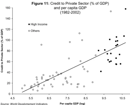
(21) In sum, higher volatility of terms of trade and quantities exported should not necessarily translate into higher aggregate volatility. If residents can access international capital markets, they will hold a well-diversified portfolio that is suitable to smoothing cash flow fluctuations associated with fluctuations in trade revenues. Even if market imperfections exist, fluctuations can still be buffered if suitable monetary policy instruments are available. This implies that a given amount of volatility in the terms of trade or external trade will have different effects on aggregate volatility, depending on the country’s financial development and the quality of the domestic financial institutions. In the following section we will use an interaction variable that combines the terms of trade volatility with financial development in order to test for the importance of this interaction in generating excess volatility. We will now examine other indicators that can help us to identify the effects on aggregate volatility of international credit market failures. 3. Contracts As was mentioned above, volatility and institutional weaknesses place severe constraints on the agents’ ability to implement some transactions that are mutually beneficial to them. The existence of these non-contractible transactions has very specific consequences on the financial side of the economy. It translates into missing financial markets, financial contracts of short duration, and dollarization. This, in turn, affects the operation of the shock-transmission mechanisms and makes the process of macroeconomic adjustment more volatile. The case studies will examine this in specific country contexts. In these notes we would like to highlight two observational consequences –referring to the financial system and macro adjustment– that are suitable to international comparison and will be useful as background to assess the findings of the case studies. If the environment is more volatile and institutions tend to be weaker in less developed countries, there should be a positive association between financial deepening and per capita GDP. Figure 11 shows the relationship between per capita GDP and the private credit/GDP ratio corresponding to the countries in our sample. As can be seen, there is a positive association between these two variables. This is not surprising because this fact has been very well documented and established in the literature, see Levine (1997).. 20.

(22) Figure 11: Credit to Private Sector (% of GDP) and per capita GDP (1982-2002). 160 140. Credit to Private Sector (% of GDP). High Income 120. Others. 100. 80 60. 40 20. 0 4.5. 5.5. 6.5. Source: World Develompment Indicators.. 7.5. 8.5. 9.5. 10.5. Per capita GDP (log). The second piece of evidence has to do with macroeconomic adjustment6. In those economies in which the duration of real and financial contracts is short, reduced inertia should be built into the system and, consequently, cyclical disturbances should fade away faster. Hence, given our assumptions about the contract structure in developing countries, it seems natural to expect the speed of macroeconomic adjustment to be higher when the the per capita GDP is lower. Of course, the counterpart of this faster adjustment speed would be excess volatility and elevated welfare costs of macroeconomic fluctuations. One natural way to test this hypothesis is to examine whether a relationship exists between the persistence of the cycle and per capita GDP. We will use the “velocity” at which GDP deviations reverse to the mean over the cycle as our cyclepersistence indicator. More specifically, we have used a univariate VAR to model each country’s cyclical disturbances and, then, have identified the speed of the adjustment with the proportion of the total response to the shock that takes place during the first three periods. The higher this proportion is, the higher the speed of adjustment and the lower the degree of persistence will be. Of course, for this indicator to be meaningful, we need high-frequency data. Hence, we will use an alternative sample based on quarterly data. Regrettably, the number of countries in the sample will be smaller because there are no quarterly data available for some of the countries under analysis. Figure 12 exhibits the results of the test for the countries in the sample, organized by per capita GDP in increasing order. The evidence is consistent with our hypothesis: The speed of adjustment tends to be higher in developing countries. Note, additionally, that the organization of the regions based on the regional mean speed of adjustment is consistent with our previous findings on volatility: The Latin American cycle is less persistent than the Asian one and the Euro Area shows the highest degree of cycle persistence. For example, on average, 65% of the total response to shocks in Latin American countries occurs during the first three periods, while the economies in. 6. In this part we rely on CEDES’ work on Macroeconomic Policy Coordination.. 21.

(23) the Euro Area and OECD complete only around 45% of the response in an equal number of periods. Figure 12: Persistency in GDP Cycle (1980-2004) by GDP per capita in 1995 US$ 1 0.9 0.8. Averages. 0.7 0.6 0.5 0.4 0.3 0.2 0.1. OECD. Denmark. Latin America. Norway. Germany. Austria. France. Canada. Italy. United Kingdom. Hong Kong. Portugal. Uruguay. Russia. South Africa. Chile. Malasya. Source: IMF.. Venezuela. Indonesia. 0. Period 3. 22.

(24) III. Detecting and Assessing Excess Volatility The complete-market approach has two straightforward predictions regarding the relationship between consumption and income volatility. First, private consumption volatility should be lower than income volatility to the extent that private agents use financial markets to smooth consumption. Second, the evolution of domestic consumption should be more correlated with the evolution of world consumption than with national income. We can use these two central predictions of the theoretical model to detect excess volatility costs. As we will see, neither of these two predictions holds and, consequently, we will argue that excess volatility is present in the countries of our sample. Although this is true for both developing and developed countries, the evidence clearly suggests that the problem of excess volatility is much worse in the case of developing economies. This raises the question of how far developing economies are from the excess volatility benchmark set by the countries where financial deepening is high. Note that this question seeks to identify that portion of excess volatility that can be attributed to a flawed financial structure –and thus to a weak DFA and imperfect links with the IFA– rather than to examine the effects of market failures on excess volatility in general. To tackle this latter question, we will model the behavior of consumption volatility using some of the volatility indicators that we have already examined as explanatory variables. We will then utilize the fitted consumption volatility equation to measure the size of excess volatility in economies where the functioning of institutions and the market mechanism is more imperfect. We will use the values predicted for the United States and Europe as our benchmark. That is, we will assume that these economies have achieved the lowest level of excess volatility that can be reached, given the constraints placed by transaction costs and other distortions. 1. Comparing Consumption and GDP volatility If the financial constraints that agents face in the countries under analysis were not strict, they would engage in consumption-smoothing and consumption volatility would be lower than income volatility. Under these circumstances, if we plotted consumption volatility against income volatility, the observations should all fall below the 45-degree line. As Figure 13 shows, this is not the case7.. 7. Note that we are using GDP and not national income. To the extent that national income is less volatile than GDP and there is some degree of international risk diversification, our test can be considered very exigent and biased in favor of accepting the null hypothesis that consumption is less volatile than income.. 23.

(25) Figure 13: Consumption Volatility and GDP Volatility (1960-2002). 0.16. 0.14. Consumption Volatility. 0.12. 0.1. 0.08. 0.06. 0.04. High Income Countries. 0.02. Others. 0 0. 0.02. 0.04. 0.06. 0.08. 0.1. 0.12. 0.14. 0.16. GDP Volatility. Source: World Develompment Indicators.. A large number of observations are situated well above the identity line. Note that there is a cluster of points situated on or below the line on the left side. The overwhelming majority of the observations pertaining to this cluster correspond to lowvolatility high-income countries (black points). A priori, this evidence suggests that financial constraints are softer and the quality of financial markets better in high-income regions, which is consistent with the close association between GDP per capita and financial deepening on which we have already commented. This is also consistent with the evidence in Tables 1 and 3. These tables show that mean consumption volatility is higher than income volatility in the case of developing countries while the opposite occurs in the Euro Area. The volatilities are equal in the case of the OECD countries. Note that no important differences exist under different international architectures. The following figure shows the GDP and consumption volatility by region during the globalization period. Figure 14a: GDP and Consumption Volatilty OECD Countries. (1990-2002). 0.2 0.18 0.16. GDP Vol (1990-2002). 0.14. Cons. Vol. (1990-2002). 0.12 0.1 0.08 0.06 0.04 0.02. United States. Switzerland. Spain. Sweden. Norway. Portugal. New Zeland. Mexico. Netherlands. Korea. Luxembourg. Italy. Japan. Ireland. Iceland. United Kingdom. Source: World Develompment Indicators.. Greece. France. Germany. Finland. Canada. Denmark. Austria. Belgium. Australia. 0. 24.

(26) Figure 14b: GDP and Consumption Volatilty Euro Area. (1990-2002). 0.2 0.18. GDP Vol (1990-2002). 0.16. Cons. Vol. (1990-2002). 0.14 0.12 0.1 0.08 0.06 0.04 0.02. Spain. Portugal. Netherlands. Luxembourg. Italy. Ireland. Greece. Germany. France. Finland. Belgium. Austria. 0. Source: World Develompment Indicators.. Figure 14c: GDP and Consumption Volatilty Latin American Countries. (1990-2002). 0.2 0.18. GDP Vol (1990-2002). 0.16. Cons. Vol. (1990-2002). 0.14 0.12 0.1 0.08 0.06 0.04 0.02. Mexico. Uruguay. Trinidad and T.. Peru. Paraguay. Nicaragua. Honduras. Guatemala. El Salvador. Ecuador. Dominican R.. Costa Rica. Colombia. Chile. Argentina. Brazil. 0. Source: World Develompment Indicators.. Figure 14d: GDP and Consumption Volatilty African Countries. (1990-2002). 0.2 0.18. GDP Vol (1990-2002). 0.16. Cons. Vol. (1990-2002). 0.14 0.12 0.1 0.08 0.06 0.04 0.02. Zambia. Zimbabwe. Tunisia. Togo. Senegal. South Africa. Nigeria. Rwanda. Morocco. Mauritania. Malawi. Madagascar. Kenya. Leshoto. Ghana. Gambia. Gabon. Cote D'Iv.. Egypt, A. R.. Congo. Cameroon. Burundi. Burkina F.. Benin. Algeria. 0. Source: World Develompment Indicators.. 25.

(27) Figure 14e: GDP and Consumption Volatilty Asian Countries. (1990-2002). 0.2 0.18. GDP Vol (1990-2002). 0.16. Cons. Vol. (1990-2002). 0.14 0.12 0.1 0.08 0.06 0.04 0.02. Korea. Japan. Thailand. Singapore. Phillipines. Pakistan. Malaysia. Indonesia. India. Hong Kong. Bangladesh. China. 0. Source: World Develompment Indicators.. Figure 14f: GDP and Consumption Volatilty Transition Countries. (1990-2002). 0.2 0.18. GDP Vol (1990-2002). 0.16. Cons. Vol. (1990-2002). 0.14 0.12 0.1 0.08 0.06 0.04 0.02 Ukraine. Slovak Republic. Russian Federation. Source: World Develompment Indicators.. Romania. Poland. Hungary. Czech Republic. Bulgaria. 0. If the residents of the countries in our sample had relatively fluent access to international capital markets, they would use them to diversify idiosyncratic risk away. Under these conditions, the evolution of domestic and world consumption should be correlated while there should not be a significant relationship between the growth rate of domestic consumption and GDP growth. To assess this prediction, we run regressions for each country with consumption growth as a dependent variable and world consumption growth8 and the country’s GDP growth as explanatory variables. If there are no external financial constraints, the coefficient corresponding to the first variable should be positive and significant and the second one should not be significant. The results are basically the opposite, as we can see in the following table.. 8. We have used OECD’s consumption as proxy.. 26.

(28) Table 5 Country Argentina Brazil Canada Chile Colombia Costa Rica Dominican Republic Ecuador Guatemala Honduras Mexico Nicaragua Paraguay Perú Trinidad y Tobago United States Uruguay Austria Belgium Denmark Finland France Germany Greece Iceland Ireland Italy Luxemburgo Netherlands Norway Portugal Spain Sweden Switzerland United Kingdom Algeria Benin Burkina Faso Burundi Cameroon Congo Cote D'Ivory Egypt, Arab. Rep. Gabon Gambia Ghana Kenya Leshoto Madagascar Malawi Mauritania Morocco Nigeria Rwanda Senegal South Africa Togo Tunisia Zambia Zimbabwe Bangladesh China Hong Kong India Indonesia Japan Korea Malasya Pakistan Phillipines Thailand Australia New Zeland Russia Bulgaria Czech Republic Hungary Poland Romania Slovak Republic Ukraine. Constant 0.007724 0.024372 0.002557 -0.057041 -0.004688 -0.004534 -0.006431 0.013188 0.001541 0.000184 -0.002044 -0.008651 0.023761 -0.018608 -0.000502 0.002945 -0.007558 0.009378 0.001816 -0.002316 -0.006065 -0.002623 0.001935 0.006499 -0.006925 -0.021279 0.003212 0.014066 -0.004706 -0.002423 0.014490 -0.003934 -0.005193 -0.003108 0.009820 0.039752 -0.013034 0.009670 0.012763 0.006433 -0.019432 -0.021226 0.018300 -0.063621 -0.042603 -0.019273 0.021181 -0.010027 -0.008116 0.008224 0.083009 0.005506 0.056247 0.004347 0.001370 0.002824 -0.000173 0.023148 -0.036611 -0.018095 0.015278 0.035691 0.006066 0.002615 0.073325 -0.001389 0.000073 -0.000114 0.000591 0.010316 -0.002349 0.010389 -0.006100 0.049607 -0.027259 -0.001540 0.017203 0.047619 0.006763 -0.032361 -0.111460. *. *. * *. *. *. *. *. *. * *. *. OECD's Consumption Growth Country's GDP Growth (*) the coefficient is significant at the 5% level. -0.239545 1,009788 -0.645325 0.835448 0.086716 0.737709 1,405219 1,756993 0.157084 0.919574 -0.014073 1,072449 0.353437 1,017734 -0.361435 0.697357 0.029016 0.715351 0.037612 0.695541 -0.020997 0.990364 0.241631 0.611387 -0.570941 0.878538 0.980672 * 0.903829 -0.298570 1,476861 0.317732 * 0.558125 0.126658 1,274383 0.046211 0.625637 0.493943 * 0.341567 -0.017452 0.909463 0.330019 * 0.860171 0.461280 * 0.538149 0.404397 0.475572 0.533908 0.395267 -0.143908 1,402522 0.750021 * 0.737442 0.170243 0.844950 0.347981 0.147325 0.312564 0.904390 0.129790 0.797238 -0.647427 0.996369 0.170352 0.935941 0.237536 0.691009 0.458112 * 0.426572 -0.200583 0.967835 -1,490345 1,292655 0.532582 1,138666 -0.493476 0.932597 -0.546866 0.969524 -0.390475 1,012049 -0.184041 0.889205 0.602237 0.921448 -0.036451 0.374089 3,227640 * -0.058846 1,568469 0.026585 0.286604 1,171222 -1,163950 1,198033 0.716057 0.395131 0.093216 0.814136 -0.608880 1,303466 -2,562778 * 0.945861 -0.176826 0.962123 -2,459346 * 0.600649 -0.126428 0.393974 -0.189385 0.603390 0.167593 0.544545 0.109306 0.600960 -0.284064 0.481312 0.713309 0.363857 0.907772 0.672208 -0.675762 0.780882 -0.532252 0.489472 0.345977 0.696571 -0.095653 0.685625 -2,016337 * 0.609037 0.497202 * 0.620240 -0.161704 0.931707 -0.568876 1,109572 -0.670618 1,361476 -0.061220 0.364230 -0.083071 0.877938 0.083577 0.377623 0.328452 0.609841 -1,680829 0.430341 1,379839 0.767310 0.344986 1,649865 -0.616208 0.713477 -0.355998 0.066568 0.524526 1,116785 1,233314 1,424102 6,125018 0.672453. * * * * * * * * * * * * * * * * * * * * * * * * * * * * * * * * * * * * * * * * * *. * * * * * * * * * * * *. * * * * * * * * * * * * * * * * * * *. 27.

(29) 2. Identifying Shocks and Excess Volatility If markets functioned efficiently, agents would only bear an optimal amount of “fundamental” risk in equilibrium. When financial market failures are the norm rather than the exception, agents will bear excess risk. Hence, suppose that markets were functioning reasonably well and we wanted to estimate an equation explaining consumption volatility. If we introduced an indicator of financial deepening as an explanatory variable into the equation explaining consumption volatility, the coefficient of such a variable would not be significantly different from zero. Based on this rationale, our strategy to test for the presence of and to measure excess volatility consists of two steps. First, we will introduce different proxies for market failures into a consumption volatility equation. If the coefficient corresponding to this variable is statistically relevant, we will interpret this to indicate that excess volatility originating in financial market failures is present in the countries of our sample. Second, we will use the value of the estimated coefficient to measure the size of excess volatility present in specific countries of our sample. As we have already mentioned, developing countries’ excess volatility level will be benchmarked against developed-country levels rather than against the level predicted by the theoretical model. More specifically, the level of country x’s excess volatility will be calculated as the difference between the level of consumption volatility predicted by our equation for country x and the level of consumption volatility that would have been observed if country x had had the level of financial deepening achieved by the benchmark country9. We identify this latter level with the portion of volatility resulting from "fundamental10" sources. We will use an interaction variable as our indicator of market failures: the volatility of the terms of trade divided by the level of domestic financial deepening achieved by the country. The idea is simple: The volatility of the terms of trade should not be relevant to explaining consumption volatility if financial markets can be used to diversify risk away. Hence, if financial market failures are important, we would expect that the higher the volatility of the terms of trade and the lower financial deepening are, the higher the volatility of consumption is. The consumption volatility equation will be estimated on the basis of data corresponding to the globalization period (1990-2002). To identify the effects of financial market failures on consumption growth volatility, we need to control for other shocks affecting aggregate consumption volatility, which generate "fundamental" volatility. We will use per capita GDP and the volatility of the output growth rate as controls11. Given that this volatility variable can be simultaneously determined together 9. This implies replacing the value of the financial deepening indicator corresponding to country x by the value corresponding to the benchmark country in the fitted equation. 10 In the context of this discussion of estimation results, we use the word "fundamental" descriptively to stress the role of financial market failures. It does not reflect the theoretical concept; note that GDP volatility, for example, will reflect other market failures, such as imperfect competition in labor markets and so on. 11 The effects of different sources of shocks are very difficult to identify. We elaborated on this in the background paper. Wolf (2004), for example, classifies shocks in three categories: (1) exogenous shocks, which are outside the control of households and policy makers (commodity price influencing terms of trade; world interest rates, climate, natural disaster); (2) endogenous shocks (unstable macro policies,. 28.

(30) with consumption volatility, we will use the volatility of GDP in the previous decade (1980-1989) as an instrument to account for the probable presence of a simultaneity bias. Since this is a counterfactual exercise, we would like to stress that its primary objective is heuristic. We would also like to call attention to the fact that data availability places serious constraints on the quality of the estimation. In particular, multicollinearity problems are significant. This is why we will present alternative versions of the consumption volatility equation using alternative indicators of financial failures and alternative controls for other sources of shocks. We have also checked for endogeneity bias by utilizing instruments when possible. Table 6 Dependent Variable: Consumption growth volatility Method: Least Squares White Heteroskedasticity-Consistent Standard Errors & Covariance Included Observations: 73 R-squared: 0.55 Variable. Coefficient. "t" Value. Constant. 0.059029. 2.470012. GDP Growth Volatility (1980-1989). 0.766482. 3.096465. Per Capita GDP (1990-2002). -0.005639. -2.587927. Terms of Trade Volatility / Private Sector Credit / GDP (1990-2002). 1.711816. 2.427048. Fresh Money. As can be seen, all coefficients are significant at the 5% level and the signs are those expected based on our previous discussion of the analytical and empirical issues associated with volatility. According to the estimated equation, the lower the per capita GDP and the higher output volatility are, the higher consumption volatility will be. These are "fundamental" sources of volatility. Note, additionally, that the coefficient of the per capita GDP may reflect the influence of institutional factors to the extent that there is a close association between the income level and institutional development. Since the coefficient corresponding to the financial failure indicator is significant, we can conclude that excess volatility stemming from imperfections in capital markets is likely to be present. Figures 15a-f show the estimations of the amounts of excess volatility that are present in each country. These results suggest an ordering among regions that is consistent with our previous findings: The Euro area is the region with the lowest level of excess volatility. Among developing countries, African economies show the highest level of excess volatility, followed by Latin America, Transition countries, and Asia. Indeed, in terms of the research project, we explain the presence of this kind of excess consumption volatility as the result of the institutional weaknesses in the DFA and the linkages with the IFA.. political instability, financial crises brought about by domestic imperfections); and (3) mixed (endogenous/exogenous), which are associated with productivity shocks and capital flows. The compounded effects of these shocks reflect on GDP volatility.. 29.

(31) Figure 15a: Fundamental Volatility and Excess Volatility due to Financial Market Failures. OECD Countries. (1990-2002). 0.10. 0.08. Fundamental Volatility Excess Volatility. 0.06. 0.04. 0.02. Poland. Slovak Rep.. Hungary. Czech Rep.. New Zeland. Korea. Australia. Japan. Switzerland. Source: World Develompment Indicators.. United Kingdom. Spain. Sweden. Norway. Portugal. Netherlands. Italy. Luxembourg. Ireland. Iceland. Greece. France. Germany. Finland. Denmark. Austria. Belgium. Mexico. -0.02. United States. Canada. 0.00. Figure 15b: Fundamental Volatility and Excess Volatility due to Financial Market Failures. Euro Area. (1990-2002). 0.10. Fundamental Volatility 0.08. Excess Volatility. 0.06. 0.04. 0.02. Spain. Portugal. Netherlands. -0.02. Luxembourg. Italy. Ireland. Greece. Germany. France. Finland. Belgium. Austria. 0.00. Source: World Develompment Indicators.. Figure 15c: Fundamental and Excess Volatility due to Financial Market Failures Latin American Countries. (1990-2002). 0.1 0.09 0.08 0.07 0.06 0.05 0.04 0.03 0.02 0.01. Source: World Develompment Indicators.. Fundamental Volatility. Uruguay. Trinidad and T.. Peru. Paraguay. Nicaragua. Mexico. Honduras. Guatemala. Ecuador. Dom. R.. Costa Rica. Colombia. Chile. Brazil. Argentina. 0. Excess Volatility. 30.

(32) Figure 15d: Fundamental Volatility and Excess Volatility due to Financial Market Failures. African Countries. (1990-2002). 0.1. 0.08. 0.06. 0.04. 0.02. Zambia. Zimbabwe. Togo. Tunisia. Senegal. Fundamental Volatility. Source: World Develompment Indicators.. South Africa. Nigeria. Rwanda. Morocco. Malawi. Mauritania. Madagascar. Kenya. Leshoto. Ghana. Gabon. Gambia. Egypt, Rep.. Congo. Cote D'Ivory. Burundi. Cameroon. Benin. -0.02. Burkina F.. Algeria. 0. Excess Volatility. Figure 15e: Fundamental Volatility and Excess Volatility due to Financial Market Failures. Asian Countries. (1990-2002). 0.10. Fundamental Volatility Excess Volatility. 0.08. 0.06. 0.04. 0.02. Thailand. Phillipines. Pakistan. Malaysia. Korea. Japan. India. Indonesia. China. Hong Kong. -0.02. Bangladesh. 0.00. Source: World Develompment Indicators.. Figure 15f: Fundamental Volatility and Excess Volatility due to Financial Market Failures. Transition Countries. (1990-2002). 0.1 0.09 0.08 0.07 0.06 0.05 0.04 0.03 0.02 0.01. Source: World Develompment Indicators.. Fundamental Volatility. Ukraine. Slovak Rep.. Romania. Poland. Hungary. Czech Rep.. Bulgaria. Russia. 0. Excess Volatility. 31.

(33) Given the difficulties to define a "good" indicator to capture the effects of financial market failures on volatility, we have tried other specifications. The main purpose is to assess the sensitivity of the results to the specification of the model and the definition of the proxies for market failures. We will comment on two additional specifications. The first tests for the influence of financial deepening and the volatility coming from external shocks on consumption volatility. The coefficients corresponding to the credit/GDP and to the volatility of the terms of trade should not be significant. In particular, if the coefficient of the terms of trade were significant, it would indicate a lack of diversification of the country's idiosyncratic risks. In this specification, we have to drop the per capita GDP because of multicollinearity problems (financial deepening and GDP are highly collinear). The results presented in Table 7 are consistent with the hypothesis that both low domestic financial deepening and imperfect management of national idiosyncratic risk contribute to generating excess consumption volatility. Table 7 Dependent Variable: Consumption growth volatility Method: Least Squares White Heteroskedasticity-Consistent Standard Errors & Covariance Included Observations: 73 R-squared: 0.50 Variable Constant. Coefficient. "t" Value. 0.012968. 1.106952. GDP Growth Volatility (1980-1989). 0.758819. 2.902733. Terms of Trade Volatility (1990-2002). 0.199176. 2.881798. Private Sector Credit / GDP Ratio (1990-2002). -0.000133. -1.698624. The last specification addresses the role of "fresh money". We have argued that the higher the size of capital inflows vis-à-vis the openness is, the higher aggregate volatility will be. Hence, we have replaced the financial deepening indicator in our equation with the fresh money/exports ratio. As can be seen in Table 8, the results are similar to those obtained when using the credit/GDP ratio. All coefficients are significant and have the correct sign. Table 8 Dependent Variable: Consumption growth volatility Method: Least Squares White Heteroskedasticity-Consistent Standard Errors & Covariance Included Observations: 66 R-squared: 0.66 Variable Constant. Coefficient. "t" Value. -0.016204. -2.727608. GDP Growth Volatility (1990-2002). 0.764365. 4.361837. Terms of Trade Volatility (1990-2002). 0.316658. 4.342803. Fresh Money (1990-2002). 0.133278. 2.769165. 32.

(34) 3. Final Comments The evidence on international aggregate volatility that we have presented and discussed suggests the following conclusions. First, the central hypotheses of the project that place institutional weaknesses, financial market failures, and excess volatility in developing countries at center stage are plausible and relevant. The evidence on consumption and output volatility indicates that significant regional differences in volatility exist and that there have been important changes over time. Likewise, the importance of the level of per capita GDP to explain consumption volatility may reflect the fact that institutional and economic development are closely related. Hence, the project’s approach to institution building that emphasizes the role of regional factors, as well as the changes in the multilateral financial architecture, seems pertinent. Second, the analysis of the volatility of output and consumption and its determinants in light of the predictions of the theoretical complete-market model can be a very potent instrument to detect excess volatility. In addition, evidence indicates that much more research is necessary on the complex causal connections between the volatility of domestic absorption and the volatility of capital flows, especially in the case of relatively closed economies. We have focused on consumption, but note that excess investment volatility costs could have strong deleterious effects on the potential growth rate of developing countries. Third, the stylized facts that we have identified suggest that idiosyncratic structural features and the specific interactions between them are relevant to explain aggregate volatility. The lack of financial deepening, low trade openness coupled with deficient and volatile access to international markets, and the volatility of the export proceeds seems to be particularly relevant. Fourth, although international comparisons are useful to provide a benchmark for the country studies, these notes also show the limited value of cross-country studies as a way to shed light on: (a) the sources of shocks and the concrete way in which transmission mechanisms operate to amplify or reduce the incidence of shocks; (b) the relationship between micro and macro determinants of risk –the lack of export diversification, terms of trade volatility, the lack of capital and insurance markets, and so on; (c) the institutional details that make the DFA and the links with the IFA inefficient. These limitations tell us that the analysis of these issues in the context of country studies makes sense and can undoubtedly contribute to our understanding of the interactions between aggregate volatility and institutions.. 33.

(35) References Caballero, Ricardo J. (2003), On the International Financial Architecture:Insuring Emerging Markets, NBER Working Paper 9570. Feldstein, M., and C. Horioka. (1980). Domestic Savings and International Capital Flows. Economic Journal 90 (June): 314-329. Levine R. (1997), "Financial Development and Economic Growth: Views and Agenda", Journal of Economic Literature, Vol.35. Obstfeld, Maurice. (2004), Globalization, Macroeconomic Performance, and The Exchange Rates of Emerging Economies. NBER. Working Paper 10849. World Bank (2004), World Development Indicators 2004.. 34.

(36)